Answers to Selected Problems

on apples gives him more extra utils than a dollar
spent on kumquats. Thus, Andy maximizes his utility
by spending all his money on apples and buying
40/2 = 20 pounds of apples.
4.14 David’s marginal utility of q 1 is 1 and his marginal util-
ity of q2 is 2. The slope of David’s indifference curve is
-U1 /U2 = - 1
2 . Because the marginal utility from one
extra unit of q2 = 2 is twice that from one extra unit
of q1 , if the price of q2 is less than twice that of q1 ,
David buys only q2 = Y/p2 , where Y is his income and
p2 is the price. If the price of q2 is more than twice that
of q1 , David buys only q1 . If the price of q2 is exactly
twice as much as that of q1 , he is indifferent between
buying any bundle along his budget line.
4.15 Vasco determines his optimal bundle by equating
the ratios of each good’s marginal utility to its price.
a. At the original prices, this condition is
U1 /10 = 2q1q2 = 2q2 1 = U2 /5. Thus, by dividing
both sides of the middle equality by 2q1 ,
we know that his optimal bundle has the property
that q1 = q2 . His budget constraint is
90 = 10q1 + 5q2 . Substituting q2 for q1 , we find
that 15q2 = 90, or q2 = 6 = q1 .
b. At the new price, the optimum condition
requires that U1 /10 = 2q1q2 = 2q2 1 = U2 /10, or
2q2 = q1 . By substituting this condition into his
budget constraint, 90 = 10q1 + 10q2 , and solving,
we learn that q2 = 3 and q1 = 6. Thus, as
the price of chickens doubles, he cuts his consumption
of chicken in half but does not change
how many slabs of ribs he eats.
6.2 Change the labels on the figure in the Challenge
Solution to illustrate the answer to this question:
When the price in Canada is relative low, the motorist
buys gasoline in Canada, and vice versa.
Chapter 4
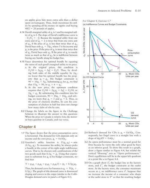
1.7 The figure shows that the price-consumption curve
is horizontal. The demand for CDs depends only on
income and the own price, q 1 = 0.6Y/p 1 .
2.2 Guerdon’s utility function is U(q 1 , q 2 ) = min
(0.5q 1 , q 2 ). To maximize his utility, he always picks
a bundle at the corner of his right-angle indifference
curves. That is, he chooses only combinations of the
two goods such that 0.5q 1 = q 2 . Using that expression
to substitute for q 2 in his budget constraint, we
find that
Y = p 1 q 1 + p 2 q 2 = p 1 q 1 + p 2 q 1 /2 = (p 1 + 0.5p 2 )q 1 .
Thus, his demand curve for bananas is q 1 = Y/(p 1 +
0.5p 2 ). The graph of this demand curve is downward
sloping and convex to the origin (similar to the Cobb-
Douglas demand curve in panel a of Figure 4.1).
Answers to Selected Problems
For Chapter 4, Exercise 1.7
(a) Indifference Curves and Budget Constraints
q 2 , Movie DVDs, Units per year
6
45
15
6
E-35
L
0
1
L2 L3 I 1
I 2
4 12
(b) CD Demand Curve
30 q1 , Music CDs,
Units per year
p 1 , $ per units
e 1
E 1
e 2
E 2
0 4 12 30
2.4 Barbara’s demand for CDs is q1 = 0.6Y/p1 . Consequently,
her Engel curve is a straight line with a
slope of dq1 /dY = 0.6/p1 .
3.2 An opera performance must be a normal good for
Don because he views the only other good he buys
as an inferior good. To show this result in a graph,
draw a figure similar to Figure 4.4, but relabel the
vertical “Housing” axis as “Opera performances.”
Don’s equilibrium will be in the upper-left quadrant
at a point like a in Figure 4.4.
3.5 On a graph show L f , the budget line at the factory
store, and L o , the budget constraint at the outlet
store. At the factory store, the consumer maximum
occurs at ef on indifference curve If . Suppose that
we increase the income of a consumer who shops
at the outlet store to Y* so that the resulting budget
e 3
E 3
Priceconsumption
curve
I 3
CD
demand
curve
q 1 , Music CDs,
Units per year