Answers to Selected Problems

dD(14.70 + τ)
-S(14.70 + τ)] - τ J -
dτ
dS(14.70 + τ)
dD(14.70 + τ)
= -τ J
dτ
- dS(14.70 + τ)
R.
dτ
R
dτ
If we evaluate this expression at τ = 0, we find that
dDWL/dτ = 0. In short, applying a small tariff to
the free-trade equilibrium has a negligible effect on
quantity and deadweight loss. Only if the tariff is
larger—as in Figure 9.9—do we see a measurable
effect.
Chapter 10
1.7 A subsidy is a negative tax. Thus, we can use the
same analysis that we used in Solved Problem 10.1
to answer this question by reversing the signs of the
effects.
4.1 If you draw the convex production possibility frontier
on Figure 10.5, you will see that it lies strictly
inside the concave production possibility frontier.
Thus, more output can be obtained if Jane and
Denise use the concave frontier. That is, each should
specialize in producing the good for which she has a
comparative advantage.
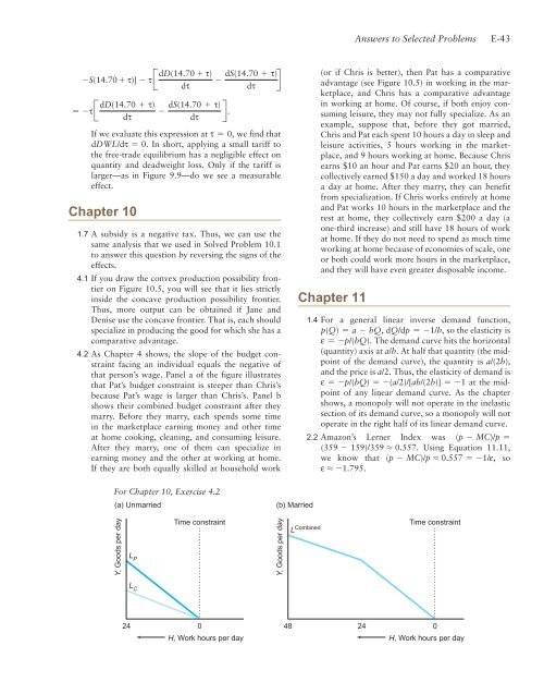
4.2 As Chapter 4 shows, the slope of the budget constraint
facing an individual equals the negative of
that person’s wage. Panel a of the figure illustrates
that Pat’s budget constraint is steeper than Chris’s
because Pat’s wage is larger than Chris’s. Panel b
shows their combined budget constraint after they
marry. Before they marry, each spends some time
in the marketplace earning money and other time
at home cooking, cleaning, and consuming leisure.
After they marry, one of them can specialize in
earning money and the other at working at home.
If they are both equally skilled at household work
For Chapter 10, Exercise 4.2
(a) Unmarried
Y, Goods per day
L P
L C
Time constraint
24 0
H, Work hours per day
(b) Married
Y, Goods per day
Answers to Selected Problems
E-43
(or if Chris is better), then Pat has a comparative
advantage (see Figure 10.5) in working in the marketplace,
and Chris has a comparative advantage
in working at home. Of course, if both enjoy consuming
leisure, they may not fully specialize. As an
example, suppose that, before they got married,
Chris and Pat each spent 10 hours a day in sleep and
leisure activities, 5 hours working in the marketplace,
and 9 hours working at home. Because Chris
earns $10 an hour and Pat earns $20 an hour, they
collectively earned $150 a day and worked 18 hours
a day at home. After they marry, they can benefit
from specialization. If Chris works entirely at home
and Pat works 10 hours in the marketplace and the
rest at home, they collectively earn $200 a day (a
one-third increase) and still have 18 hours of work
at home. If they do not need to spend as much time
working at home because of economies of scale, one
or both could work more hours in the marketplace,
and they will have even greater disposable income.
Chapter 11
1.4 For a general linear inverse demand function,
p(Q) = a - bQ, dQ/dp = -1/b, so the elasticity is
ε = -p/(bQ). The demand curve hits the horizontal
(quantity) axis at a/b. At half that quantity (the midpoint
of the demand curve), the quantity is a/(2b),
and the price is a/2. Thus, the elasticity of demand is
ε = -p/(bQ) = -(a/2)/[ab/(2b)] = -1 at the midpoint
of any linear demand curve. As the chapter
shows, a monopoly will not operate in the inelastic
section of its demand curve, so a monopoly will not
operate in the right half of its linear demand curve.
2.2 Amazon’s Lerner Index was (p - MC)/p =
(359 - 159)/359 L 0.557. Using Equation 11.11,
we know that (p - MC)/p L 0.557 = -1/ε, so
ε L -1.795.
L Combined
Time constraint
48 24
0
H, Work hours per day