Answers to Selected Problems

E-32
Answers to Selected
Problems
I know the answer! The answer lies within the heart of all mankind! The answer is twelve?
I think I’m in the wrong building. —Charles Schultz
Chapter 2
1.1 The demand curve for pork is Q = 171 - 20p +
20pb + 3pc + 2Y. As a result, 0Q/0Y = 2. A $100
increase in income causes the quantity demanded to
increase by 0.2 million kg per year.
1.2 To solve this problem, we first rewrite the inverse
demand functions as demand functions and then add
them together. The total demand function is Q =
Q1 + Q2 = (120 - p) + 160 - 1
2 p2 = 180 - 1.5p.
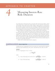
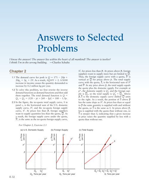
2.3 In the figure, the no-quota total supply curve, S in
panel c, is the horizontal sum of the U.S. domestic
supply curve, Sd , and the no-quota foreign supply
curve, S f . At prices less than p, foreign suppliers
want to supply quantities less than the quota, Q. As
a result, the foreign supply curve under the quota,
S f , is the same as the no-quota foreign supply curve,
For Chapter 2, Exercise 2.3
(a) U.S. Domestic Supply (b) Foreign Supply (c) Total Supply
p, Price
per ton
S d
p, Price
per ton
S f , for prices less than p. At prices above p, foreign
suppliers want to supply more but are limited to Q.
Thus, the foreign supply curve with a quota, Sf is
vertical at Q for prices above p. The total supply
curve with the quota, S, is the horizontal sum of Sd and Sf At any price above p, the total supply equals
the quota plus the domestic supply. For example at
p*, the domestic supply is Q * d and the foreign supply
is Qf , so the total supply is Q * d + Qf . Above
p, S is the domestic supply curve shifted Q units
to the right. As a result, the portion of S above p
has the same slope as Sd . At prices less than or equal
to p the same quantity is supplied with and without
the quota, so S is the same as S. At prices above p,
less is supplied with the quota than without one, so
S is steeper than S, indicating that a given increase
in price raises the quantity supplied by less with a
quota than without one.
p, Price
per ton
p* p* p*
p –
–
Qd Q *
d
–
Qf Q *
f
Qd , Tons per year Qf , Tons per year
p –
S f –
S f
p –
S –
S
– –
Qd + Qf –
Q * + Q d f Q * + Q *
d f
Q, Tons per year

3.1 The statement “Talk is cheap because supply exceeds
demand” makes sense if we interpret it to mean that
the quantity of talk supplied exceeds the quantity
demanded at a price of zero. Imagine a downwardsloping
demand curve that hits the horizontal, quantity
axis to the left of where the upward-sloping
supply curve hits the axis. (The correct aphorism is
“Talk is cheap until you hire a lawyer.”)
3.3 Equating the right-hand sides of the tomato supply
and demand functions and using algebra, we find
that ln p = 3.2 + 0.2 ln p t . We then set p t = 110,
solve for ln p, and exponentiate ln p to obtain the
equilibrium price, p L $62.80 per ton. Substituting
p into the supply curve and exponentiating, we
determine the equilibrium quantity, Q L 11.91 million
short tons per year.
4.3 To determine the equilibrium price, we equate the
right-hand sides of the supply function, Q = 20 +
3p - 20r, and the demand function, Q =
220 - 2p, to obtain 20 + 3p - 20r = 220 - 2p.
Using algebra, we can rewrite the equilibrium price
equation as p = 40 + 4r. Substituting this expression
into the demand function, we learn that the
equilibrium quantity is Q = 220 - 2(40 + 4r), or
Q = 140 - 8r. By differentiating our two equilibrium
conditions with respect to r, we obtain our comparative
statics results: dp/dr = 4 and dQ/dr = -8.
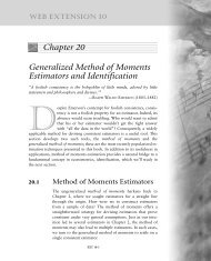
4.7 The graph reproduces the no-quota total American
supply curve of steel, S, and the total supply curve
under the quota, S, which we derived in the answer
to Exercise 2.3. At a price below p, the two supply
curves are identical because the quota is not binding:
It is greater than the quantity foreign firms want to
supply. Above p, S lies to the left of S. Suppose that
the American demand is relatively low at any given
price so that the demand curve, D l , intersects both
the supply curves at a price below p. The equilibria
For Chapter 2, Exercise 4.7
p, Price of steel per ton
p3 p2 p
p1 –
Q 1
e 1
e 3
D l (low)
e2
Q 3 Q 2
–
S (quota)
S (no quota)
D h (high)
Q,Tons of steel
per year
Answers to Selected Problems
E-33
both before and after the quota is imposed are at e1 ,
where the equilibrium price, p1 , is less than p. Thus,
if the demand curve lies near enough to the origin
that the quota is not binding, the quota has no effect
on the equilibrium. With a relatively high demand
curve, Dh , the quota affects the equilibrium. The
no-quota equilibrium is e2 , where Dh intersects the
no-quota total supply curve, S. After the quota is
imposed, the equilibrium is e3 , where Dh intersects
the total supply curve with the quota, S. The quota
raises the price of steel in the United States from p2 to p3 and reduces the quantity from Q2 to Q3 .
5.8 The elasticity of demand is (dQ/dp)(p/Q) = (-9.5
thousand metric tons per year per cent) * (45./1,275
thousand metric tons per year) L -0.34. That is,
for every 1% fall in the price, a third of a percent
more coconut oil is demanded. The cross-price
elasticity of demand for coconut oil with respect
to the price of palm oil is (dQ/dpp )(pp /Q) =
16.2 * (31/1,275) L 0.39.
6.4 We showed that, in a competitive market, the effect
of a specific tax is the same whether it is placed on
suppliers or demanders. Thus, if the market for milk
is competitive, consumers will pay the same price in
equilibrium regardless of whether the government
taxes consumers or stores.
6.8 Differentiating quantity, Q(p(τ)), with respect to
τ, we learn that the change in quantity as the tax
changes is (dQ/dp)(dp/dτ). Multiplying and dividing
this expression by p/Q, we find that the change
in quantity as the tax changes is ε(Q/p)(dp/dτ).
Thus, the closer ε is to zero, the less the quantity
falls, all else the same.
Because R = p(τ)Q(p(τ)), an increase in the tax
rate changes revenues by
dR
dτ
dR
dτ
dp dQ
= Q + p
dτ dp dp
dτ ,
using the chain rule. Using algebra, we can rewrite
this expression as
= dp
dτ
dQ dp dQ
¢Q + p ≤ = Q¢1 +
dp dτ
dp p dp
≤ = Q(1 + ε).
Q dτ
Thus, the effect of a change in τ on R depends on
the elasticity of demand, ε. Revenue rises with the
tax if demand is inelastic (-1 6 ε 6 0) and falls if
demand is elastic (ε 6 -1).
7.3 A usury law is a price ceiling, which causes the
quantity that firms want to supply to fall.
7.4 We can determine how the total wage payment,
W = wL(w), varies with respect to w by differentiating.
We then use algebra to express this result in
terms of an elasticity:
dW
dw
dL
dL
= L + w = L¢1 +
dw dw w
L
≤ = L(1 + ε),

E-34 Answers to Selected Problems
where ε is the elasticity of demand of labor. The sign
of dW/dw is the same as that of 1 + ε. Thus, total
labor payment decreases as the minimum wage forces
up the wage if labor demand is elastic, ε 6 -1, and
increases if labor demand is inelastic, ε 7 -1.
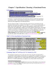
9.2 Shifts of both the U.S. supply and U.S. demand curves
affected the U.S. equilibrium. U.S. beef consumers’
fear of mad cow disease caused their demand curve
in the figure to shift slightly to the left from D1 to
D2 . In the short run, total U.S. production was essentially
unchanged. Because of the ban on exports, beef
that would have been sold in Japan and elsewhere
was sold in the United States, causing the U.S. supply
curve to shift to the right from S1 to S2 . As a
result, the U.S. equilibrium changed from e1 (where
S1 intersects D1 ) to e2 (where S2 intersects D2 ). The
U.S. price fell 15% from p1 to p2 = 0.85p1 , while
the quantity rose 43% from Q1 to Q2 = 1.43Q1 .
Comment: Depending on exactly how the U.S. supply
and demand curves had shifted, it would have been
possible for the U.S. price and quantity to have both
fallen. For example, if D2 had shifted far enough left,
it could have intersected S2 to the left of Q1 , and the
equilibrium quantity would have fallen.
For Chapter 2, Exercise 9.2
p, Price per pound
p 1
p 2 = 0.85p 1
Chapter 3
e 1
S 1
D 1
D 2
Q 1 Q 2 = 1.43Q 1
Q, Tons of beef per year
1.5 If the neutral product is on the vertical axis, the
indifference curves are parallel vertical lines.
2.2 Sofia’s indifference curves are right angles (as in panel b
of Figure 3.5). Her utility function is U = min(H, W),
where min means the minimum of the two arguments,
H is the number of units of hot dogs, and W is the
number of units of whipped cream.
2.4 If we apply the transformation function F(x) = x ρ
to the original utility function, we obtain the new
utility function V(q 1 , q 2 ) = F(U(q 1 , q 2 )) = [(q 1 ρ +
e 2
S 2
q 2 ρ ) 1/ρ ] ρ = q1 ρ + q2 ρ , which has the same preference
properties as does the original function.
2.5 Given the original utility function, U, the consumer’s
marginal rate of substitution is -U 1 /U 2 . If V(q 1 ,
q 2 ) = F(U(q 1 , q 2 )), the new marginal rate of substitution
is -V 1 /V 2 = -[(dF/dU)U 1 ]/[(dF/dU)U 2 ] =
-U 1 /U 2 , which is the same as originally.
2.6 By differentiating we know that
U1 = a(aqρ 1 + [1 - a]qρ 2 )(1 - ρ)/ρqρ - 1
1 and
U2 = [1 - a](aqρ 1 + [1 - a]qρ 2 )(1 - ρ)/ρqρ - 1
2 .
Thus, MRS = -U1 /U2 = -[(1 - a)/a](q1 /q2 ) ρ - 1 .
3.1 Suppose that Dale purchases two goods at prices
p 1 and p 2 . If her original income is Y, the intercept
of the budget line on the Good 1 axis (where the
consumer buys only Good 1) is Y/p 1 . Similarly, the
intercept is Y/p 2 on the Good 2 axis. A 50% income
tax lowers income to half its original level, Y/2. As a
result, the budget line shifts inward toward the origin.
The intercepts on the Good 1 and Good 2 axes
are Y/(2p 1 ) and Y/(2p 2 ), respectively. The opportunity
set shrinks by the area between the original
budget line and the new line.
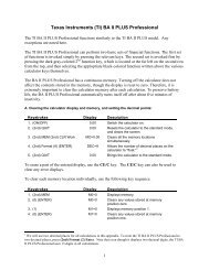
3.3 In the figure, the consumer can afford to buy up to
12 thousand gallons of water a week if not constrained.
The opportunity set, area A and B, is
bounded by the axes and the budget line. A vertical
line at 10 thousand on the water axis indicates the
quota. The new opportunity set, area A, is bounded
by the axes, the budget line, and the quota line.
Because of the rationing, the consumer loses part
of the original opportunity set: the triangle B to the
right of the 10-thousand-gallons quota line. The consumer
has fewer opportunities because of rationing.
For Chapter 3, Exercise 3.3
Other goods per week
Budget line
Quota
A B
0 10 12
Water, thousand gallons per month
4.3 Andy’s marginal utility of apples divided by the
price of apples is 3/2 = 1.5. The marginal utility
for kumquats is 5/4 = 1.2. That is, a dollar spent

on apples gives him more extra utils than a dollar
spent on kumquats. Thus, Andy maximizes his utility
by spending all his money on apples and buying
40/2 = 20 pounds of apples.
4.14 David’s marginal utility of q 1 is 1 and his marginal util-
ity of q2 is 2. The slope of David’s indifference curve is
-U1 /U2 = - 1
2 . Because the marginal utility from one
extra unit of q2 = 2 is twice that from one extra unit
of q1 , if the price of q2 is less than twice that of q1 ,
David buys only q2 = Y/p2 , where Y is his income and
p2 is the price. If the price of q2 is more than twice that
of q1 , David buys only q1 . If the price of q2 is exactly
twice as much as that of q1 , he is indifferent between
buying any bundle along his budget line.
4.15 Vasco determines his optimal bundle by equating
the ratios of each good’s marginal utility to its price.
a. At the original prices, this condition is
U1 /10 = 2q1q2 = 2q2 1 = U2 /5. Thus, by dividing
both sides of the middle equality by 2q1 ,
we know that his optimal bundle has the property
that q1 = q2 . His budget constraint is
90 = 10q1 + 5q2 . Substituting q2 for q1 , we find
that 15q2 = 90, or q2 = 6 = q1 .
b. At the new price, the optimum condition
requires that U1 /10 = 2q1q2 = 2q2 1 = U2 /10, or
2q2 = q1 . By substituting this condition into his
budget constraint, 90 = 10q1 + 10q2 , and solving,
we learn that q2 = 3 and q1 = 6. Thus, as
the price of chickens doubles, he cuts his consumption
of chicken in half but does not change
how many slabs of ribs he eats.
6.2 Change the labels on the figure in the Challenge
Solution to illustrate the answer to this question:
When the price in Canada is relative low, the motorist
buys gasoline in Canada, and vice versa.
Chapter 4
1.7 The figure shows that the price-consumption curve
is horizontal. The demand for CDs depends only on
income and the own price, q 1 = 0.6Y/p 1 .
2.2 Guerdon’s utility function is U(q 1 , q 2 ) = min
(0.5q 1 , q 2 ). To maximize his utility, he always picks
a bundle at the corner of his right-angle indifference
curves. That is, he chooses only combinations of the
two goods such that 0.5q 1 = q 2 . Using that expression
to substitute for q 2 in his budget constraint, we
find that
Y = p 1 q 1 + p 2 q 2 = p 1 q 1 + p 2 q 1 /2 = (p 1 + 0.5p 2 )q 1 .
Thus, his demand curve for bananas is q 1 = Y/(p 1 +
0.5p 2 ). The graph of this demand curve is downward
sloping and convex to the origin (similar to the Cobb-
Douglas demand curve in panel a of Figure 4.1).
Answers to Selected Problems
For Chapter 4, Exercise 1.7
(a) Indifference Curves and Budget Constraints
q 2 , Movie DVDs, Units per year
6
45
15
6
E-35
L
0
1
L2 L3 I 1
I 2
4 12
(b) CD Demand Curve
30 q1 , Music CDs,
Units per year
p 1 , $ per units
e 1
E 1
e 2
E 2
0 4 12 30
2.4 Barbara’s demand for CDs is q1 = 0.6Y/p1 . Consequently,
her Engel curve is a straight line with a
slope of dq1 /dY = 0.6/p1 .
3.2 An opera performance must be a normal good for
Don because he views the only other good he buys
as an inferior good. To show this result in a graph,
draw a figure similar to Figure 4.4, but relabel the
vertical “Housing” axis as “Opera performances.”
Don’s equilibrium will be in the upper-left quadrant
at a point like a in Figure 4.4.
3.5 On a graph show L f , the budget line at the factory
store, and L o , the budget constraint at the outlet
store. At the factory store, the consumer maximum
occurs at ef on indifference curve If . Suppose that
we increase the income of a consumer who shops
at the outlet store to Y* so that the resulting budget
e 3
E 3
Priceconsumption
curve
I 3
CD
demand
curve
q 1 , Music CDs,
Units per year

E-36 Answers to Selected Problems
line L* is tangent to the indifference curve If . The
consumer would buy Bundle e*. That is, the pure
substitution effect (the movement from ef to e*)
causes the consumer to buy relatively more firsts.
The total effect (the movement from ef to eo ) reflects
both the substitution effect (firsts are now relatively
less expensive) and the income effect (the consumer
is worse off after paying for shipping). The
income effect is small if (as seems reasonable) the
budget share of plates is small. An ad valorem tax
has qualitatively the same effect as a specific tax
because both taxes raise the relative price of firsts to
seconds.
3.7 We can determine the optimal bundle, e1 , at the
original prices p1 = p2 = 1 by using the demand
equation from Table 4.1: q1 = 4(p2 /p1 ) 2 = 4 and
q2 = Y/p2 - 4(p2 /p1 ) = 10 - 4 = 6. This optimal
bundle is on an indifference curve where
U = 4(4) 0.5 + 6 = 14.
At the new bundle, e2 , where p1 = 2 and p2 = 1,
q1 = 4(1/2) 2 = 1, and q2 = 10 - 4(1) = 8. This
optimal bundle is on an indifference curve where
U = 4(1) 0.5 + 8 = 12.
To determine e*, we want to stay on the original
indifference curve. We know that the tangency
condition will give the same q1 as at e2 because q1 depends on only the relative prices, so q1 = 1. The
question is what Y will compensate Phillip for the
higher price so that he can stay on the original indifference
curve. Because q2 = Y - 4(1/2) = Y - 4,
the utility is U = 1 + (Y - 4) = Y - 3. So the Y
that results in U = 14 is Y = 17. Thus, the substitution
effect is -3 (based on the movement from
e1 to e*) and the income effect is 0 (the movement
from e* to e2 ), so the total effect is -3 (movement
from e1 to e2 ).
3.9 At Sylvia’s optimal bundle, q1 = jq2 (see Chapter 3).
Otherwise, she could reduce her expenditure on
one of the goods and attain the same level of utility.
Because at the optimal bundle U = min(q1 , jq2 ), the
Hicksian demands are q1 = H1 (p1 , p2 , U) = U and
q2 = H2 (p1 , p2 , U) = U/j. The expenditure function
is E = p1q1 + p2q2 = p1U + p2U/j = (p1 + p2 /j)U.
4.1 The CPI accurately reflects the true cost of living
because Alix does not substitute between the goods
as the relative prices change.
Chapter 5
1.1 At a price of 30, the quantity demanded is 30, so the
consumer surplus is 1
2 (30 * 30) = 450, because the
demand curve is linear.
1.4 Hong and Wolak (2008) estimate that Area A is
$215 million and area B is $118 (= 333 - 215)
million (as you should have shown in your figure in
the answer to Exercise 1.3).
a. Given that the demand function is Q = Xp -1.6 ,
the revenue function is R(p) = pQ = Xp -0.6 .
Thus, the change in revenue, -$215 million,
equals R(39) - R(37) = X(39) -0.6 - X(37) -0.6 L
-0.00356X. Solving -0.00356X = -215, we
find that X L 60,353.
b. We follow the process in Solved Problem 5.1
39
60,353p-1.6dp1 = 60,353
0.6 p-0.6 2 39
∆CS = -
L37
37
L 100,588(39-0.6 - 37-0.6 )
L 100,588 * (-0.00356) L -358.
This total consumer surplus loss is larger than
the one estimated by Hong and Wolak (2008)
because they used a different demand function.
Given this total consumer surplus loss, area B is
$146 (= 358 - 215) million.
2.2 Because the good is inferior, the compensated demand
curves cut the uncompensated demand curve, D,
from below as the figure shows. Consequently,
CV = A, ∆CS = A + B, EV = A + B + C.
CV 6 ∆CS 6 EV .
For Chapter 5, Exercise 2.2
p, $ per unit
p 2
p 1
A
e 2
B
e 1
C
D
H EV
H CV
q 1 , Units per quarter
3.4 The two demand curves cross at e 1 in the diagram.
The price elasticity of demand, ε = (dQ/dp)(p/Q),
equals 1 over the slope of the demand curve, dp/dQ,
times the ratio of the price to the quantity. Thus, at e 1
where both demand curves have the same price, p 1 ,
and the same quantity, Q 1 , the steeper the demand
curve, the lower the elasticity of demand. If the
price rises from p 1 to p 2 , the consumer surplus falls
from A + C to A with the relatively elastic demand
curve (a loss of C) and from A + B + C + D to
A + B (a loss of C + D) with the relatively inelastic
demand curve.

For Chapter 5, Exercise 3.4
p, $ per unit
p 2
p 1
A
C
Relatively inelastic
demand (at e 1 )
B
e 3 D
Q 3
e 2
Q 2
Q, Units per week
5.8 The proposed tax system exempts an individual’s
first $10,000 of income. Suppose that a flat 10%
rate is charged on the remaining income. Someone
who earns $20,000 has an average tax rate of 5%,
whereas someone who earns $40,000 has an average
tax rate of 7.5%, so this tax system is progressive.
5.10 As the marginal tax rate on income increases, people
substitute away from work due to the pure substitution
effect. However, the income effect can be
either positive or negative, so the net effect of a tax
increase is ambiguous. Also, because wage rates differ
across countries, the initial level of income differs,
again adding to the theoretical ambiguity. If
we know that people work less as the marginal
tax rate increases, we can infer that the substitution
effect and the income effect go in the same
direction or that the substitution effect is larger.
However, Prescott’s (2004) evidence alone about
hours worked and marginal tax rates does not
allow us to draw such an inference because U.S. and
European workers may have different tastes and face
different wages.
5.11 The figure shows Julia’s original consumer equilibrium:
Originally, Julia’s budget constraint was a
straight line, L1 with a slope of -w, which was tangent
to her indifference curve I1 at e1 , so she worked
12 hours a day and consumed Y1 = 12w goods. The
maximum-hours restriction creates a kink in Julia’s
new budget constraint, L2 . This constraint is the
same as L1 up to eight hours of work, and is horizontal
at Y = 8w for more hours of work. The highest
indifference curve that touches this constraint is I2 .
Because of the restriction on the hours she can work,
e 1
Q 1
Relatively elastic
demand (at e 1 )
Answers to Selected Problems
E-37
Julia chooses to work eight hours a day and to consume
Y 2 = 8w goods, at e 2 . (She will not choose to
work fewer than eight hours. For her to do so, her
indifference curve I 2 would have to be tangent to the
downward-sloping section of the new budget constraint.
However, such an indifference curve would
have to cross the original indifference curve, I 1 , which
is impossible: see Chapter 3.) Thus, forcing Julia to
restrict her hours lowers her utility: I 2 must be below
I 1 .Comment: When I was in college, I was offered
a summer job in California. My employer said,
“You’re lucky you’re a male.” He claimed that, to
protect women (and children) from overwork, an
archaic law required him to pay women, but not
men, double overtime after eight hours of work. As
a result, he offered overtime work only to his male
employees. Such clearly discriminatory rules and
behavior are now prohibited. Today, however, both
females and males must be paid higher overtime
wages—typically 1.5 times as much as the usual
wage. Consequently, many employers do not let
employees work overtime.
For Chapter 5, Problem 5.11
Y, Goods per day
Y1 = 12w
Y 2 = 8w
L 1
L2
e 1
Time
constraint
I 1
I 2
24 H1 = 12 H2 = 8 H, Work hours
per day
6.2 Parents who do not receive subsidies prefer that
poor parents receive lump-sum payments rather
than a subsidized hourly rate for child care. If the
supply curve for child-care services is upward sloping,
by shifting the demand curve farther to the
right, the price subsidy raises the price of child-care
for these other parents.
6.3 The government could give a smaller lump-sum subsidy
that shifts the L LS curve down so that it is parallel
to the original curve but tangent to indifference
curve I 2 . This tangency point is to the left of e 2 , so
the parents would use fewer hours of child care than
with the original lump-sum payment.
e 2

E-38 Answers to Selected Problems
Chapter 6
3.1 One worker produces one unit of output, two workers
produce two units of output, and n workers produce
n units of output. Thus, the total product of
labor equals the number of workers: q = L. The
total product of labor curve is a straight line with a
slope of 1. Because we are told that each extra worker
produces one more unit of output, we know that the
marginal product of labor, dq/dL, is 1. By dividing
both sides of the production function, q = L, by L,
we find that the average product of labor, q/L, is 1.
3.4 (a) Given that the production function is
q = L 0.75 K 0.25 , the average product of labor, holding
capital fixed at K, is AP L = q/L = L -0.25 K 0.25 =
(K/L) 0.25 . (b) The marginal product of labor
is MP L = dq/dL = 3
4 (K/L)0.25 . (c) At K = 16,
AP L = 2L 0.25 and MP L = 1.5L 0.25 .
4.4 The isoquant looks like the “right angle” ones in
panel b of Figure 6.3 because the firm cannot substitute
between discs and machines but must use
them in equal proportions: one disc and one hour of
machine services.
4.8 Using Equation 6.8, we know that the marginal
rate of technical substitution is MRTS =
-MPL /MPK = - 2
3 .
4.9 The isoquant for q = 10 is a straight line that hits
the B axis at 10 and the G axis at 20. The marginal
product of B is MPB = 0q/ 0B = 1 everywhere
along the isoquant. Similarly, MPG = 0.5. Given that
B is on the horizontal axis, MRTS = -MPB /MPG = -1/0.5 = -2.
5.4 This production function is a Cobb-Douglas production
function. Even though it has three inputs
instead of two, the same logic applies. Thus, we can
calculate the returns to scale as the sum of the exponents:
γ = 0.27 + 0.16 + 0.61 = 1.04. That is, it
has (nearly) constant returns to scale. The marginal
product of material is
0q/0M = 0.61L 0.27 K 0.16 M -0.39 = 0.61q/M.
6.4 The marginal product of labor of Firm 1 is only 90%
of the marginal product of labor of Firm 2 for a particular
level of inputs. Using calculus, we find that
the MPL of Firm 1 is 0q1 /0L = 0.9 0f(L, K)/0L
= 0.9 0q2 /0L.
7.2 We do not have enough information to answer this
question. If we assume that Japanese and American
firms have identical production functions and produce
using the same ratio of factors during good
times, Japanese firms will have a lower average
product of labor during recessions because they are
less likely to lay off workers. However, it is not clear
how Japanese and American firms expand output
during good times: Do they hire the same number of
extra workers? As a result, we cannot predict which
country has the higher average product of labor.
Chapter 7
1.3 If the plane cannot be resold, its purchase price is
a sunk cost, which is unaffected by the number of
times the plane is flown. Consequently, the average
cost per flight falls with the number of flights, but
the total cost of owning and operating the plane
rises because of extra consumption of gasoline
and maintenance. Thus, the more frequently someone
has a reason to fly, the more likely that flying
one’s own plane costs less per flight than a ticket
on a commercial airline. However, by making extra
(“unnecessary”) trips, Mr. Agassi raises his total
cost of owning and operating the airplane.
2.5 The total cost of building a 1-cubic-foot crate is $6.
It costs four times as much to build an 8-cubic-foot
crate, $24. In general, as the height of a cube increases,
the total cost of building it rises with the square of the
height, but the volume increases with the cube of the
height. Thus, the cost per unit of volume falls.
2.12 Because the franchise tax is a lump-sum tax that does
not vary with output, the more the firm produces,
the less tax it pays per unit, l/q. The firm’s after-tax
average cost, ACa , is the sum of its before-tax average
cost, ACb , and its average tax payment per unit, l/q.
Because the franchise tax does not vary with output,
it does not affect the marginal cost curve. The marginal
cost curve crosses both average cost curves from
below at their minimum points. The quantity, qa ,
at which the after-tax average cost curve reaches its
minimum, is larger than the quantity qb at which the
before-tax average cost curve achieves a minimum.
For Chapter 7, Exercise 2.12
Costs per unit, $
/q
q b
q a
MC
AC a = AC b + /q
AC b
q, Units per day

3.1 Let w be the cost of a unit of L and r be the cost
of a unit of K. Because the two inputs are perfect
substitutes in the production process, the firm uses
only the less expensive of the two inputs. Therefore,
the long-run cost function is C(q) = wq if w … r;
otherwise, it is C(q) = rq.
3.2 According to Equation 7.11, if the firm were minimizing
its cost, the extra output it gets from the last
dollar spent on labor, MPL /w = 50/200 = 0.25,
should equal the extra output it derives from the last
dollar spent on capital, MPK /r = 200/1,000 = 0.2.
Thus, the firm is not minimizing its costs. It would
save money if it used relatively less capital and more
labor, from which it gets more extra output from
the last dollar spent.
3.4 You produce your output, exam points, using as
inputs the time spent on Question 1, t1 , and the time
spent on Question 2, t2 . If you have diminishing marginal
returns to extra time on each problem, your
isoquants have the usual shapes: They curve away
from the origin. You face a constraint that you may
spend no more than 60 minutes on the two questions:
60 = t1 + t2 . The slope of the 60-minute isocost
curve is -1: For every extra minute you spend
on Question 1, you have one less minute to spend on
Question 2. To maximize your test score, given that
you can spend no more than 60 minutes on the exam,
you want to pick the highest isoquant that is tangent
to your 60-minute isocost curve. At the tangency, the
slope of your isocost curve, -1, equals the slope of
your isoquant, -MP1 /MP2 . That is, your score on
the exam is maximized when MP1 = MP2 , where the
last minute spent on Question 1 would increase your
score by as much as spending it on Question 2 would.
Therefore, you’ve allocated your time on the exam
wisely if you are indifferent as to which question to
work on during the last minute of the exam.
3.6 From the information given and assuming that
there are no economies of scale in shipping baseballs,
it appears that balls are produced using a
constant returns to scale, fixed-proportion production
function. The corresponding cost function is
C(q) = (w + s + m)q, where w is the wage for the
time period it takes to stitch one ball, s is the cost of
shipping one ball, and m is the price of all material to
produce one ball. Because the cost of all inputs other
than labor and transportation are the same everywhere,
the cost difference between Georgia and Costa
Rica depends on w + s in both locations. As firms
choose to produce in Costa Rica, the extra shipping
cost must be less than the labor savings in Costa Rica.
4.2 The average cost of producing one unit is α (regardless
of the value of β). If β = 0, the average cost
does not change with volume. If learning by doing
Answers to Selected Problems
E-39
increases with volume, β 6 0, so the average cost
falls with volume. Here, the average cost falls
exponentially (a smooth curve that asymptotically
approaches the quantity axis).
6.1 If -w/r is the same as the slope of the line segment
connecting the wafer-handling stepper and the stepper
technologies, then the isocost will lie on that line
segment, and the firm will be indifferent between
using either of the two technologies (or any combination
of the two). In all the isocost lines in the
figure, the cost of capital is the same, and the wage
varies. The wage such that the firm is indifferent lies
between the relatively high wage on the C 2 isocost
line and the lower wage on the C 3 isocost line.
6.3 The firm chooses its optimal labor-capital ratio using
Equation 7.11: MPL /w = MPK /r. That is, 1
2q/(wL) =
1
2q/(rK), or L/K = r/w. In the United States where
w = r = 10, the optimal L/K = 1, or L = K.
The firm produces where q = 100 = L0.5K0.5 =
K0.5K0.5 = K. Thus, q = K = L = 100. The cost is
C = wL + rK = 10 * 100 + 10 * 100 = 2,000.
At its Asian plant, the optimal input ratio is
L*/K* = 1.1r/(w/1.1) = 11/(10/1.1) = 1.21. That
is, L* = 1.21K*. Thus, q = (1.21K*) 0.5 (K*) 0.5 =
1.1K*. So K* = 100/1.1 and L* = 110. The cost is
C* = [(10/1.1) * 110] + [11 * (100/1.1)] = 2,000.
That is, the firm will use a different factor ratio in
Asia, but the cost will be the same. If the firm could
not substitute toward the less expensive input, its
cost in Asia would be C** = [(10/1.1) * 100] +
[11 * 100] = 2,009.09.
Chapter 8
2.3 How much the firm produces and whether it shuts
down in the short run depend only on the firm’s variable
costs. (The firm picks its output level so that
its marginal cost—which depends only on variable
costs—equals the market price, and it shuts down
only if market price is less than its minimum average
variable cost.) Learning that the amount spent
on the plant was greater than previously believed
should not change the output level that the manager
chooses. The change in the bookkeeper’s valuation
of the historical amount spent on the plant
may affect the firm’s short-run business profit but
does not affect the firm’s true economic profit. The
economic profit is based on opportunity costs—the
amount for which the firm could rent the plant to
someone else—and not on historical payments.
2.5 The first-order condition to maximize profit is the
derivative of the profit function with respect to q
set equal to zero: 120 - 40 - 20q = 0. Thus,

E-40 Answers to Selected Problems
profit is maximized where q = 4, so that R(4) =
120 * 4 = 480, VC(4) = (40 * 4) + (10 * 16) =
320, π(4) = R(4) - VC(4) - F = 480 - 320 - 200 =
-40. The firm should operate in the short run
because its revenue exceeds its variable cost:
480 7 320.
3.9 Some farmers did not pick apples so as to avoid
incurring the variable cost of harvesting apples.
These farmers left open the question of whether they
would harvest in the future if the price rose above
the shutdown level. Other, more pessimistic farmers
did not expect the price to rise anytime soon,
so they bulldozed their trees, leaving the market for
good. (Most farmers planted alternative apples such
as Granny Smith and Gala, which are more popular
with the public and sell at a price above the minimum
average variable cost.)
3.11 The competitive firm’s marginal cost function is found
by differentiating its cost function with respect to
quantity: MC(q) = dC(q)/dq = b + 2cq + 3dq2 .
The firm’s necessary profit-maximizing condition is
p = MC = b + 2cq + 3dq2 . We can use the quadratic
formula to solve this equation for q for a specific
price to determine its profit-maximizing output.
3.13 Suppose that a U-shaped marginal cost curve cuts
a competitive firm’s demand curve (price line) from
above at q1 and from below at q2 . By increasing output
to q1 + 1, the firm earns extra profit because
the last unit sells for price p, which is greater than
the marginal cost of that last unit. Indeed, the price
exceeds the marginal cost of all units between q1 and q2 , so it is more profitable to produce q2 than
q1 . Thus, the firm should either produce q2 or shut
down (if it is making a loss at q2 ). We can derive this
result using calculus. The second-order condition
for a competitive firm requires that marginal cost
cut the demand line from below at q*, the profitmaximizing
quantity: dMC(q*)/dq 7 0.
4.2 The shutdown notice reduces the firm’s flexibility,
which matters in an uncertain market. If conditions
suddenly change, the firm may have to operate at
a loss for six months before it can shut down. This
potential extra expense of shutting down may discourage
some firms from entering the market initially.
4.5 To derive the expression for the elasticity of the residual
or excess supply curve in Equation 8.17, we differentiate
the residual supply curve, Equation 8.16,
Sr (p) = S(p) - Do (p), with respect to p to obtain
dS r
dp
dS dDo
= -
dp dp .
Let Q r = S r (p), Q = S(p), and Q o = D(p). We
multiply both sides of the differentiated expression
by p/Q r , and for convenience, we also multiply
the second term by Q/Q = 1 and the last term by
Q o /Q o = 1:
dSr dp p
=
Qr dS
dp p
Qr Q dDo
-
Q dp p
Qr Q o
Q o
We can rewrite this expression as Equation 8.17 by
noting that ηr = (dSt /dp)(p/Qr ) is the residual supply
elasticity, η = (dS/dp)(p/Q) is the market supply
elasticity, εo = (dDo /dp)(p/Qo ) is the demand
elasticity of the other countries, and θ = Qr /Q is
the residual country’s share of the world’s output
(hence 1 - θ = Qo /Q is the share of the rest of the
world). If there are n countries with equal outputs,
then 1/θ = n, so this equation can be rewritten as
ηr = nη - (n - 1)εo .
4.6 a. The incidence of the federal specific tax is shared
equally between consumers and firms, whereas
firms bear virtually none of the incidence of the
state tax (they pass the tax on to consumers).
b. From Chapter 2, we know that the incidence of
a tax that falls on consumers in a competitive
market is approximately η/(η - ε). Although the
national elasticity of supply may be a relatively
small number, the residual supply elasticity facing
a particular state is very large. Using the analysis
about residual supply curves, we can infer that
the supply curve to a particular state is likely to
be nearly horizontal—nearly perfectly elastic. For
example, if the price in Maine rises even slightly
relative to the price in Vermont, suppliers in Vermont
will be willing to shift their entire supply to
Maine. Thus, we expect the nearly full incidence to
fall on consumers from a state tax but less from a
federal tax, consistent with the empirical evidence.
c. If all 50 states were identical, we could write
the residual elasticity of supply, Equation 8.17,
as ηr = 50η - 49εo . Given this equation, the
residual supply elasticity to one state is at least 50
times larger than the national elasticity of supply,
ηr Ú 50η, because εo 6 0, so the -49εo term is
positive and increases the residual supply elasticity.
5.5 Because the clinics are operating at minimum average
cost, a lump-sum tax that causes the minimum
average cost to rise by 10% would cause the market
price of abortions to rise by 10%. Based on the estimated
price elasticity of between -0.70 and -0.99,
the number of abortions would fall to between
7% and 10%. A lump-sum tax shifts upward the
average cost curve but does not affect the marginal
cost curve. Consequently, the market supply curve,
which is horizontal and the minimum of the average
cost curve, shifts up in parallel.
5.6 Each competitive firm wants to choose its output q to
maximize its after-tax profit: π = pq - C(q) - l.
.

Its necessary condition to maximize profit is that
price equals marginal cost: p - dC(q)/dq = 0.
Industry supply is determined by entry, which occurs
until profits are driven to zero (we ignore the problem
of fractional firms and treat the number of firms, n,
as a continuous variable): pq - [C(q) + l] = 0. In
equilibrium, each firm produces the same output, q,
so market output is Q = nq, and the market inverse
demand function is p = p(Q) = p(nq). By substituting
the market inverse demand function into the
necessary and sufficient condition, we determine the
market equilibrium (n*, q*) by the two conditions:
p(n*q*) - dC(q*)/dq = 0,
p(n*q*)q* - [C(q*) + l] = 0.
For notational simplicity, we henceforth leave
off the asterisks. To determine how the equilibrium
is affected by an increase in the lump-sum tax,
we evaluate the comparative statics at l = 0. We
totally differentiate our two equilibrium equations
with respect to the two endogenous variables, n and
q, and the exogenous variable, l:
dq(n[dp(nq)/dQ] - d2C(q)/dq2 )
+ dn(q[dp(nq)/dQ]) + dl (0) = 0,
dq(n[qdp(nq)/dQ] + p(nq) - dC/dq)
+ dn(q2 [dp(nq)/dQ]) - dl = 0.
We can write these equations in matrix form (noting
that p - dC/dq = 0 from the necessary condition) as
n
4
dp
dQ - d2C dq2 nq dp
dQ
q dp
dQ
dp
q2 dQ
4 J dq
R = J0
dn 1 Rdl.
There are several ways to solve these equations.
One is to use Cramer’s rule. Define
n
D = 4
dp
dQ - d2C dq2 nq dp
dQ
q dp
dQ
4
dp
q2 dQ
= ¢n dp
dQ - d2C dp
≤q2
dq2 dQ
= - d2C dp
q2 7 0,
dq2 dQ
dp dp
- q ¢nq
dQ dQ ≤
where the inequality follows from each firm’s sufficient
condition. Using Cramer’s rule:
dq
dl =
0 q
4
dp
dQ
4
dp
2 1 q
dQ
=
D
-q dp
dQ
D
7 0,
dn
dl =
Answers to Selected Problems
n
4
dp
dQ - d2C dq2 nq dp
dQ
D
The change in price is
dp(nq)
dl
Chapter 9
0
4
1
=
dp dn dq
= Jq + n
dQ dl dl R
= dp
dQ D
¢n dp
dQ - d2C dq
D
= dp
dQ §
- d2C q
2 dq
D
n dp
dQ - d2 C
dq 2
2 ≤q
¥ 7 0.
D
-
E-41
6 0.
nq dp
dQ
D T
5.5 The specific subsidy shifts the supply curve, S in
the figure, down by s = 11., to the curve labeled
S - 11.. Consequently, the equilibrium shifts from
e1 to e2 , so the quantity sold increases (from 1.25
to 1.34 billion rose stems per year), the price that
consumers pay falls (from 30¢ to 28¢ per stem),
and the amount that suppliers receive, including the
subsidy, rises (from 30¢ to 39¢), so that the differential
between what the consumers pay and what
the producers receive is 11¢. Consumers and producers
of roses are delighted to be subsidized by
other members of society. Because the price to customers
drops, consumer surplus rises from A + B
to A + B + D + E. Because firms receive more
per stem after the subsidy, producer surplus rises
from D + G to B + C + D + G (the area under
the price they receive and above the original supply
curve). Because the government pays a subsidy
of 11¢ per stem for each stem sold, the government’s
expenditures go from zero to the rectangle
B + C + D + E + F. Thus, the new welfare is the
sum of the new consumer surplus and producer surplus
minus the government’s expenses. Welfare falls
from A + B + D + G to A + B + D + G - F.
The deadweight loss, this drop in welfare
∆W = -F, results from producing too much: The
marginal cost to producers of the last stem, 39¢,
exceeds the marginal benefit to consumers, 28¢.
5.7 If the tax is based on economic profit, the tax has
no long-run effect because the firms make zero economic
profit. If the tax is based on business profit

E-42 Answers to Selected Problems
For Chapter 9, Problem 5.5
s = 11¢
p, ¢ per stem
39¢
30¢
28¢
and business profit is greater than economic profit,
the profit tax raises firms’ after-tax costs and results
in fewer firms in the market. The exact effect of
the tax depends on why business profit is less than
economic profit. For example, if the government
ignores opportunity labor cost but includes all capital
cost in computing profit, firms will substitute
toward labor and away from capital.
5.8 The Challenge Solution in Chapter 8 shows the
long-run effect of a lump-sum tax in a competitive
market. Consumer surplus falls by more than tax
revenue increases, and producer surplus remains
zero, so welfare falls.
5.10 a. The initial equilibrium is determined by equating
the quantity demanded to the quantity supplied:
100 - 10p = 10p. That is, the equilibrium is
p = 5 and Q = 50. At the support price, the
quantity supplied is Qs = 60. The market clearing
price was p = 4. The deficiency payment
was D = (p - p)Qs = (6 - 4)60 = 120.
b. Consumer surplus rises from CS1 = 1
2 (10 - 5)
50 = 125 to CS2 = 1
2 (10 - 4)60 = 180. Producer
surplus rises from PS1 = 1
2 (5 - 0)50 = 125
to PS2 = 1
2 * (6 - 0)60 = 180. Welfare falls
from CS1 + PS1 = 125 + 125 = 250 to CS2 +
PS2 - D = 180 + 180 - 120 = 240. Thus, the
deadweight loss is 10.
6.5 Without the tariff, the U.S. supply curve of oil
is horizontal at a price of $14.70 (S 1 in Figure
9.9), and the equilibrium is determined by the
A
B
G
D
intersection of this horizontal supply curve with the
demand curve. With a new, small tariff of τ, the U.S.
supply curve is horizontal at $14.70 + τ, and the
new equilibrium quantity is determined by substituting
p = 14.70 + τ into the demand function:
Q = 35.41(14.70 + τ)p -0.37 . Evaluated at τ = 0,
the equilibrium quantity remains at 13.1. The deadweight
loss is the area to the right of the domestic
supply curve and to the left of the demand curve
between $14.70 and $14.70 + τ (area C + D + E
in Figure 9.9) minus the tariff revenues (area D):
14.70 + τ
DWL = L
dDWL
dτ
C
s = 11¢
1.25 1.34
Q, Billions of rose stems per year
14.70
14.70 + τ
= L
14.70
e 1
[D(p) - S(p)]dp - τ[D(p + τ) - S(p + τ)]
33.54p -0.67 - 3.35p 0.33 4dp
-τ33.54(p + τ) -0.67 - 3.35(p + τ) 0.33 4.
To see how a change in τ affects welfare, we differentiate
DWL with respect to τ:
14.70 + τ
= d
dτ b L
14.70
E
F
e2 Demand
[D(p) - S(p)]dp
- τ[D(14.70 + τ) - S(14.70 + τ)] r
S
S − 11¢
= [D(14.70 + τ) - S(14.70 + τ)] - [D(14.70 + τ)

dD(14.70 + τ)
-S(14.70 + τ)] - τ J -
dτ
dS(14.70 + τ)
dD(14.70 + τ)
= -τ J
dτ
- dS(14.70 + τ)
R.
dτ
R
dτ
If we evaluate this expression at τ = 0, we find that
dDWL/dτ = 0. In short, applying a small tariff to
the free-trade equilibrium has a negligible effect on
quantity and deadweight loss. Only if the tariff is
larger—as in Figure 9.9—do we see a measurable
effect.
Chapter 10
1.7 A subsidy is a negative tax. Thus, we can use the
same analysis that we used in Solved Problem 10.1
to answer this question by reversing the signs of the
effects.
4.1 If you draw the convex production possibility frontier
on Figure 10.5, you will see that it lies strictly
inside the concave production possibility frontier.
Thus, more output can be obtained if Jane and
Denise use the concave frontier. That is, each should
specialize in producing the good for which she has a
comparative advantage.
4.2 As Chapter 4 shows, the slope of the budget constraint
facing an individual equals the negative of
that person’s wage. Panel a of the figure illustrates
that Pat’s budget constraint is steeper than Chris’s
because Pat’s wage is larger than Chris’s. Panel b
shows their combined budget constraint after they
marry. Before they marry, each spends some time
in the marketplace earning money and other time
at home cooking, cleaning, and consuming leisure.
After they marry, one of them can specialize in
earning money and the other at working at home.
If they are both equally skilled at household work
For Chapter 10, Exercise 4.2
(a) Unmarried
Y, Goods per day
L P
L C
Time constraint
24 0
H, Work hours per day
(b) Married
Y, Goods per day
Answers to Selected Problems
E-43
(or if Chris is better), then Pat has a comparative
advantage (see Figure 10.5) in working in the marketplace,
and Chris has a comparative advantage
in working at home. Of course, if both enjoy consuming
leisure, they may not fully specialize. As an
example, suppose that, before they got married,
Chris and Pat each spent 10 hours a day in sleep and
leisure activities, 5 hours working in the marketplace,
and 9 hours working at home. Because Chris
earns $10 an hour and Pat earns $20 an hour, they
collectively earned $150 a day and worked 18 hours
a day at home. After they marry, they can benefit
from specialization. If Chris works entirely at home
and Pat works 10 hours in the marketplace and the
rest at home, they collectively earn $200 a day (a
one-third increase) and still have 18 hours of work
at home. If they do not need to spend as much time
working at home because of economies of scale, one
or both could work more hours in the marketplace,
and they will have even greater disposable income.
Chapter 11
1.4 For a general linear inverse demand function,
p(Q) = a - bQ, dQ/dp = -1/b, so the elasticity is
ε = -p/(bQ). The demand curve hits the horizontal
(quantity) axis at a/b. At half that quantity (the midpoint
of the demand curve), the quantity is a/(2b),
and the price is a/2. Thus, the elasticity of demand is
ε = -p/(bQ) = -(a/2)/[ab/(2b)] = -1 at the midpoint
of any linear demand curve. As the chapter
shows, a monopoly will not operate in the inelastic
section of its demand curve, so a monopoly will not
operate in the right half of its linear demand curve.
2.2 Amazon’s Lerner Index was (p - MC)/p =
(359 - 159)/359 L 0.557. Using Equation 11.11,
we know that (p - MC)/p L 0.557 = -1/ε, so
ε L -1.795.
L Combined
Time constraint
48 24
0
H, Work hours per day

E-44 Answers to Selected Problems
2.4 Given that Apple’s marginal cost was constant, its
average variable cost equaled its marginal cost,
$200. Its average fixed cost was its fixed cost
divided by the quantity produced, 736/Q. Thus,
its average cost was AC = 200 + 736/Q. Because
the inverse demand function was p = 600 - 25Q,
Apple’s revenue function was R = 600Q - 25Q2 ,
so MR = dR/dQ = 600 - 50Q. Apple maximized
its profit where MR = 600 - 50Q = 200 = MC.
Solving this equation for the profit-maximizing
output, we find that Q = 8 million units. By substituting
this quantity into the inverse demand
equation, we determine that the profit-maximizing
price was p = $400 per unit, as the figure shows.
The firm’s profit was π = (p - AC)Q = [400 -
(200 + 736/8)]8 = $864 million. Apple’s Lerner
Index was (p - MC)/p = [400 - 200]/400 = 1
2 .
According to Equation 11.11, a profit-maximizing
monopoly operates where (p - MC)/p = -1/ε.
Combining that equation with the Lerner Index
from the previous step, we learn that 1
2 = -1/ε, or
ε = -2.
3.4 A tax on economic profit (of less than 100%) has
no effect on a firm’s profit-maximizing behavior.
Suppose the government’s share of the profit is β.
Then the firm wants to maximize its after-tax profit,
which is (1 - γ)π. However, whatever choice of Q
(or p) maximizes π will also maximize (1 - γ)π.
Figure 19.3 gives a graphical example where γ = 1
3 .
Consequently, the tribe’s behavior is unaffected by
a change in the share that the government receives.
We can also answer this problem using calculus.
The before-tax profit is πB = R(Q) - C(Q), and
the after-tax profit is πA = (1 - γ)[R(Q) - C(Q)].
For both, the first-order condition is marginal revenue
equals marginal cost: dR(Q)/dQ = dC(Q)/dQ.
4.1 Yes. The demand curve could cut the average cost
curve only in its downward-sloping section. Consequently,
the average cost is strictly downward sloping
in the relevant region.
6.1 Given the demand curve is p = 10 - Q, its marginal
revenue curve is MR = 10 - 2Q. Thus, the output
that maximizes the monopoly’s profit is determined
by MR = 10 - 2Q = 2 = MC, or Q* = 4. At
that output level, its price is p* = 6 and its profit
is π* = 16. If the monopoly chooses to sell 8 units
in the first period (it has no incentive to sell more),
its price is $2 and it makes no profit. Given that
the firm sells 8 units in the first period, its demand
curve in the second period is p = 10 - Q/β, so its
marginal revenue function is MR = 10 - 2Q/β.
The output that leads to its maximum profit is
determined by MR = 10 - 2Q/β = 2 = MC, or
its output is 4β. Thus, its price is $6 and its profit is
16β. It pays for the firm to set a low price in the first
period if the lost profit, 16, is less than the extra
profit in the second period, which is 16(β - 1).
Thus, it pays to set a low price in the first period if
16 6 16(β - 1), or 2 6 β.
7.6 If a firm has a monopoly in the output market and
is a monopsony in the labor market, its profit is
π = p(Q(L))Q(L) - w(L)L,where Q(L) is the production
function, p(Q)Q is its revenue, and w(L)L—
the wage times the number of workers—is its cost of
production. The firm maximizes its profit by setting
the derivative of profit with respect to labor equal to
zero (if the second-order condition holds):
¢p + Q(L) dp dQ
≤
dQ dL
dw
- w(L) - L = 0.
dL
Rearranging terms in the first-order condition, we
find that the maximization condition is that the
marginal revenue product of labor,
MRPL = MR * MPL = ¢p + Q(L) dp dQ
≤
dQ dL
= p¢1 + 1 dQ
≤
ε dL ,
equals the marginal expenditure,
ME = w(L) + dw
L
L = w(L)¢1 +
dL w dw
dL ≤
= w(L)¢1 + 1
η ≤,
where ε is the elasticity of demand in the output
market and η is the supply elasticity of labor.
Chapter 12
1.3 This policy allows the firm to maximize its profit by
price discriminating if people who put a lower value
on their time (so are willing to drive to the store and
transport their purchases themselves) have a higher
elasticity of demand than people who want to order
by phone and have the goods delivered.
1.4 The colleges may be providing scholarships as a
form of charity, or they may be price discriminating
by lowering the final price for less wealthy families
(who presumably have higher elasticities of demand).
3.5 See MyEconLab, Chapter Resources, Chapter 12,
“Aibo,” for more details. The two marginal
revenue curves are MRJ = 3,500 - QJ and
MRA = 4,500 - 2QA . Equating the marginal
revenues with the marginal cost of $500, we find
that QJ = 3,000 and QA = 2,000. Substituting
these quantities into the inverse demand curves,

we learn that p J = $2,000 and p A = $2,500.
As the chapter shows, the elasticities of demand
are ε J = p/(MC - p) = 2,000/(500 - 2,000) = - 4
3
and ε A = 2,500/(500 - 2,500) = - 5
4
tion 12.9, we find that
p J
p A
= 2,000
2,500
5
1 + 1/1 - 42
= 0.8 =
1 + 1/1 - 4
. Using Equa-
32 = 1 + 1/εA .
1 + 1/εJ The profit in Japan is (pJ - m)QJ = ($2,000 -
$500) * 3,000 = $4.5 million, and the U.S. profit is
$4 million. The deadweight loss is greater in Japan,
$2.25 million 1 = 1
2 * $1,500 * 3,0002, than in the
United States, $2 million 1 = 1
2 * $2,000 * 2,0002.
3.6 By differentiating, we find that the American marginal
revenue function is MRA = 100 - 2QA , and
the Japanese one is MRJ = 80 - 4QJ. To determine
how many units to sell in the United States, the
monopoly sets its American marginal revenue equal
to its marginal cost, MRA = 100 - 2QA = 20,
and solves for the optimal quantity, QA = 40 units.
Similarly, because MRJ = 80 - 4QJ = 20, the optimal
quantity is QJ = 15 units in Japan. Substituting
QA = 40 into the American demand function,
we find that pA = 100 - 40 = $60. Similarly, substituting
QJ = 15 units into the Japanese demand
function, we learn that pJ = 80 - (2 * 15) = $50.
Thus, the price-discriminating monopoly charges
20% more in the United States than in Japan. We
can also show this result using elasticities. Because
dQA /dpA = -1 the elasticity of demand is εA =
-pA /QA in the United States and εJ = - 1
2 PJ /QJ in
Japan. In the equilibrium, εA = -60/40 = -3/2
and εJ = -50/(2 * 15) = -5/3. As Equation
12.9 shows, the ratio of the prices depends on the
relative elasticities of demand: pA /pJ = 60/50 =
(1 + 1/εJ )/(1 + 1/εA ) = (1 - 3/5)/(1 - 2/3) = 6/5.
3.8 From the problem, we know that the profitmaximizing
Chinese price is p = 3 and that the
quantity is Q = 0.1 (million). The marginal cost
is m = 1. Using Equation 11.11, (pC - m)/pC =
(3 - 1)/3 = -1/εC , so εC = -3/2. If the Chinese
inverse demand curve is p = a - bQ, then
the corresponding marginal revenue curve is
MR = a - 2bQ. Warner maximizes its profit
where MR = a - 2bQ = m = 1, so its optimal
Q = (a - 1)/(2b). Substituting this expression
into the inverse demand curve, we find that its
optimal p = (a + 1)/2 = 3, or a = 5. Substituting
that result into the output equation, we have
Q = (5 - 1)/(2b) = 0.1 (million). Thus, b = 20,
the inverse demand function is p = 5 - 20Q, and
the marginal revenue function is MR = 5 - 40Q.
Using this information, you can draw a figure
similar to Figure 12.3.
Answers to Selected Problems
E-45
3.11 If a monopoly manufacturer can price discriminate,
its price is p i = m/(1 + 1/ε i ) in Country i, i = 1, 2. If
the monopoly cannot price discriminate, it charges
everyone the same price. Its total demand is Q =
Q 1 + Q 2 = n 1 p ε 1 + n 2 p ε 2. Differentiating with
respect to p, we obtain dQ/dp = ε 1 Q 1 /p + ε 2 Q 2 /p.
Multiplying through by p/Q, we learn that the
weighted sum of the two groups’ elasticities is
ε = s 1 ε 1 + s 2 ε 2 , where s i = Q i /Q. Thus, a profitmaximizing,
single-price monopoly charges p =
m/(1 + 1/ε).
Chapter 13
1.1 The payoff matrix in this prisoners’ dilemma game is
Larry
Squeal
Silent
–2
–5
Duncan
Squeal Silent
–2 –5
If Duncan stays silent, Larry gets 0 if he squeals and
-1 (a year in jail) if he stays silent. If Duncan confesses,
Larry gets -2 if he squeals and -5 if he does
not. Thus, Larry is better off squealing in either
case, so squealing is his dominant strategy. By the
same reasoning, squealing is also Duncan’s dominant
strategy. As a result, the Nash equilibrium is
for both to confess.
1.3 No strategies are dominant, so we use the bestresponse
approach to determine the pure-strategy
Nash equilibria. First, identify each firm’s best
responses given each of the other firms’ strategies
(as we did in Solved Problem 13.1). This game has
two Nash equilibria: (a) Firm 1 medium and Firm 2
low, and (b) Firm 1 low and Firm 2 medium.
1.8 Let the probability that a firm sets a low price be
θ1 for Firm 1 and θ2 for Firm 2. If the firms choose
their prices independently, then θ1θ2 is the probability
that both set a low price, (1 - θ1 )(1 - θ2 ) is the
probability that both set a high price, θ1 (1 - θ2 )
is the probability that Firm 1 prices low and Firm 2
prices high, and (1 - θ1 )θ2 is the probability that Firm
1 prices high and Firm 2 prices low. Firm 2’s expected
payoff is E(π2 ) = 2θ1θ2 + (0)θ1 (1 - θ2 ) + (1 - θ1 )θ2 + 6(1 - θ1 )(1 - θ2 ) = (6 - 6θ1 ) - (5 - 7θ1 )θ2 .
Similarly, Firm 1’s expected payoff is E(π1 ) =
(0)θ1θ2 + 7θ1 (1 - θ2 ) + 2(1 - θ1 )θ2 + 6(1 - θ1 )(1 - θ2 )
= (6 - 4θ2 ) - (1 - 3θ2 )θ1 . Each firm forms a
0
0 –1
–1

E-46 Answers to Selected Problems
belief about its rival’s behavior. For example, suppose
that Firm 1 believes that Firm 2 will choose a
low price with a probability θn 2 . If θn 1
2 is less than 3
(Firm 2 is relatively unlikely to choose a low price),
it pays for Firm 1 to choose the low price because
the second term in E(π1 ), (1 - 3θn 2 )θ1 , is positive, so
as θ1 increases, E(π1 ) increases. Because the highest
possible θ1 is 1, Firm 1 chooses the low price with
certainty. Similarly, if Firm 1 believes θn 2 is greater
than 1
3 , it sets a high price with certainty (θ1 = 0).
If Firm 2 believes that Firm 1 thinks θn 2 is slightly
below 1
3 , Firm 2 believes that Firm 1 will choose a low
price with certainty, and hence Firm 2 will also choose
a low price. That outcome, θ2 = 1, however, is not
consistent with Firm 1’s expectation that θn 2 is a fraction.
Indeed, it is only rational for Firm 2 to believe
that Firm 1 believes Firm 2 will use a mixed strategy
if Firm 1’s belief about Firm 2 makes Firm 1 unpredictable.
That is, Firm 1 uses a mixed strategy only if
it is indifferent between setting a high or a low price.
It is indifferent only if it believes θn 1
2 is exactly 3 . By
similar reasoning, Firm 2 will use a mixed strategy
only if its belief is that Firm 1 chooses a low price
with probability θn 5
1 = 7 . Thus, the only possible
Nash equilibrium is θ2 = 5
7 and θ 1
2 = 3
1.9 We start by checking for dominant strategies. Given
the payoff matrix, Toyota always does at least as
well by entering the market. If GM enters, Toyota
earns 10 by entering and 0 by staying out of the
market. If GM does not enter, Toyota earns 250 if
it enters and 0 otherwise. Thus, entering is Toyota’s
dominant strategy. GM does not have a dominant
strategy. It wants to enter if Toyota does not enter
(earning 200 rather than 0), and it wants to stay
out if Toyota enters (earning 0 rather than -40).
Because GM knows that Toyota will enter (entering
is Toyota’s dominant strategy), GM stays out.
Toyota’s entering and GM’s not entering is a Nash
equilibrium. Given the other firm’s strategy, neither
firm wants to change its strategy. Next, we examine
how the subsidy affects the payoff matrix and
For Chapter 13, Exercise 2.9
First stage
Incumbent
Do not invest
Invest
Second stage
Entrant
Entrant
dominant strategies. The subsidy does not affect
Toyota’s payoff, so Toyota still has a dominant
strategy: It enters the market. With the subsidy,
GM’s payoff if it enters increases by 50: GM earns
10 if both enter and 250 if it enters and Toyota does
not. With the subsidy, entering is a dominant strategy
for GM. Thus, both firms’ entering is a Nash
equilibrium.
2.3 If the airline game is known to end in five periods,
the equilibrium is the same as the one-period equilibrium.
If the game is played indefinitely but one
or both firms care only about current profit, then
the equilibrium is the one-period one because future
punishments and rewards are irrelevant to it.
2.9 The game tree illustrates why the incumbent may
install the robotic arms to discourage entry even
though its total cost rises. If the incumbent fears
that a rival is poised to enter, it invests to discourage
entry. The incumbent can invest in equipment
that lowers its marginal cost. With the lowered marginal
cost, it is credible that the incumbent will produce
larger quantities of output, which discourages
entry. The incumbent’s monopoly (no-entry) profit
drops from $900 to $500 if it makes the investment
because the investment raises its total cost.
If the incumbent doesn’t buy the robotic arms, the
rival enters because it makes $300 by entering and
nothing if it stays out of the market. With entry, the
incumbent’s profit is $400. With the investment,
the rival loses $36 if it enters, so it stays out of the
market, losing nothing. (If the rival were to enter,
the incumbent would earn $132.) Because of the
investment, the incumbent earns $500. Nonetheless,
earning $500 is better than earning $400, so the
incumbent invests.
2.10 The incumbent firm has a first-mover advantage,
as the game tree illustrates. Moving first allows the
incumbent or leader firm to commit to producing a
relatively large quantity. If the incumbent does not
make a commitment before its rival enters, entry
occurs and the incumbent earns a relatively low
Profits (πi , πe )
Do not enter
($900, $0)
Enter
Do not enter
Enter
($400, $300)
($500, $0)
($132, –$36)

For Chapter 13, Exercise 2.10
First stage
Incumbent
Accommodate (qi small)
Entrant
Deter (q i large)
For Chapter 13, Exercise 2.11
First stage
Incumbent
Do not raise costs
Raise costs $4
profit. By committing to produce such a large output
level that the potential entrant decides not to enter
because it cannot make a positive profit, the incumbent’s
commitment discourages entry. Moving backward
in time (moving to the left in the diagram), we
examine the incumbent’s choice. If the incumbent
commits to the small quantity, its rival enters and
the incumbent earns $450. If the incumbent commits
to the larger quantity, its rival does not enter
and the incumbent earns $800. Clearly, the incumbent
should commit to the larger quantity because
it earns a larger profit and the potential entrant
chooses to stay out of the market. Their chosen
paths are identified by the darker blue in the figure.
2.11 It is worth more to the monopoly to keep the
potential entrant out than it is worth to the potential
entrant to enter, as the figure shows. Before the
pollution-control device requirement, the entrant
would pay up to $3 to enter, whereas the incumbent
would pay up to πi - πd = $7 to exclude the potential
entrant. The incumbent’s profit is $6 if entry does
not occur, and its loss is $1 if entry occurs. Because
the new firm would lose $1 if it enters, it does not
enter. Thus, the incumbent has an incentive to raise
costs by $4 to both firms. The incumbent’s profit is
$6 if it raises costs rather than $3 if it does not.
Second stage
Entrant
Second stage
Entrant
Entrant
Chapter 14
Answers to Selected Problems
Profits (πi , πe )
Do not enter
($900, $0)
Enter
Enter
($450, $125)
Do not enter ($800, $0)
Enter
($400, $0)
Do not enter ($10, $0)
Enter
Profits (π i , π e )
($3, $3)
Do not enter ($6, $0)
(–$1, –$1)
E-47
3.1 The inverse demand curve is p = 1 - 0.001Q. The
first firm’s profit is π1 = [1 - 0.001(q1 + q2 )]q1 -
0.28q1 . Its first-order condition is dπ1 /dq1 = 1 -
0.001(2q1 + q2 ) - 0.28 = 0. If we rearrange the
terms, the first firm’s best-response function is
q1 =360 - 1
2 q2 . Similarly, the second firm’s bestresponse
function is q2 = 360 - 1
2 q1 By substituting
one of these best-response functions into the
other, we learn that the Nash-Cournot equilibrium
occurs at q1 = q2 = 240, so the equilibrium price
is 52¢.
3.5 Given that the firm’s after-tax marginal cost is m + τ,
the Nash-Cournot equilibrium price is
p = (a + n [m + τ])/(n + 1),
using Equation 14.17. Thus, the consumer incidence
of the tax is dp/dτ = n/(n + 1) 6 1 (= 100%).
3.6 The monopoly will make more profit than the
duopoly will, so the monopoly is willing to pay
the college more rent. Although granting monopoly
rights may be attractive to the college in terms
of higher rent, students will suffer (lose consumer
surplus) because of the higher textbook prices.

E-48 Answers to Selected Problems
3.11 One approach is to show that a rise in marginal cost
or a fall in the number of firms tends to cause the price
to rise. The Challenge Solution shows the effect of a
decrease in marginal cost due to a subsidy (the opposite
effect). The section titled “The Cournot Equilibrium
with Many Firms” shows that a decrease in the
number of firms causes market power (the markup of
price over marginal cost) to increase. The two effects
reinforce each other. Suppose that the market demand
curve has a constant elasticity of ε. We can rewrite
Equation 14.10 as p = m/[1 + 1/(nε)] = mµ, where
µ = 1/[1 + 1/(nε)] is the markup factor. Suppose
that marginal cost increases to (1 + a)m and that
the drop in the number of firms causes the markup
factor to rise to (1 + b)µ; then the change in price is
[(1 + a)m * (1 + b)µ] - mµ = (a + b + ab)mµ.
That is, price increases by the fractional increase in
the marginal cost, a, plus the fractional increase in the
markup factor, b, plus the interaction of the two, ab.
3.12 By differentiating its product, a firm makes the
residual demand curve it faces less elastic everywhere.
For example, no consumer will buy from
that firm if its rival charges less and the goods are
homogeneous. In contrast, some consumers who
prefer this firm’s product to that of its rival will
still buy from this firm even if its rival charges less.
As the chapter shows, a firm sets a higher price the
lower the elasticity of demand at the equilibrium.
3.17 You can solve this problem using calculus or the formulas
in Solved Problem 14.1.
a. Using Equations 14.21 and 14.22 for the duopoly,
q1 = (15 - 1 + 1)/3 = 5, q2 = (15 - 1 - 2)/3 = 4,
pd = 6, π1 = (6 - 1)5 = 25, π2 = (6 - 2)4 = 16.
Total output is Qd = 5 + 4 = 9. Total profit
is πd = 25 + 16 = 41. Consumer surplus is
CSd = 1
2 (15 - 6)9 = 81/2 = 40.5. At the efficient
price (equal to marginal cost of 1), the
output is 14. The deadweight loss is DWLd =
1
2 (6 - 1)(14 - 9) = 25/2 = 12.5.
b. The monopoly equates its marginal revenue
and (its lowest) marginal cost: MR = 15 -
2Qm = 1 = MC. Thus, Qm = 7, pm = 8, πm =
(8 - 1)7 = 49. Consumer surplus is CSm =
1
2 (15 - 8)7 = 49/2 = 24.5. The deadweight loss
is DWLm = 1
2 (8 - 1)(14 - 7) = 49/2 = 24.5.
c. The average cost of production for the duopoly
is [(5 * 1) + (4 * 2)]/(5 + 4) = 1.44, whereas
the average cost of production for the monopoly
is 1. The increase in market power effect swamps
the efficiency gain, so consumer surplus falls
while deadweight loss nearly doubles.
3.19 a. The Nash-Cournot equilibrium in the absence
of government intervention is q1 = 30, q2 = 40,
p = 50, π1 = 900, and π2 = 1,600.
b. The Nash-Cournot equilibrium is now
q1 = 33.3, q2 = 33.3, p = 53.3, π1 = 1,108.9,
and π2 = 1,108.9.
c. Because Firm 2’s profit was 1,600 in part a, a fixed
cost slightly greater than 1,600 will prevent entry.
4.1 a. Using Equation 14.16, the Nash-Cournot equilibrium
quantity is qi = (a - m)/(nb) = (150 -
60)/3 = 30, so Q = 60, and p = 90.
b. In the Stackelberg equilibrium (Equations 14.31
and 14.32) if Firm 1 moves first, then q1 = (a -
m)/(2b) = (150 - 60)/2 = 45, q2 = (a - m)/(4b)
= (150 - 60)/4 = 22.5, Q = 67.5, and p = 82.5.
5.2 Given that the duopolies produce identical goods,
the equilibrium price is lower if the duopolies set
price rather than quantity. If the goods are heterogeneous,
we cannot answer this question definitively.
5.3 Firm 1 wants to maximize its profit: π1 = (p1 - 10)
q1 = (p1 - 10)(100 - 2p1 + p2 ). Its first-order condition
is dπ1 /dp1 = 100 - 4p1 + p2 + 20 = 0, so its
best-response function is p1 = 30 + 1
4 p2 . Similarly,
Firm 2’s best-response function is p2 = 30 + 1
4 p1 .
Solving, the Nash-Bertrand equilibrium prices are
p1 = p2 = 40. Each firm produces 60 units.
6.5 In the long-run equilibrium, a monopolistically
competitive firm operates where its downward
sloping demand curve is tangent to its average cost
curve as Figure 14.9 illustrates. Because its demand
curve is downward sloping, its average cost curve
must also be downward sloping in the equilibrium.
Thus, the firm chooses to operate at less than full
capacity in equilibrium.
Chapter 15
1.2 Before the tax, the competitive firm’s labor demand
was p * MP L . After the tax, the firm’s effective
price is (1 - α)p, so its labor demand becomes
(1 - α)p * MP L .
1.8 The competitive firm’s marginal revenue of labor is
MRP L = pMP L = p(L ρ + K ρ ) 1/ρ - 1 L ρ - 1 .
2.1 An individual with a zero discount rate views current
and future consumption as equally attractive.
An individual with an infinite discount rate cares
only about current consumption and puts no value
on future consumption.
2.7 Because the first contract is paid immediately, its
present value equals the contract payment of $1 million.
Our pro can use Equation 15.15 and a calculator
to determine the present value of the second
contract (or hire you to do the job for him). The
present value of a $2 million payment 10 years from
now is $2,000,000/(1.05) 10 L $1,227,827 at 5%

Payment
and $2,000,000/(1.2) 10 L $323,011 at 20%. Consequently,
the present values are as shown in the
table.
Present Value
at 5%
Present Value
at 20%
$500,000 today $50,000 $500,000
$2 million in 10 years $1,227,827 $323,011
Total $1,727,827 $823,011
Thus, at 5%, he should accept Contract B, with a
present value of $1,727,827, which is much greater
than the present value of Contract A, $1 million. At
20%, he should sign Contract A.
2.12 Solving for irr, we find that irr equals 1 or 9.
This approach fails to give us a unique solution,
so we should use the NPV approach instead. The
NPV = 1 - 12/1.07 + 20/1.072 L 7.254, which is
positive, so that the firm should invest.
2.16 Currently, you are buying 600 gallons of gas at a
cost of $1,200 per year. With a more gas-efficient
car, you would spend only $600 per year, saving
$600 per year in gas payments. If we assume that
these payments are made at the end of each year,
the present value of these savings for five years is
$2,580 at a 5% annual interest rate and $2,280 at
10%. The present value of the amount you must
spend to buy the car in five years is $6,240 at 5%
and $4,960 at 10%. Thus, the present value of the
additional cost of buying now rather than later is
$1,760 (= $8,000 - $6,240) at 5% and $3,040
at 10%. The benefit from buying now is the present
value of the reduced gas payments. The cost is
the present value of the additional cost of buying
the car sooner rather than later. At 5%, the benefit
is $2,580 and the cost is $1,760, so you should
buy now. However, at 10%, the benefit, $2,280,
is less than the cost, $3,040, so you should buy
later.
Chapter 16
1.2 Assuming that the painting is not insured against
fire, its expected value is
(0.2 * $1,000) + (0.1 * $0) + (0.7 * $500) = $550.
1.3 The expected value of the stock is (0.25 * 400) +
(0.75 * 200) = 250. The variance is (0.25 * [400 -
250] 2 ) + (0.75 * [200 - 250] 2 ) = 7,500.
1.6 The expected punishment for violating traffic laws
is θV, where θ is the probability of being caught and
fined and V is the fine. If people care only about the
Answers to Selected Problems
E-49
expected punishment (that is, there’s no additional
psychological pain from the experience), increasing
the expected punishment by increasing θ or V
works equally well in discouraging bad behavior.
The government prefers to increase the fine, V,
which is costless, rather than to raise θ, which is
costly because doing so requires extra police, district
attorneys, and courts.
2.3 The expected value for Stock A, (0.5 * 100) +
(0.5 * 200) = 150, is the same as for Stock B,
(0.5 * 50) + (0.5 * 250) = 150. However, the
variance of Stock A, (0.5 * [100 - 150] 2 ) +
(0.5 * [200 - 150] 2 ) = 2,500, is less than that
of Stock B, (0.5 * [50 - 150] 2 ) + (0.5 * [250 -
150] 2 ) = 10,000. Consequently, Jen’s expected
utility from Stock A, (0.5 * 1000.5 ) + (0.5 *
2000.5 ) L 12.07, is greater than from Stock B,
(0.5 * 500.5 ) + (0.5 * 2500.5 ) L 11.44, so she prefers
Stock A.
2.5 As Figure 16.2 shows, Irma’s expected utility of
133 at point f (where her expected wealth is $64)
is the same as her utility from a certain wealth
of Y.
* 1442 +
* 2252 = 96 + 75 = 171. His expected utility is
2.7 Hugo’s expected wealth is EW = 12 3
11 3
EU = 32 3 * U(144)4 + 31
3 * U(225)4
= 32 3 * 21444 + 31
3 * 22254
= 32 3 * 124 + 31
3 * 154 = 13.
He would pay up to an amount P to avoid bearing
the risk, where U(EW - P) equals his expected utility
from the risky stock, EU. That is, U(EW - P) =
U(171 - P) = 2171 - P = 13 = EU. Squaring both
sides, we find that that 171 - P = 169, or P = 2.
That is, Hugo would accept an offer for his stock
today of $169 (or more), which reflects a risk premium
of $2.
4.1 If they were married, Andy would receive half the
potential earnings whether they stayed married
or not. As a result, Andy will receive $12,000 in
present-value terms from Kim’s additional earnings.
Because the returns to the investment exceed
the cost, Andy will make this investment (unless
a better investment is available). However, if they
stay unmarried and split, Andy’s expected return
on the investment is the probability of their staying
together, 1/2, times Kim’s half of the returns if
they stay together, $12,000. Thus, Andy’s expected
return on the investment, $6,000, is less than the
cost of the education, so Andy is unwilling to make
that investment (regardless of other investment
opportunities).

E-50 Answers to Selected Problems
Chapter 17
3.4 As Figure 17.3 shows, a specific tax of $84 per ton
of output or per unit of emissions (gunk) leads to
the social optimum.
3.7 a. Setting the inverse demand function, p = 450 -
2Q, equal to the private marginal cost,
MCp = 30 + 2Q, we find that the unregulated
equilibrium quantity is Qp = (450 - 30) ,
(2 + 2) = 105. The equilibrium price is
pp = 450 - (2 * 105) = 240.
b. Setting the inverse demand function, p = 450 -
2Q, equal to the new social marginal cost,
MCs = 30 + 3Q, we find that the socially optimal
quantity is Qs = (450 - 30)/(2 + 3) = 84.
The socially optimal price is ps = 450 -
(2 * 84) = 282.
c. Adding a specific tax τ, the private marginal cost
becomes MCp = 30 + 2Q, so the equilibrium
quantity is Q = (450 - 30 - τ)/4. Setting that
equal to Qs = 282 and solving, we find that
τ = 84.
3.10 As the figure shows, the government uses its
expected marginal benefit curve to set a standard
at S or a fee at f. If the true marginal benefit curve
is MB 1 , the optimal standard is S 1 and the optimal
fee is f 1 . The deadweight loss from setting either the
fee or the standard too high is the same, DWL 1.
Similarly, if the true marginal benefit curve is MB 2 ,
both the fee and the standard are set too low, but
both have the same deadweight loss, DWL 2 . Thus,
the deadweight loss from a mistaken belief about
the marginal benefit does not depend on whether
the government uses a fee or a standard. When the
government sets an emissions fee or standard, the
For Chapter 17, Exercise 3.10
Fee, marginal benefit,
marginal cost, $
f 2
f
f 1
S 1
e
DWL 1
DWL 2
MC of abatement
MB 1
MB 2
Expected MB
of abatement
S S2 Units of gunk abated per day
amount of gunk actually produced depends only
on the marginal cost of abatement and not on the
marginal benefit. Because the fee and standard lead
to the same level of abatement at e, they cause the
same deadweight loss.
6.9 No. The marginal benefit of advertising exceeds the
marginal cost.
7.1 There are several ways to demonstrate that welfare
can go up despite the pollution. For example, one
could redraw panel b with flatter supply curves so
that area C became smaller than A (area A remains
unchanged). Similarly, if the marginal pollution
harm is very small, then we are very close to the nodistortion
case, so that welfare will increase.
7.2 See Figure 9.7 (which corresponds to panel a). Going
from no trade to free trade, consumers gain areas B
and C, while domestic firms lose B. Thus, if consumers
give firms an amount between B and B + C, both
groups will be better off than with no trade.
Chapter 18
1.2 Because insurance costs do not vary with soil type,
buying insurance is unattractive for houses on good
soil and relatively attractive for houses on bad soil.
These incentives create a moral hazard problem:
Relatively more homeowners with houses on poor
soil buy insurance, so the state insurance agency
will face disproportionately many bad outcomes in
the next earthquake.
1.3 Brand names allow consumers to identify a particular
company’s product in the future. If a mushroom
company expects to remain in business over time,
it would be foolish for it to brand its product if its
mushrooms are of inferior quality. (Just ask Babar’s
grandfather.) Thus, all else the same, we would
expect branded mushrooms to be of higher quality
than unbranded ones.
3.3 Because buyers are risk neutral, if they believe that
the probability of getting a lemon is θ, the most they
are willing to pay for a car of unknown quality is
p = p1 (1 - θ) + p2θ. If p is greater than both v1 and v2 , all cars are sold. If v1 7 p 7 v2 , only lemons
are sold. If p is less than both v1 and v2 , no cars
are sold. However, we know that v2 6 p2 and that
p2 6 p, so owners of lemons are certainly willing to
sell them. (If sellers bear a transaction cost of c and
p 6 v2 + c, no cars are sold.)
4.1 If almost all consumers know the true prices, and
all but one firm charges the full-information competitive
price, then it does not pay for a firm to set
a high price. It gains a little from charging ignorant
consumers the high price, but it sells to no informed

customer. Thus, the full-information competitive
price is charged in this market.
Chapter 19
1.2 By making this commitment, a company may be
trying to assure customers who cannot judge how
quickly a product will deteriorate that the product is
durable enough to maintain at least a certain value in
the future. The firm is trying to eliminate asymmetric
information to increase the demand for its product.
1.3 Presumably, the promoter collects a percentage of
the revenue of each restaurant. If customers can
pay cash, the restaurants may not report the total
amount of food they sell. The scrip makes such
opportunistic behavior difficult.
2.1 This agreement led to very long conversations.
Whichever of them was enjoying the call more
apparently figured that he or she would get the full
marginal benefit of one more minute of talking while
having to pay only half the marginal cost. From this
experience, I learned not to open our phone bill
so as to avoid being shocked by the amount due
(back in an era when long-distance phone calls were
expensive).
2.2 A partner who works an extra hour bears the full
opportunity cost of this extra hour but gets only
half the marginal benefit from the extra business
profit. The opportunity cost of extra time spent at
Answers to Selected Problems
E-51
the store is the partner’s best alternative use of time.
A partner could earn money working for someone
else or use the time to have fun. Because a partner
bears the full marginal cost but gets only half the
marginal benefit (the extra business profit) from
an extra hour of work, each partner works only up
to the point at which the marginal cost equals half
the marginal benefit. Thus, each has an incentive to
put in less effort than the level that maximizes their
joint profit, where the marginal cost equals the marginal
benefit.
2.4 If Paula pays Arthur a fixed-fee salary of $168,
Arthur has no incentive to buy any carvings for
resale, given that the $12 per carving cost comes out
of his pocket. Thus, Arthur sells no carvings if he
receives a fixed salary and can sell as many or as few
carvings as he wants. The contract is not incentive
compatible. For Arthur to behave efficiently, this
fixed-fee contract must be modified. For example,
the contract could specify that Arthur gets a salary
of $168 and that he must obtain and sell 12 carvings.
Paula must monitor his behavior. (Paula’s residual
profit is the joint profit minus $168, so she gets the
marginal profit from each additional sale and wants
to sell the joint-profit-maximizing number of carvings.)
Arthur makes $24 = $168 - $144, so he is
willing to participate. Joint profit is maximized at
$72, and Paula gets the maximum possible residual
profit of $48.
4.2 The minimum bond that deters stealing is $2,500.