Development of a New Electro-thermal Simulation Tool for RF circuits
Development of a New Electro-thermal Simulation Tool for RF circuits
Development of a New Electro-thermal Simulation Tool for RF circuits

You also want an ePaper? Increase the reach of your titles
YUMPU automatically turns print PDFs into web optimized ePapers that Google loves.
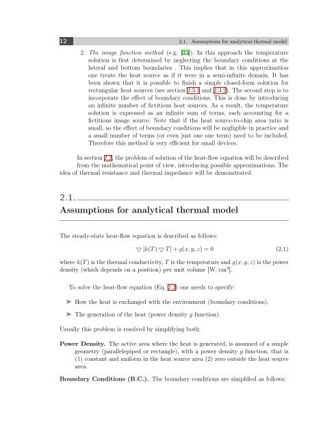
12 2.1. Assumptions <strong>for</strong> analytical <strong>thermal</strong> model<br />
2. The image function method (e.g. [35]). In this approach the temperature<br />
solution is first determined by neglecting the boundary conditions at the<br />
lateral and bottom boundaries . This implies that in this approximation<br />
one treats the heat source as if it were in a semi-infinite domain. It has<br />
been shown that it is possible to finish a simple closed-<strong>for</strong>m solution <strong>for</strong><br />
rectangular heat sources (see section 2.3.1 and 2.3.2). The second step is to<br />
incorporate the effect <strong>of</strong> boundary conditions. This is done by introducing<br />
an infinite number <strong>of</strong> fictitious heat sources. As a result, the temperature<br />
solution is expressed as an infinite sum <strong>of</strong> terms, each accounting <strong>for</strong> a<br />
fictitious image source. Note that if the heat source-to-chip area ratio is<br />
small, so the effect <strong>of</strong> boundary conditions will be negligible in practice and<br />
a small number <strong>of</strong> terms (or even just one one term) need to be included.<br />
There<strong>for</strong>e this method is very efficient <strong>for</strong> small devices.<br />
In section 2.2, the problem <strong>of</strong> solution <strong>of</strong> the heat-flow equation will be described<br />
from the mathematical point <strong>of</strong> view, introducing possible approximations. The<br />
idea <strong>of</strong> <strong>thermal</strong> resistance and <strong>thermal</strong> impedance will be demonstrated.<br />
2.1.<br />
Assumptions <strong>for</strong> analytical <strong>thermal</strong> model<br />
The steady-state heat-flow equation is described as follows:<br />
▽ [k(T ) ▽ T ] + g(x, y, z) = 0 (2.1)<br />
where k(T ) is the <strong>thermal</strong> conductivity, T is the temperature and g(x, y, z) is the power<br />
density (which depends on a position) per unit volume [W/cm 3 ].<br />
To solve the heat-flow equation (Eq. 2.2) one needs to specify:<br />
➤ How the heat is exchanged with the environment (boundary conditions).<br />
➤ The generation <strong>of</strong> the heat (power density g function).<br />
Usually this problem is resolved by simplifying both:<br />
Power Density. The active area where the heat is generated, is assumed <strong>of</strong> a simple<br />
geometry (parallelepiped or rectangle), with a power density g function, that is<br />
(1) constant and uni<strong>for</strong>m in the heat source area (2) zero outside the heat source<br />
area.<br />
Boundary Conditions (B.C.). The boundary conditions are simplified as follows: