Development of a New Electro-thermal Simulation Tool for RF circuits

32 2.4. Compact Thermal Model
Comparing the results for the generated CTM and 3D detailed model (COMSOL), a
small error is still acceptable. Nevertheless, if extreme cooling conditions are applied on
the three surfaces simultaneously, an error becomes above 10% and the results become
meaningless. It is a consequence of the assumption, the thermal resistance values follow
the linear characteristic (Fig. 2.19) with boundary condition changes.
Nonlinear control equations
It is possible to reduce the abovementioned error by adapting the control equations.
The thermal resistance values do not actually evolve linearly as it has been assumed
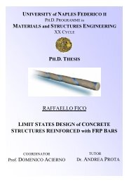
above. Fig. 2.20 shows the results for Rbottom for conditions between the two points.
The curve shape would depend on the geometry of the studied structure and the value
of applied convection. Although in many cases the linearity of contributions might be
Figure 2.20: Actual Rth_bottom compared to linear assumption.
a very good approximation, some complexity can be added to the extraction procedure
in order to obtain a much more precise model.
A series of 3D simulations have been carried out, the results fit well with the
following law:
a
∆Rth =
Px b +
c (2.54)
Ptotal
Then, the resistance definitions will be as follows instead of those in Eq. 2.51a:
Rth_T op =
Rth_Side =
Rth_Bottom =
aT −T B
cT −T B
Pbottom
bT −T B + Ptotal
+
aT - TS
cT −T S
Pside
bT −T S + Ptotal
− Rtop_ min (2.55a)
aS−SB
Pbottom
bS−SB + Ptotal
aB−BT
Ptop
bB−BT + Ptotal
cS−SB +
cB−BT +
aS - ST
cS - ST
Ptop
bS−ST + Ptotal
− Rside_ min (2.55b)
aB−BS
Pside
bB−BS + Ptotal
cB−BS − Rbottom_ min (2.55c)