booklet format - inaf iasf bologna

Temporal Data Analysis A.A. 2011/2012
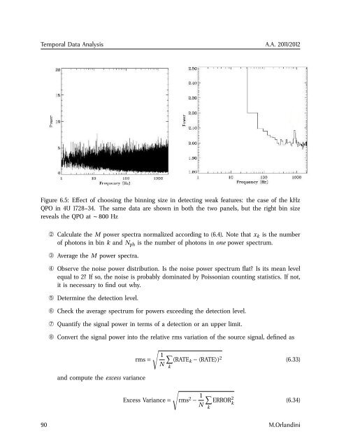
Figure 6.5: Effect of choosing the binning size in detecting weak features: the case of the kHz
QPO in 4U 1728–34. The same data are shown in both the two panels, but the right bin size
reveals the QPO at ∼ 800 Hz
➁ Calculate the M power spectra normalized according to (6.4). Note that x k is the number
of photons in bin k and N ph is the number of photons in one power spectrum.
➂ Average the M power spectra.
➃ Observe the noise power distribution. Is the noise power spectrum flat? Is its mean level
equal to 2? If so, the noise is probably dominated by Poissonian counting statistics. If not,
it is necessary to find out why.
➄ Determine the detection level.
➅ Check the average spectrum for powers exceeding the detection level.
➆ Quantify the signal power in terms of a detection or an upper limit.
➇ Convert the signal power into the relative rms variation of the source signal, defined as
and compute the excess variance
√
1 ∑
rms = (RATE k − 〈RATE〉) 2 (6.33)
N
k
√
Excess Variance = rms 2 − 1 ∑
ERROR 2 (6.34)
N
k
90 M.Orlandini
k