booklet format - inaf iasf bologna

A.A. 2011/2012
Temporal Data Analysis
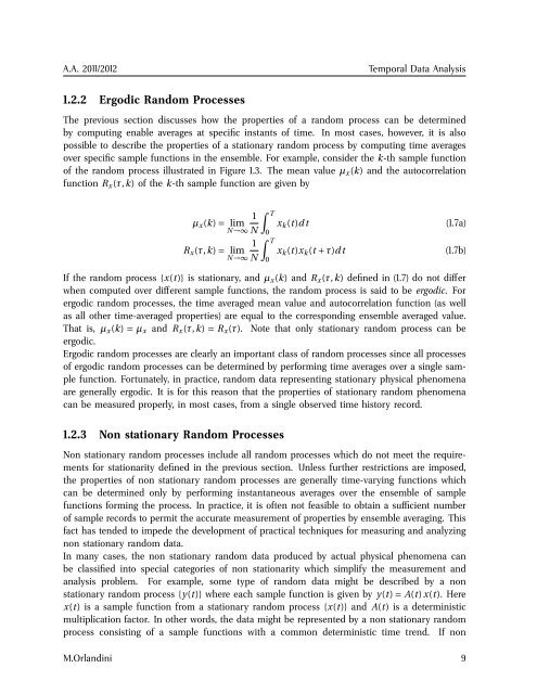
1.2.2 Ergodic Random Processes
The previous section discusses how the properties of a random process can be determined
by computing enable averages at specific instants of time. In most cases, however, it is also
possible to describe the properties of a stationary random process by computing time averages
over specific sample functions in the ensemble. For example, consider the k-th sample function
of the random process illustrated in Figure 1.3. The mean value µ x (k) and the autocorrelation
function R x (τ,k) of the k-th sample function are given by
∫
1 T
µ x (k) = lim x k (t)dt
N→∞ N 0
∫
1 T
R x (τ,k) = lim x k (t)x k (t + τ)dt
N→∞ N
0
(1.7a)
(1.7b)
If the random process {x(t)} is stationary, and µ x (k) and R x (τ,k) defined in (1.7) do not differ
when computed over different sample functions, the random process is said to be ergodic. For
ergodic random processes, the time averaged mean value and autocorrelation function (as well
as all other time-averaged properties) are equal to the corresponding ensemble averaged value.
That is, µ x (k) = µ x and R x (τ,k) = R x (τ). Note that only stationary random process can be
ergodic.
Ergodic random processes are clearly an important class of random processes since all processes
of ergodic random processes can be determined by performing time averages over a single sample
function. Fortunately, in practice, random data representing stationary physical phenomena
are generally ergodic. It is for this reason that the properties of stationary random phenomena
can be measured properly, in most cases, from a single observed time history record.
1.2.3 Non stationary Random Processes
Non stationary random processes include all random processes which do not meet the requirements
for stationarity defined in the previous section. Unless further restrictions are imposed,
the properties of non stationary random processes are generally time-varying functions which
can be determined only by performing instantaneous averages over the ensemble of sample
functions forming the process. In practice, it is often not feasible to obtain a sufficient number
of sample records to permit the accurate measurement of properties by ensemble averaging. This
fact has tended to impede the development of practical techniques for measuring and analyzing
non stationary random data.
In many cases, the non stationary random data produced by actual physical phenomena can
be classified into special categories of non stationarity which simplify the measurement and
analysis problem. For example, some type of random data might be described by a non
stationary random process {y(t)} where each sample function is given by y(t) = A(t) x(t). Here
x(t) is a sample function from a stationary random process {x(t)} and A(t) is a deterministic
multiplication factor. In other words, the data might be represented by a non stationary random
process consisting of a sample functions with a common deterministic time trend. If non
M.Orlandini 9