booklet format - inaf iasf bologna

Temporal Data Analysis A.A. 2011/2012
C k . A comparison between (2.21) and (2.20) demonstrates the two-sided character of the two
Shifting Rules. If a is an integer, there won’t be any problem if you simply take the coefficient
shifted by a. But what if a is not an integer?
Strangely enough nothing serious will happen. Simply shifting like we did before won’t work
any more, but who is to keep us from inserting (k − a) into the expression for old C k , whenever
k occurs.
Before we present examples, two more ways of writing down the Second Shifting Rule are in
order:
f (t) ↔{A k ;B k ;ω k }
f (t)e i 2πa t 1
T ↔{
2 [A k+a + A k−a + i (B k+a − B k−a )];
}
1
2 [B k+a − B k−a + i (A k−a − A k+a )];ω k
(2.22)
Caution! This is valid for k ≠ 0. Note that old A 0 becomes A a /2+iB a /2. The formulas becomes
a lot simpler in case f (t) is real. In this case we get:
old A 0 becomes A a /2 and
old A 0 becomes B a /2.
f (t) cos 2πat
T
f (t) sin 2πat
T
{
Ak+a + A k−a
↔
2
; B }
k+a + Bk − a
;ω k
2
{
Bk+a − Bk − a
↔
; A }
k+a − A k−a
;ω k
2
2
(2.23)
(2.24)
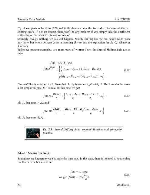
Ex. 2.3 Second Shifting Rule: constant function and triangular
function
2.1.5.3 Scaling Theorem
Sometimes we happen to want to scale the time axis. In this case, there is no need to re-calculate
the Fourier coefficients. From:
f (t) ↔ {C k ;ω k }
we get: f (at) ↔ {C k ; ω k
a } (2.25)
20 M.Orlandini