booklet format - inaf iasf bologna

A.A. 2011/2012
Temporal Data Analysis
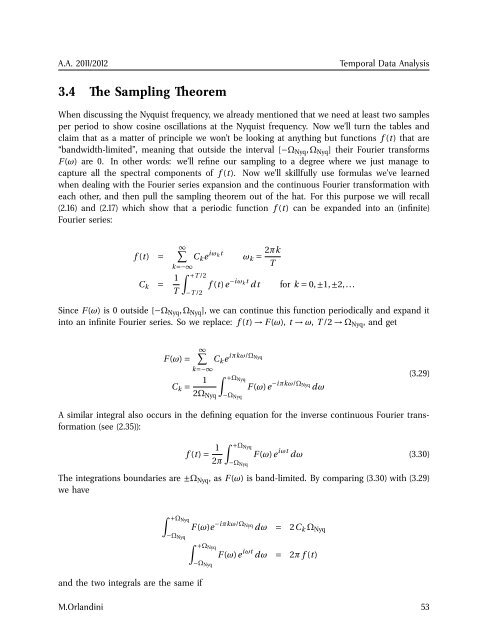
3.4 The Sampling Theorem
When discussing the Nyquist frequency, we already mentioned that we need at least two samples
per period to show cosine oscillations at the Nyquist frequency. Now we’ll turn the tables and
claim that as a matter of principle we won’t be looking at anything but functions f (t) that are
“bandwidth-limited”, meaning that outside the interval [−Ω Nyq ,Ω Nyq ] their Fourier transforms
F (ω) are 0. In other words: we’ll refine our sampling to a degree where we just manage to
capture all the spectral components of f (t). Now we’ll skillfully use formulas we’ve learned
when dealing with the Fourier series expansion and the continuous Fourier transformation with
each other, and then pull the sampling theorem out of the hat. For this purpose we will recall
(2.16) and (2.17) which show that a periodic function f (t) can be expanded into an (infinite)
Fourier series:
f (t) =
C k = 1 T
∞∑
C k e iω k t
k=−∞
∫ +T /2
−T /2
ω k = 2πk
T
f (t)e −iω k t dt for k = 0,±1,±2,...
Since F (ω) is 0 outside [−Ω Nyq ,Ω Nyq ], we can continue this function periodically and expand it
into an infinite Fourier series. So we replace: f (t) → F (ω), t → ω, T /2 → Ω Nyq , and get
∞∑
F (ω) = C k e iπkω/Ω Nyq
k=−∞
C k = 1 ∫ +ΩNyq
F (ω)e −iπkω/Ω Nyq
dω
2Ω Nyq
−Ω Nyq
(3.29)
A similar integral also occurs in the defining equation for the inverse continuous Fourier transformation
(see (2.35)):
f (t) = 1 ∫ +ΩNyq
F (ω)e iωt dω (3.30)
2π −Ω Nyq
The integrations boundaries are ±Ω Nyq , as F (ω) is band-limited. By comparing (3.30) with (3.29)
we have
∫ +ΩNyq
and the two integrals are the same if
−Ω Nyq
F (ω)e −iπkω/Ω Nyq
dω
∫ +ΩNyq
= 2C k Ω Nyq
−Ω Nyq
F (ω)e iωt dω = 2π f (t)
M.Orlandini 53