booklet format - inaf iasf bologna

A.A. 2011/2012
Temporal Data Analysis
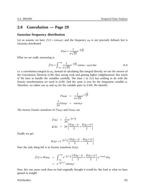
2.6 Convolution — Page 29
Gaussian frequency distribution
Let us assume we have f (t) = cosω 0 t, and the frequency ω 0 is not precisely defined, but is
Gaussian distributed:
What we are really measuring is
P(ω) = 1
σ 1 ω 2
2π e− 2 σ 2
∫ +∞
f ¯
1
(t) =
−∞ σ 1 ω 2
2π e− 2 σ 2 cos(ω − ω 0 )t dω (A.1)
i.e. a convolution integral in ω 0 . Instead of calculating this integral directly, we use the inverse of
the Convolution Theorem (2.49), thus saving work and gaining higher enlightenment. But watch
it! We have to handle the variables carefully. The time t in (A.1) has nothing to do with the
Fourier transformation we need in (2.49). And the same is true for the integration variable ω.
Therefore, we rather use t 0 and ω 0 for the variable pairs in (2.49). We identify:
F (ω 0 ) =
1
σ 1 ω 2 0
2π e− 2 σ 2
1
2π G(ω 0) = cosω 0 t
The inverse Fourier transform of F (ω 0 ) and G(ω 0 ) are
Finally we get:
f (t 0 ) = 1 1 2π e− 2 σ2 t0
2
[ δ(t0 − t)
g (t 0 ) = 2π
2
h(t 0 ) = e − 1 2 σ2 t 2 0
[ δ(t0 − t)
Now the only thing left is to Fourier transform h(t 0 ):
¯ f (t) ≡ H(ω 0 ) =
∫ +∞
e − 1 2 σ2 t0
2
−∞
= e − 1 2 σ2 t 2 cosω 0 t
2
[ δ(t0 − t)
2
+ δ(t ]
0 + t)
2
+ δ(t ]
0 + t)
2
+ δ(t ]
0 + t)
e −iω 0t 0
dt 0
2
Now, this was more work than we had originally thought it would be. But look at what we have
gained in insight!
M.Orlandini 123