booklet format - inaf iasf bologna

Temporal Data Analysis A.A. 2011/2012
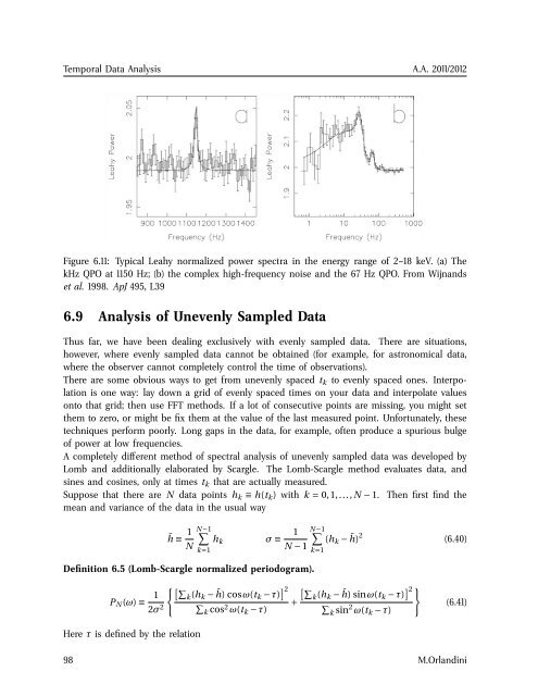
Figure 6.11: Typical Leahy normalized power spectra in the energy range of 2–18 keV. (a) The
kHz QPO at 1150 Hz; (b) the complex high-frequency noise and the 67 Hz QPO. From Wijnands
et al. 1998. ApJ 495, L39
6.9 Analysis of Unevenly Sampled Data
Thus far, we have been dealing exclusively with evenly sampled data. There are situations,
however, where evenly sampled data cannot be obtained (for example, for astronomical data,
where the observer cannot completely control the time of observations).
There are some obvious ways to get from unevenly spaced t k to evenly spaced ones. Interpolation
is one way: lay down a grid of evenly spaced times on your data and interpolate values
onto that grid; then use FFT methods. If a lot of consecutive points are missing, you might set
them to zero, or might be fix them at the value of the last measured point. Unfortunately, these
techniques perform poorly. Long gaps in the data, for example, often produce a spurious bulge
of power at low frequencies.
A completely different method of spectral analysis of unevenly sampled data was developed by
Lomb and additionally elaborated by Scargle. The Lomb-Scargle method evaluates data, and
sines and cosines, only at times t k that are actually measured.
Suppose that there are N data points h k ≡ h(t k ) with k = 0,1,..., N − 1. Then first find the
mean and variance of the data in the usual way
¯h ≡ 1 N
N−1 ∑
k=1
h k σ ≡ 1 N−1 ∑
N − 1
k=1
(h k − ¯h) 2 (6.40)
Definition 6.5 (Lomb-Scargle normalized periodogram).
{[∑
P N (ω) ≡ 1 k(h k − ¯h) cosω(t k − τ) ] 2
2σ 2 ∑
k cos 2 +
ω(t k − τ)
[∑k(h k − ¯h) sinω(t k − τ) ] 2
}
∑
k sin 2 ω(t k − τ)
(6.41)
Here τ is defined by the relation
98 M.Orlandini