booklet format - inaf iasf bologna
booklet format - inaf iasf bologna
booklet format - inaf iasf bologna

You also want an ePaper? Increase the reach of your titles
YUMPU automatically turns print PDFs into web optimized ePapers that Google loves.
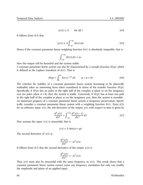
Temporal Data Analysis A.A. 2011/2012<br />
It follows from (4.3) that<br />
|x(t)| ≤ A for all t (4.4)<br />
|y(t)| ≤ A<br />
∫ +∞<br />
−∞<br />
|h(τ)|dτ (4.5)<br />
Hence if the constant parameter linear weighting function h(τ) is absolutely integrable, that is<br />
∫ +∞<br />
−∞<br />
|h(τ)|dτ < ∞<br />
then the output will be bounded and the system stable.<br />
A constant parameter linear system can also be characterized by a transfer function H(p), which<br />
is defined as the Laplace transform of h(τ). That is<br />
H(p) =<br />
∫ ∞<br />
0<br />
h(τ)e −pτ dτ p = a + ib (4.6)<br />
The criterion for stability of a constant parameter linear system (assuming to be physically<br />
realizable) takes an interesting form when considered in terms of the transfer function H(p).<br />
Specifically, if H(p) has no poles in the right half of the complex p plane or on the imaginary<br />
axis (no poles when a > 0), then the system is stable. Conversely, if H(p) has at least one pole<br />
in the right half of the complex p plane or on the imaginary axis, then the system is unstable.<br />
An important property of a constant parameter linear system is frequency preservation. Specifically,<br />
consider a constant parameter linear system with a weighting function h(τ). From (4.1),<br />
for an arbitrary input x(t), the nth derivative of the output y(t) with respect to time is given by<br />
Now assume the input x(t) is sinusoidal, that is<br />
d n ∫<br />
y(t) +∞<br />
d n x(t − τ)<br />
dt n =<br />
−∞ dt n dτ (4.7)<br />
The second derivative of x(t) is<br />
x(t) = X sin(ωt + ϕ)<br />
d 2 x(t)<br />
dx 2 = −ω 2 x(t)<br />
It follows from (4.7) that the second derivative of the output y(t) is<br />
d 2 y(t)<br />
dx 2 = −ω 2 y(t)<br />
Thus y(t) must also be sinusoidal with the same frequency as x(t). This result shows that a<br />
constant parameter linear system cannot cause any frequency translation but only can modify<br />
the amplitude and phase of an applied input.<br />
64 M.Orlandini