booklet format - inaf iasf bologna
booklet format - inaf iasf bologna
booklet format - inaf iasf bologna
Create successful ePaper yourself
Turn your PDF publications into a flip-book with our unique Google optimized e-Paper software.
A.A. 2011/2012<br />
Temporal Data Analysis<br />
Proof.<br />
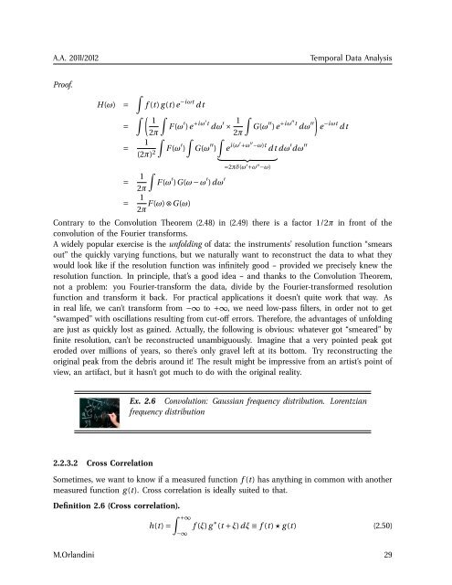
H(ω) =<br />
=<br />
=<br />
∫<br />
f (t) g (t)e −iωt dt<br />
∫ ( ∫ 1<br />
F (ω ′ )e +iω′t dω ′ × 1 ∫<br />
)<br />
G(ω ′′ )e +iω′′t dω ′′ e −iωt dt<br />
2π<br />
2π<br />
∫ ∫ ∫<br />
1<br />
(2π) 2 F (ω ′ ) G(ω ′′ ) e i (ω′ +ω ′′ −ω)t dt dω ′ dω ′′<br />
= 1 ∫<br />
2π<br />
F (ω ′ )G(ω − ω ′ )dω ′<br />
= 1 F (ω) ⊗G(ω)<br />
2π<br />
} {{ }<br />
=2πδ(ω ′ +ω ′′ −ω)<br />
Contrary to the Convolution Theorem (2.48) in (2.49) there is a factor 1/2π in front of the<br />
convolution of the Fourier transforms.<br />
A widely popular exercise is the unfolding of data: the instruments’ resolution function “smears<br />
out” the quickly varying functions, but we naturally want to reconstruct the data to what they<br />
would look like if the resolution function was infinitely good – provided we precisely knew the<br />
resolution function. In principle, that’s a good idea – and thanks to the Convolution Theorem,<br />
not a problem: you Fourier-transform the data, divide by the Fourier-transformed resolution<br />
function and transform it back. For practical applications it doesn’t quite work that way. As<br />
in real life, we can’t transform from −∞ to +∞, we need low-pass filters, in order not to get<br />
“swamped” with oscillations resulting from cut-off errors. Therefore, the advantages of unfolding<br />
are just as quickly lost as gained. Actually, the following is obvious: whatever got “smeared” by<br />
finite resolution, can’t be reconstructed unambiguously. Imagine that a very pointed peak got<br />
eroded over millions of years, so there’s only gravel left at its bottom. Try reconstructing the<br />
original peak from the debris around it! The result might be impressive from an artist’s point of<br />
view, an artifact, but it hasn’t got much to do with the original reality.<br />
Ex. 2.6 Convolution: Gaussian frequency distribution. Lorentzian<br />
frequency distribution<br />
2.2.3.2 Cross Correlation<br />
Sometimes, we want to know if a measured function f (t) has anything in common with another<br />
measured function g (t). Cross correlation is ideally suited to that.<br />
Definition 2.6 (Cross correlation).<br />
h(t) =<br />
∫ +∞<br />
−∞<br />
f (ξ) g ∗ (t + ξ)dξ ≡ f (t) ⋆ g (t) (2.50)<br />
M.Orlandini 29


