- Page 1 and 2:
Mitglied Mitglied der der Helmholtz
- Page 4 and 5:
Forschungszentrum Jülich GmbH Inst
- Page 6 and 7:
TABLE OF CONTENTS 1 Preface .......
- Page 8:
6.2.2 Doctoral Thesis .............
- Page 11 and 12:
state of NRW. The collaborative pro
- Page 13 and 14:
2 Institute’s Profile Due to the
- Page 15 and 16:
2.2. Organization chart Reactor Saf
- Page 17 and 18:
3 Key Research Topics 3.1. Long Ter
- Page 19 and 20:
actinide co-conversion into polyact
- Page 21 and 22:
Fig. 7: Non-destructive analytical
- Page 23 and 24:
Fig. 9: Thermal treatment of an AVR
- Page 25 and 26:
3.8. Product Quality Control of Rad
- Page 27 and 28:
3.8.2 Product Quality Control of Lo
- Page 29 and 30:
The advantage of working at low vac
- Page 31 and 32:
NdPO 4 powder sample, directly rece
- Page 33 and 34:
4.5. Non-destructive assay testing
- Page 35 and 36:
5 Scientific and Technical Reports
- Page 37 and 38:
Results and Discussion The irradiat
- Page 39 and 40:
work will focus on the identificati
- Page 41 and 42:
Different solvents (iso-propanol an
- Page 43 and 44:
e & j) Aggregates of aluminium oxid
- Page 45 and 46:
Experimental details The corrosion
- Page 47 and 48:
Intensity [CPS] 500 400 300 200 100
- Page 49 and 50:
Fig. 24: Left: High resolution TEM
- Page 51 and 52:
a) MD model [10] b) Derived Lesukit
- Page 53 and 54:
5.4. Minor actinide(III) recovery f
- Page 55 and 56:
Extensive extraction studies were p
- Page 57 and 58:
of the extraction properties of the
- Page 59 and 60:
Cm(III) together with the lanthanid
- Page 61 and 62:
using a mixture of CyMe4BTBP and TO
- Page 63 and 64:
A more challenging route studied wi
- Page 65 and 66:
These preliminary results show that
- Page 67 and 68:
The 1-cycle SANEX process is intend
- Page 69 and 70:
Continuous counter-current tests us
- Page 71 and 72:
Conclusion In this work, it was sho
- Page 73 and 74:
shaken by a vortex mixer for 15 min
- Page 75 and 76: 100 100 Distribution ratio 10 1 0.1
- Page 77 and 78: Tab. 15: The distribution ratios of
- Page 79 and 80: 5.7. Synthesis and thermal treatmen
- Page 81 and 82: Acid-Deficient Uranyl-Nitrate via d
- Page 83 and 84: Optical investigation showed a noti
- Page 85 and 86: TG /% 100 98 96 94 92 90 88 86 84 8
- Page 87 and 88: Radiolysis in the aqueous solutions
- Page 89 and 90: is about 4% while the one of the rh
- Page 91 and 92: Fig. 59: Compressibility curve for
- Page 93 and 94: Conclusion and outlook Monazite-typ
- Page 95 and 96: Fig. 63: Description of the unit ce
- Page 97 and 98: agents for the synthesis of neodymi
- Page 99 and 100: 100 TG 785°C Exo DSC 0,2 0,0 90 -0
- Page 101 and 102: After synthesis the product was cen
- Page 103 and 104: process of monazite and additional
- Page 105 and 106: Tab. 18: Lattice parameters determi
- Page 107 and 108: Conclusions For Sm 1-x Ce x PO 4 mo
- Page 109 and 110: 5.11. Raman Spectra of Synthetic Ra
- Page 111 and 112: The numerical values of all measure
- Page 113 and 114: knowledge, these special relationsh
- Page 115 and 116: Fig. 80: Raman spectra of LaPO 4 ir
- Page 117 and 118: 5.12. MC simulation of thermal neut
- Page 119 and 120: content was replaced by hydrogen. C
- Page 121 and 122: constant for hydrogen concentration
- Page 123 and 124: with a 0 1 -183.88 ± 8.55 and a 2
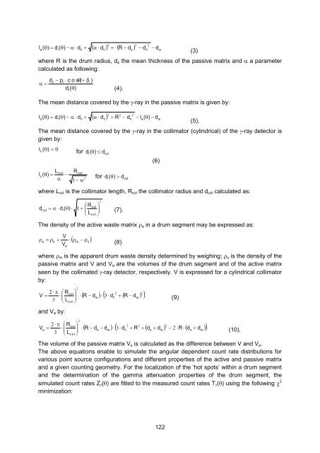
- Page 125: 5.13. An Improved Method for the no
- Page 129 and 130: The relative uncertainty for the ac
- Page 131 and 132: In the drum, 4 ‘hot spots’ for
- Page 133 and 134: activity of Cs-137 is much more und
- Page 135 and 136: gamma-ray detector approximated by
- Page 137 and 138: shown in Fig. 96. In both cases the
- Page 139 and 140: econstruction than the old calculat
- Page 141 and 142: Neutron capture cross sections and
- Page 143 and 144: Outlook The evaluated data will be
- Page 145 and 146: from carbon-based HTR fuel elements
- Page 147 and 148: Fig. 102: 3D volume reconstructions
- Page 149 and 150: dislocate the 14 C atom from its pr
- Page 151 and 152: It can be seen that nearly all trit
- Page 153 and 154: Acknowledgement The authors like to
- Page 155 and 156: development by investigations of ga
- Page 157 and 158: Fig. 109: The left picture shows th
- Page 159 and 160: [2] A European Roadmap for Developi
- Page 161 and 162: from airborne SWIR Full Spectrum Im
- Page 163 and 164: Fig. 113: Visualization of the vege
- Page 165 and 166: number of training samples up to 19
- Page 167 and 168: Acknowledgements The work presented
- Page 169 and 170: three approaches has severe drawbac
- Page 171 and 172: neighbours from the list of merge c
- Page 173 and 174: it gives a difference in segmentati
- Page 175 and 176: [6] I. Niemeyer, F. Bachmann, A. Jo
- Page 177 and 178:
Monitoring 3 cooperated intensively
- Page 179 and 180:
facilities and other treaty related
- Page 181 and 182:
parameters of the SAR system, such
- Page 183 and 184:
The MGD products used in the study
- Page 185 and 186:
Fig. 134 contains the result for th
- Page 187 and 188:
[2] H. Maître (ed.), Processing of
- Page 189 and 190:
Preparatory Committee to allocate t
- Page 191 and 192:
unconditional security assurances f
- Page 193 and 194:
safeguards was also requested. Deci
- Page 195 and 196:
[16] United Nations Security Counci
- Page 197 and 198:
5.24. Development and Application o
- Page 199 and 200:
Hardware layer The hardware layer i
- Page 201 and 202:
So in most applications the scale u
- Page 203 and 204:
The ENDF-B/V and ENDF-B/VI librarie
- Page 205 and 206:
5.26. Product control of waste prod
- Page 207 and 208:
Polysiloxane which has been investi
- Page 209 and 210:
acceptance requirements [3]. In the
- Page 211 and 212:
Fig. 145: List of description and d
- Page 213 and 214:
6.1. Courses taught at universities
- Page 215 and 216:
Umwelt / Energy & Environment 2010;
- Page 217 and 218:
6.5. Institute Seminar The IEK-6 or
- Page 219 and 220:
6.5.3 Invited talks 2009 30.04.2009
- Page 221 and 222:
21.09.2010 Dr. N. Evans: The Chemis
- Page 223 and 224:
8 Selected R&D projects 8.1. EU pro
- Page 225 and 226:
K. Aymanns: Nominated as deputy re
- Page 227 and 228:
Bukaemskiy A.A., Barrier D., Modolo
- Page 229 and 230:
11.2. Publications 2009 11.2.1 Jour
- Page 231 and 232:
Rezniczek, A.; Richter, B.; Jussofi
- Page 233 and 234:
Daniels, H.: Co-conversion of actin
- Page 235 and 236:
11.3. Publications 2010 11.3.1 Jour
- Page 237 and 238:
Sypula, M.; Wilden, A.; Schreinemac
- Page 239 and 240:
(Partitioning) - Stabilitätsunters
- Page 241 and 242:
Modolo, G.; Bosbach, D.; Geist, A.;
- Page 243 and 244:
12 How to reach us Postal Address F
- Page 245 and 246:
By train: Take the train from Aache
- Page 247 and 248:
Schriften des Forschungszentrums J
- Page 249 and 250:
Schriften des Forschungszentrums J
- Page 251 and 252:
Schriften des Forschungszentrums J
- Page 253 and 254:
Schriften des Forschungszentrums J
- Page 255 and 256:
Schriften des Forschungszentrums J
- Page 257 and 258:
Schriften des Forschungszentrums J
- Page 259:
Schriften des Forschungszentrums J