Numerical Methods in Quantum Mechanics - Dipartimento di Fisica

More documents

Recommendations

Info

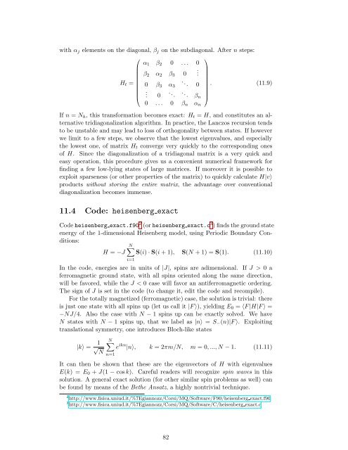
with α j elements on the diagonal, β j on the subdiagonal. After n steps: ⎛ ⎞ α 1 β 2 0 . . . 0 β 2 α 2 β 3 0 . H t = . 0 β 3 α .. 3 0 . (11.9) ⎜ . ⎝ . 0 .. . .. ⎟ βn ⎠ 0 . . . 0 β n α n If n = N h , this transformation becomes exact: H t = H, and constitutes an alternative tridiagonalization algorithm. In practice, the Lanczos recursion tends to be unstable and may lead to loss of orthogonality between states. If however we limit to a few steps, we observe that the lowest eigenvalues, and especially the lowest one, of matrix H t converge very quickly to the corresponding ones of H. Since the diagonalization of a tridiagonal matrix is a very quick and easy operation, this procedure gives us a convenient numerical framework for finding a few low-lying states of large matrices. If moreover it is possible to exploit sparseness (or other properties of the matrix) to quickly calculate H|v〉 products without storing the entire matrix, the advantage over conventional diagonalization becomes immense. 11.4 Code: heisenberg exact Code heisenberg exact.f90 2 (or heisenberg exact.c 3 ) finds the ground state energy of the 1-dimensional Heisenberg model, using Periodic Boundary Conditions: N∑ H = −J S(i) · S(i + 1), S(N + 1) = S(1). (11.10) i=1 In the code, energies are in units of |J|, spins are adimensional. If J > 0 a ferromagnetic ground state, with all spins oriented along the same direction, will be favored, while the J < 0 case will favor an antiferromagnetic ordering. The sign of J is set in the code (to change it, edit the code and recompile). For the totally magnetized (ferromagnetic) case, the solution is trivial: there is just one state with all spins up (let us call it |F 〉), yielding E 0 = 〈F |H|F 〉 = −NJ/4. Also the case with N − 1 spins up can be exactly solved. We have N states with N − 1 spins up, that we label as |n〉 = S − (n)|F 〉. Exploiting translational symmetry, one introduces Bloch-like states |k〉 = 1 √ N N ∑ n=1 e ikn |n〉, k = 2πm/N, m = 0, ..., N − 1. (11.11) It can then be shown that these are the eigenvectors of H with eigenvalues E(k) = E 0 + J(1 − cos k). Careful readers will recognize spin waves in this solution. A general exact solution (for other similar spin problems as well) can be found by means of the Bethe Ansatz, a highly nontrivial technique. 2 http://www.fisica.uniud.it/%7Egiannozz/Corsi/MQ/Software/F90/heisenberg exact.f90 3 http://www.fisica.uniud.it/%7Egiannozz/Corsi/MQ/Software/C/heisenberg exact.c 82
The code requires the number N of spins and the number nup of up spins, computes the dimension nhil of the Hilbert space. It then proceeds to the labeling of the states, using a trick often employed for spin-1/2 systems: an integer index k, running from 1 to 2 N −1, contains in its i−th bit the information (0=down, 1=up) for the i−th spin. Of course this works only up to 32 spins, for default integers (or 64 spins for INTEGER(8)). The integer k is stored into array states for the states in the required Hilbert space. The Hamiltonian matrix is then filled (the code does not takes advantage of sparseness) and the number of nonzero matrix elements counted. For the S + S − and S − S + terms in the Hamiltonian, only matrix elements as in 11.5 and 11.6, respectively, are calculated. We remark that the line k = states(ii)+2**(j-1)-2**(i-1) is a quick-and-dirty way to calculate the index for the state obtained by flipping down spin i and flipping up spin j in state states(ii). 4 We then proceed to the generation of the Lanczos chain. The number nl of chain steps (should not exceed nhil) is prompted for and read from terminal. The starting vector is filled with random numbers. Note the new BLAS routines dnrm2 and dgemv: the former calculates the module of a vector, the latter a matrix-vector product and is used to calculate H|v〉. The Hamiltonian in tridiagonal form (contained in the two arrays d and e) is then diagonalized by the LAPACK routine dsterf, that actually finds only the eigenvalues. The lowest eigenvalues is then printed for increasing values of the dimension of the tridiagonal matrix, up to nl, so that the convergence of the Lanczos chain can be estimated. You can modify the code to print more eigenvalues. As a final check, the matrix is diagonalized using the conventional algorithm (routine dspev). Note how much slower this final step is than the rest of the calculation! Once you are confident that the Lanczos chain works, you can speed up the calculations by commenting out the exact diagonalization step. The limiting factor will become the size of the Hamiltonian matrix. 11.4.1 Computer Laboratory • Examine the convergence of the Lanczos procedure to the exact energy • For the antiferromagnetic case, verify that the ground state has zero magnetization. Plot the ground-state energy E 0 and the first excited state E 1 as a function of N. Try to verify if the gap E − E 0 has a 1/N dependence. • For the ferromagnetic case, verify that the ground state has all spins aligned. Note that the ground state will have the same energy no matter what total magnetization you choose! This is a consequence of the rotational invariance of the Heisenberg Hamiltonian. Verify that the case with N − 1 spins up corresponds to the spin-wave solution, Eq.(11.11). You will need to print all eigenvalues. 4 A more elegant but hardly more transparent way would be to directly manipulate the corresponding bits. 83
Page 1 and 2:
Lecture notes Numerical Methods in
Page 3 and 4:
3.3 Code: crossection . . . . . . .
Page 5 and 6:
Introduction The aim of these lectu
Page 7 and 8:
is an important and well-known libr
Page 9 and 10:
Chapter 1 One-dimensional Schrödin
Page 11 and 12:
Under the assumption of Eq.(1.8), E
Page 13 and 14:
point its value is still ∼ 60% of
Page 15 and 16:
an equation involving finite differ
Page 17 and 18:
eigenvalue) to force the code to pe
Page 19 and 20:
1.3.3 Laboratory Here are a few hin
Page 21 and 22:
The Hamiltonian can thus be written
Page 23 and 24:
In the following we will use q 2 e
Page 25 and 26:
The dominating term close to the nu
Page 27 and 28:
whose goal is to give an estimate,
Page 29 and 30:
Chapter 3 Scattering from a potenti
Page 31 and 32:
3.2 Scattering of H atoms from rare
Page 33 and 34:
1. Solution of the radial Schrödin
Page 35 and 36: • In the limit of a weak potentia
Page 37 and 38: By modifying ψ as ψ + δψ, the e
Page 39 and 40: This demonstrates Eq.(4.19), since
Page 41 and 42: that the same equations, for a fini
Page 43 and 44: eported here are immediately genera
Page 45 and 46: BLAS 5 (collected here: dgemm.f 6 )
Page 47 and 48: known as generalized eigenvalue pro
Page 49 and 50: The Hamiltonian operator for this p
Page 51 and 52: Chapter 6 Self-consistent Field A w
Page 53 and 54: (the variations of all other normal
Page 55 and 56: nucleus. Even in open-shell atoms,
Page 57 and 58: Chapter 7 The Hartree-Fock approxim
Page 59 and 60: Now that we have the expectation va
Page 61 and 62: number of possible Slater determina
Page 63 and 64: Let us now introduce a further vari
Page 65 and 66: The index R is a reminder that both
Page 67 and 68: Molecular orbitals theory can expla
Page 69 and 70: Verify how sensitive the result is
Page 71 and 72: potential, we can hope to obtain a
Page 73 and 74: with wave vector k will be purely k
Page 75 and 76: Fast Fourier Transform In the simpl
Page 77 and 78: truncate it, it is convenient to co
Page 79 and 80: A reciprocal lattice of vectors G m
Page 81 and 82: The origin of the coordinate system
Page 83 and 84: Chapter 11 Exact diagonalization of
Page 85: The only nonzero matrix elements fo
Page 89 and 90: Appendix A From two-body to one-bod
Page 91 and 92: Appendix B Accidental degeneracy an
Page 93 and 94: and [J 2 1 , J z] = [J 2 2 , J z] =
Page 95 and 96: part and symmetric coordinate part)
Page 97 and 98: and the corresponding energy is E =
Page 99 and 100: D.3.1 Laboratory • observe the ef
Page 101: • Relative error: |a − b| < ɛa
show all

Numerical Methods in Quantum Mechanics - Dipartimento di Fisica

You also want an ePaper? Increase the reach of your titles

Delete template?

Save as template?