Multi-Objective Optimization of Wire Antennas ... - Radioengineering
Multi-Objective Optimization of Wire Antennas ... - Radioengineering
Multi-Objective Optimization of Wire Antennas ... - Radioengineering

Create successful ePaper yourself
Turn your PDF publications into a flip-book with our unique Google optimized e-Paper software.
RADIOENGINEERING, VOL. 14, NO. 4, DECEMBER 2005 91<br />
<strong>Multi</strong>-<strong>Objective</strong> <strong>Optimization</strong> <strong>of</strong> <strong>Wire</strong> <strong>Antennas</strong>:<br />
Genetic Algorithms Versus Particle Swarm <strong>Optimization</strong><br />
Zbyněk LUKEŠ, Zbyněk RAIDA<br />
Dept. <strong>of</strong> Radio Electronics, Brno University <strong>of</strong> Technology, Purkyňova 118, 612 00 Brno, Czech Republic<br />
lukes@feec.vutbr.cz, raida@feec.vutbr.cz<br />
Abstract. The paper is aimed to the multi-objective optimization<br />
<strong>of</strong> wire multi-band antennas. <strong>Antennas</strong> are numerically<br />
modeled using time-domain integral-equation method.<br />
That way, the designed antennas can be characterized<br />
in a wide band <strong>of</strong> frequencies within a single run <strong>of</strong> the<br />
analysis. <strong>Antennas</strong> are optimized to reach the prescribed<br />
matching, to exhibit the omni-directional constant gain and<br />
to have the satisfactory polarization purity. Results <strong>of</strong> the<br />
design are experimentally verified.<br />
The multi-objective cost function is minimized by the genetic<br />
algorithm and by the particle swarm optimization. Results<br />
<strong>of</strong> the optimization by both the multi-objective methods<br />
are in detail compared.<br />
The combination <strong>of</strong> the time domain analysis and global<br />
optimization methods for the broadband antenna design<br />
and the detailed comparison <strong>of</strong> the multi-objective particle<br />
swarm optimization with the multi-objective genetic algorithm<br />
are the original contributions <strong>of</strong> the paper.<br />
Keywords<br />
<strong>Wire</strong> antennas, multi-band antennas, multi-objective<br />
optimization, time-domain integral-equation method,<br />
genetic algorithms, particle swarm optimization.<br />
1. Introduction<br />
In today’s radio communication systems, broad- and<br />
multi-band antennas play more and more important role. In<br />
order to make the design <strong>of</strong> such antennas as efficient as<br />
possible, we propose to combine the time-domain integralequation<br />
(TDIE) method for the antenna analysis, and global<br />
optimization techniques for improving parameters <strong>of</strong><br />
the analyzed antenna model.<br />
If TDIE is used for the antenna analysis, the investigated<br />
antenna structure can be characterized within a single<br />
run <strong>of</strong> the analysis when excited by a very short pulse,<br />
which spectrum covers the whole frequency band <strong>of</strong> the<br />
interest [1]. Nevertheless, the TDIE suffers from stability<br />
problems in certain situations [2]–[5], and hence, its popularity<br />
is lower compared to other numerical techniques.<br />
Genetic algorithms (GA) were introduced to the computational<br />
electromagnetics like the efficient global optimization<br />
tool in the middle <strong>of</strong> nineties [6]–[8]. For the design<br />
<strong>of</strong> broad- and multi-band antennas, GA were applied in [9],<br />
[10] in conjunction with frequency domain method <strong>of</strong> moments<br />
– the analysis was run thousands times. In order to<br />
overcome this difficulty, a technique <strong>of</strong> the optimal selection<br />
<strong>of</strong> frequency points in the wide band <strong>of</strong> the design was<br />
developed [11]. Also, the first attempt to move the analysis<br />
into the time domain was published in [12] – as a computational<br />
tool, the finite-difference time-domain (FDTD)<br />
method was used.<br />
An intensive activity has been focused also on the<br />
development <strong>of</strong> multi-objective genetic optimization. In<br />
[13] and [14], the multi-objective genetic algorithm is applied<br />
to the design <strong>of</strong> broadband wire antennas using the<br />
frequency domain moment method as the computational<br />
tool. In [15], the moment method was replaced by the frequency<br />
domain finite element method combined with<br />
boundary integral equation method to design absorbers.<br />
Obviously, no so-far published approach combines TDIE<br />
and GA for multi-objective optimization <strong>of</strong> antennas.<br />
x<br />
z<br />
ϕ<br />
ϑ<br />
1<br />
1<br />
ϑ 2<br />
ϕ 2<br />
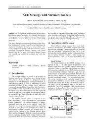
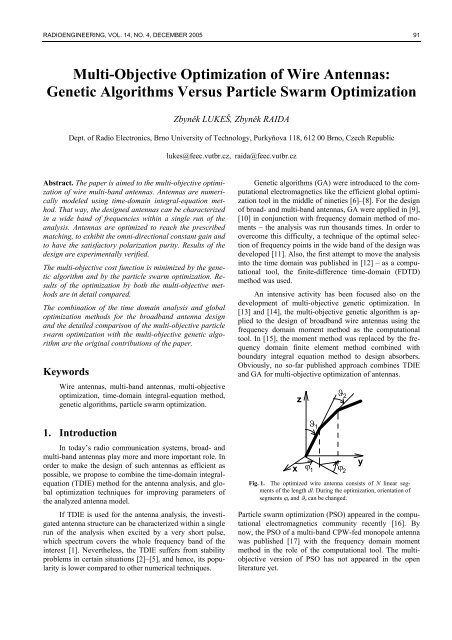
Fig. 1. The optimized wire antenna consists <strong>of</strong> N linear segments<br />
<strong>of</strong> the length dl. During the optimization, orientation <strong>of</strong><br />
segments ϕ n and ϑ n can be changed.<br />
Particle swarm optimization (PSO) appeared in the computational<br />
electromagnetics community recently [16]. By<br />
now, the PSO <strong>of</strong> a multi-band CPW-fed monopole antenna<br />
was published [17] with the frequency domain moment<br />
method in the role <strong>of</strong> the computational tool. The multiobjective<br />
version <strong>of</strong> PSO has not appeared in the open<br />
literature yet.<br />
y
92 Z. LUKEŠ, Z. RAIDA, MULTI-OBJECTIVE OPTIMIZATION OF WIRE ANTENNAS: GENETIC ALGORITHMS VERSUS ...<br />
The single-objective versions <strong>of</strong> GA and PSO were<br />
confronted in [18] when applied to the phased array synthesis.<br />
The comparison <strong>of</strong> multi-objective algorithms is<br />
published first here.<br />
The paper is organized as follows. In Section 2, the<br />
antenna to be synthesized is described. In Section 3, the<br />
techniques used (TDIE, GA, PSO) are briefly reviewed.<br />
Section 4 describes results obtained by computations, and<br />
confronts them with measurements. And finally, Section 5<br />
concludes the paper.<br />
2. Synthesized Antenna<br />
Abilities <strong>of</strong> the design technique combining the TDIE<br />
and multi-objective global optimization algorithms will be<br />
demonstrated on the synthesis <strong>of</strong> the double-band GPS antenna.<br />
The antenna consists <strong>of</strong> the arbitrarily shaped wire<br />
monopole, which is completed by the planar reflector. Both<br />
the monopole and the reflector are assumed to be perfectly<br />
electrically conductive. The antenna is surrounded by the<br />
free space with the parameters <strong>of</strong> vacuum.<br />
The antenna will operate in the frequency bands L1<br />
(the central frequency f L1 = 1575.42 MHz) and L2 (the<br />
central frequency f L2 = 1227.6 MHz). The antenna is required<br />
to exhibit the omni-directional constant gain for the<br />
elevation from 5° to 90°. The antenna has to be designed<br />
for the right-hand circular polarization.<br />
The monopole is assumed to consist <strong>of</strong> N linear segments<br />
<strong>of</strong> lengths dl n and the radius a (dl n are much longer<br />
than a, and therefore, the thin-wire approximation can be<br />
applied in the TDIE). When synthesizing the shape <strong>of</strong> the<br />
antenna, we change local spherical coordinates ϕ n , ϑ n and<br />
lengths dl n <strong>of</strong> all antenna segments. The origin <strong>of</strong> the local<br />
spherical coordinate system <strong>of</strong> the n-th antenna segment is<br />
located at the end <strong>of</strong> the (n–1) segment as depicted in Fig.<br />
1. Hence, N triplets [ϕ n , ϑ n , dl n ] are the result <strong>of</strong> the design.<br />
For the antenna optimization, three partial objective<br />
functions are formulated. The first one<br />
2<br />
1<br />
2<br />
2<br />
F<br />
f<br />
= ∑ [ Re{ Zi}<br />
−100] + [ Im{ Zi}<br />
− 0]<br />
(1)<br />
2<br />
i=<br />
1<br />
is zero if the real part <strong>of</strong> input impedance Re{Z i } = 100 Ω<br />
and the imaginary part Im{X i } = 0 Ω on central frequencies<br />
<strong>of</strong> both the frequency bands i = 1, 2.<br />
The second partial objective function<br />
2<br />
∑ [ Gmax,<br />
i<br />
− Gmin,<br />
i<br />
]<br />
F =<br />
(2)<br />
g<br />
i=<br />
1<br />
is zero in case if the maximum gain G max, i in any direction<br />
<strong>of</strong> elevation ϑ = and azimuth ϕ = <br />
equals to the minimum gain G min, i on central frequencies <strong>of</strong><br />
both the frequency bands i = 1, 2. Hence, the omni-directional<br />
constant value <strong>of</strong> the antenna gain is reached.<br />
The third partial objective function formulates the<br />
criteria <strong>of</strong> the polarization purity: the ratio (E ϕ / E ϑ ) has to<br />
equal one, and the phase shift between E ϕ and E ϑ has to be<br />
the odd multiple <strong>of</strong> π/2. If both the conditions are met on<br />
central frequencies <strong>of</strong> both the frequency bands, then the<br />
polarization purity objective function F p is zero.<br />
The partial objective functions can be joined into the<br />
global objective function<br />
F = F + F + F . (3)<br />
2<br />
f<br />
2<br />
g<br />
2<br />
p<br />
Triplets [ϕ n , ϑ n , dl n ] are changed during the optimization to<br />
reach the minimum <strong>of</strong> the global objective function F.<br />
3. Techniques Used<br />
In this Section, we briefly review the time-domain<br />
integral-equation (TDIE) method we use for evaluating the<br />
objective functions in the optimization procedure. The genetic<br />
algorithm (GA) and the particle swarm optimization<br />
(PSO) we use for minimizing objective functions are also<br />
briefly described here.<br />
3.1 Time Domain Integral Equations<br />
The method uses electric field integral equations [23]<br />
for the description <strong>of</strong> the analyzed structure. The equations<br />
are formulated for an arbitrary time response. Formulations<br />
are based on the retarded vector potential [22]<br />
( r t) = A[ J( r′<br />
, t − r − r c)<br />
]<br />
A , ′ , (4)<br />
and the retarded scalar one [22]<br />
V<br />
( r t) = V [ q( r′<br />
, t − r − r′<br />
c)<br />
]<br />
, . (5)<br />
Here, r gives the observation point (potentials are computed<br />
here) and r’ is the source point (points out to current<br />
and charge sources contributing to potentials), |r – r’| is the<br />
distance between the observation point and the source one,<br />
and c is the velocity <strong>of</strong> light in a free space. The J represents<br />
the current density vector and q is the charge density.<br />
Currents and charges are joined by the continuity theorem,<br />
and the vector potential A and the scalar one V are used to<br />
evaluate the intensity <strong>of</strong> the scattered electric field [23].<br />
In case <strong>of</strong> thin wire antennas, a so-called thin-wire<br />
approximation 1 can be introduced, which decreases the<br />
dimension <strong>of</strong> the problem. Then, the antenna segments can<br />
be represented by their axes, the axes <strong>of</strong> segments can be<br />
1<br />
If the length <strong>of</strong> the antenna segment is much smaller<br />
than the radius <strong>of</strong> the antenna wire and much smaller<br />
than the wavelength, all the currents and charges on the<br />
antenna wire can be assumed to be concentrated on the<br />
axes <strong>of</strong> antenna segments. This assumption does not<br />
agree with the reality (due to the skin effect) but provides<br />
results, which are close to measurements.
RADIOENGINEERING, VOL. 14, NO. 4, DECEMBER 2005 93<br />
broken into one-dimensional (1D) discretization cells, and<br />
the current distribution can be approximated over discretization<br />
cells using piecewise constant basis functions (on<br />
the discretization cell, the current is the same for all the<br />
points <strong>of</strong> the cell, but it can change in time).<br />
Performing several mathematical operations, an explicit<br />
formula for the current on the m-th discretization cell in<br />
the k-th time step can be obtained [22]<br />
I<br />
( m,<br />
k) κ( m,<br />
m)<br />
=<br />
− A ( m,<br />
k) + 2A<br />
( m,<br />
k −1) − A ( m,<br />
k − 2)<br />
+<br />
+<br />
1<br />
⎡c<br />
⎢<br />
⎣<br />
∆<br />
∆<br />
2<br />
t ⎤<br />
⎥<br />
⎦<br />
[ A ( m + 1, k) − 2A<br />
( m,<br />
k) + A ( m −1,<br />
k)<br />
]<br />
2<br />
( c ∆t) F ( m,<br />
k −1) ,<br />
0<br />
0<br />
where κ( m, n) denotes the integral <strong>of</strong> the time-domain<br />
Green function over the n-th discretization cell for the m-th<br />
observation point [22], A t ( m, k) is the contribution <strong>of</strong> the<br />
upcoming current samples (the moment k) to the vector<br />
potential in the centre <strong>of</strong> the m-th discretization cell, and<br />
A 1 ( m, k) is the contribution <strong>of</strong> former current samples (the<br />
moments k–1, k–2, ...) to the vector potential in the centre<br />
<strong>of</strong> the m-th discretization cell, and A 0 ( m, k) = A 1 ( m, k–1) –<br />
– A t ( m, k–1) [22]. Next, c denotes velocity <strong>of</strong> light, ∆t is<br />
the time step (the discretization segment in time), and ∆ denotes<br />
the length <strong>of</strong> the spatial discretization segment [22].<br />
Finally, the term<br />
F<br />
( m k)<br />
1<br />
=<br />
c<br />
,<br />
2<br />
I<br />
∂E<br />
∂t<br />
( m,<br />
k)<br />
describes the excitation (E I is the electric field intensity <strong>of</strong><br />
the incident wave). In our computations, antennas are excited<br />
by Gaussian pulse <strong>of</strong> the width 0.25 LM 2 . Then, antenna<br />
parameters in both the frequency bands L1 and L2 can<br />
be obtained within a single analysis.<br />
The explicit formula is stable for the time step shorter<br />
than ∆t ≤ R min / c (the minimum distance between the centers<br />
<strong>of</strong> the discretization cells R min is longer than the distance<br />
covered by light within one time step <strong>of</strong> the algorithm<br />
∆t). Meeting this condition, TDIE becomes an efficient and<br />
accurate computational tool for evaluating cost functions in<br />
our optimization.<br />
3.2 Genetic Algorithms<br />
Genetic algorithms (GA) understand the optimized<br />
antenna like an individual, which properties are described<br />
by a gene [8]. Therefore, all the state variables <strong>of</strong> the antenna,<br />
which are changed during the optimization, are binary<br />
encoded and sequentially put into a binary array – gene.<br />
2<br />
0<br />
0<br />
0<br />
+<br />
(6)<br />
+<br />
(7)<br />
The light meter (LM) equals to the time needed for covering<br />
one meter by an electromagnetic wave in free<br />
space.<br />
In order to improve the antenna parameters, a population<br />
<strong>of</strong> individuals (antennas) is randomly generated (i.e.,<br />
a set <strong>of</strong> optimized antennas differing in the setting <strong>of</strong> their<br />
state variables is created). Then, each individual in the population<br />
is evaluated (the objective function is computed<br />
for each antenna) and the best ones are selected to become<br />
parents. Couples <strong>of</strong> parents are then randomly selected [8].<br />
The cross-over operation randomly divides genes <strong>of</strong><br />
parents (a sequence <strong>of</strong> binary encoded state variables), and<br />
forms two children (the gene <strong>of</strong> the first child contains the<br />
first part <strong>of</strong> the first parent gene and the second part <strong>of</strong> the<br />
second parent gene and vice versa). That way, the population<br />
<strong>of</strong> parents is replaced by a population <strong>of</strong> children,<br />
which should exhibit better properties [8].<br />
In case <strong>of</strong> our antenna, the gene is composed <strong>of</strong> three<br />
parts: the first one contains the binary-coded elevation angles<br />
ϑ n (10 bits), the second one the binary coded azimuth<br />
angles ϕ n (10 bits), and the third one the binary coded<br />
number <strong>of</strong> the discretization elements ∆ (3 to 6) forming<br />
antenna segments dl n . The antenna consists <strong>of</strong> 7 segments.<br />
Initially, 32 binary genes were randomly generated to<br />
form the population, 32 antennas were analyzed using<br />
TDIE, and the best <strong>of</strong> them (the lowest value <strong>of</strong> the global<br />
objective function) were selected to become parents.<br />
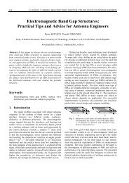
F tot<br />
iterations<br />
Fig. 2. Genetic optimization <strong>of</strong> the antenna. Comparison <strong>of</strong> different<br />
selection strategies: population decimation (solid),<br />
tournament selection (dashed), proportional selection (dashdotted).<br />
In our experiments, 3 selection strategies were tested. Population<br />
decimation selects 50 % <strong>of</strong> the best individuals to<br />
be parents (therefore, 64 individuals form the initial population<br />
in that case), and in the following steps, the better<br />
half generation overwrites the worse one. Tournament selection<br />
randomly selects couples, and the better individual<br />
in the couple is allowed to be a parent. In case <strong>of</strong> proportional<br />
selection, probability <strong>of</strong> the individual to become a<br />
parent is related to the value <strong>of</strong> its objective function (lower<br />
the objective function is, higher the probability is) [8].<br />
We also applied 10 % mutation (10 % probability that<br />
one bit randomly selected in a gene will be inverted).
94 Z. LUKEŠ, Z. RAIDA, MULTI-OBJECTIVE OPTIMIZATION OF WIRE ANTENNAS: GENETIC ALGORITHMS VERSUS ...<br />
Fig. 2 compares convergence properties <strong>of</strong> all the 3<br />
selection strategies. The convergence curves were averaged<br />
over 5 realizations <strong>of</strong> the optimization. The optimization<br />
was stopped in the 100 th iteration. Since the tournament<br />
selection exhibited the best properties, we used it in the<br />
following computations.<br />
3.3 Particle Swarm <strong>Optimization</strong><br />
The particle swarm optimization (PSO) is a stochastic<br />
evolutionary computation technique based on the movement<br />
and intelligence <strong>of</strong> swarms [16]. Speaking about the<br />
swarm <strong>of</strong> bees, its intention is to find the best flowers in a<br />
given (feasible) space. Applying this concept to the optimization<br />
<strong>of</strong> the GPS antenna, the bees (agents) move in a<br />
space formed by N triplets [ϕ n , ϑ n , dl n ], each bee is described<br />
by its coordinates, its velocity <strong>of</strong> movement to the best<br />
flowers, and its value <strong>of</strong> the objective function. Each bee<br />
remembers the position <strong>of</strong> the lowest value <strong>of</strong> the objective<br />
function (so called local minim) it reached during its fly.<br />
The lowest local minim (through the whole swarm) is called<br />
the global minim. The position <strong>of</strong> the global minim and<br />
the local one are used to determine an optimal velocity vector<br />
(direction and speed <strong>of</strong> flight) <strong>of</strong> the bee to the area <strong>of</strong><br />
best flowers [16]<br />
v<br />
= w v<br />
+ w<br />
r<br />
( L − x ) + w r ( G − x )<br />
.(8)<br />
n+ 1 n 1 1 best n 2 2 best n<br />
The velocity in the (n+1) iteration step v n+1 equals to the<br />
velocity in the previous iteration multiplied by a weighting<br />
factor w (how quickly is the speed v n forgotten), L best is the<br />
position <strong>of</strong> the local minim and G best <strong>of</strong> the global one, x n<br />
denotes the position <strong>of</strong> the bee in the n-th iteration step, w 1<br />
and w 2 are again weighting factors, r 1 and r 2 are random<br />
numbers from 0 to 1.<br />
When a new velocity vector <strong>of</strong> a bee is known, its<br />
new position can be computed [16]<br />
x , (9)<br />
n+ 1<br />
= xn<br />
+ ∆t v<br />
n+1<br />
where ∆t is the time period the bee flies by the velocity v n+1<br />
(usually 1 second).<br />
In case the bee reaches the border <strong>of</strong> the feasible space,<br />
the velocity vector can be reflected (orientation <strong>of</strong> the<br />
velocity vector is reverted, and the bee returns to the feasible<br />
space), absorbed (magnitude <strong>of</strong> the velocity vector is<br />
set to zero, and the position <strong>of</strong> the bee does not change), or<br />
ignored (the bee stays out <strong>of</strong> the feasible space, its objective<br />
function is not evaluated, and the bee is expected to come<br />
back to the feasible space within a few iteration steps).<br />
At the beginning <strong>of</strong> the optimization, 50 agents were<br />
randomly generated. Each agent was described by N (seven)<br />
triplets <strong>of</strong> rational coordinates: ϕ n is azimuth, ϑ n is<br />
elevation, and dl n is the length <strong>of</strong> the antenna element expressed<br />
in the number <strong>of</strong> antenna segments. For each agent,<br />
objective function was evaluated, L best and G best were computed,<br />
and its velocity was randomly given. Then, a new<br />
velocity could be determined using (8), and a new position<br />
could be evaluated using (9). This procedure was repeated<br />
100 times in our case.<br />
4. Results<br />
In this Section, we are going to present results <strong>of</strong> the<br />
synthesis <strong>of</strong> the GPS antenna described in Section 2. The<br />
antenna consists <strong>of</strong> a monopole, which is composed <strong>of</strong> 7<br />
elements. Each element is described by the azimuth angle<br />
ϕ n , the elevation angle ϑ n , and the length given by the<br />
number <strong>of</strong> discretization segments dl n = p ∆, where p = 3 to<br />
6. The monopole is completed by the infinite planar reflector.<br />
The radius <strong>of</strong> the antenna wire is fixed to a = 1 mm.<br />
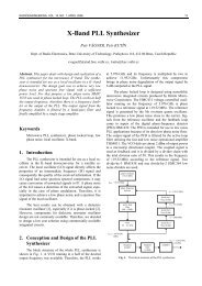
a)<br />
F<br />
b)<br />
F<br />
iterations<br />
iterations<br />
Fig. 3. Time responses <strong>of</strong> partial objective functions F f (matching),<br />
F g (gain), F p (polarization), and the global one F tot<br />
during the multi-objective optimization <strong>of</strong> the GPS antenna:<br />
a) genetic algorithm, b) particle swarm optimization.<br />
The described antenna is numerically analyzed by TDIE.<br />
Computed time responses <strong>of</strong> currents on discretization segments<br />
<strong>of</strong> the antenna are converted to frequency domain<br />
using fast Fourier transform. In frequency domain, criteria<br />
on matching, gain and polarization purity are formulated.<br />
The global objective function (3) is minimized using<br />
GA and PSO. Both the algorithms are allowed to perform<br />
100 iteration steps. Both the algorithms are run five times,<br />
and the best realization is considered in comparisons.
RADIOENGINEERING, VOL. 14, NO. 4, DECEMBER 2005 95<br />
b)<br />
a)<br />
deeper global minim (208.58 versus 227.28) compared to<br />
GA. Whereas the global objective function decreases monotonously,<br />
partial objective functions can both decrease<br />
and increase during the optimization. Partial objective functions<br />
should be <strong>of</strong> similar values to optimize successfully<br />
– hence the gain function F g and the polarization function<br />
F p should be enhanced by weighting coefficients up to the<br />
level <strong>of</strong> the matching function F f .<br />
a)<br />
Z<br />
[Ω]<br />
f<br />
[MHz]<br />
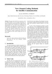
Fig. 4. The movement <strong>of</strong> individuals (agents) to the global optimum<br />
[F f , F g , F p ] = [ 0, 0, 0]: a) genetic algorithms, b) particle<br />
swarm optimization.<br />
b)<br />
Z<br />
[Ω]<br />
a)<br />
f<br />
[MHz]<br />
b)<br />
Fig. 5. Shape <strong>of</strong> the synthesized GPS antennas: a) the best individual<br />
by genetic algorithm, b) the best agent by particle<br />
swarm optimization.<br />
In Fig. 3, time responses <strong>of</strong> partial objective functions and<br />
the global one during the optimization <strong>of</strong> GPS antenna are<br />
depicted. Time response <strong>of</strong> PSO is smoother and reaches a<br />
Fig. 6. Impedance characteristics <strong>of</strong> the synthesized GPS antennas:<br />
a) genetic algorithm, b) particle swarm optimization.<br />
Fig. 4 shows the position <strong>of</strong> individuals (agents) in the coordinate<br />
system composed <strong>of</strong> partial objective functions F f ,<br />
F g and F p . The global optimum is identical with the point<br />
[0, 0, 0] in this coordinate system (the antenna perfectly<br />
meets requirements on matching, gain, and polarization<br />
purity). Agents <strong>of</strong> PSO are highly concentrated close to the<br />
global optimum; individuals <strong>of</strong> GA are more spread in the<br />
feasible space. Agents <strong>of</strong> PSO are closer to the global optimum<br />
compared to the individuals <strong>of</strong> GA.<br />
In Fig. 5, the synthesized monopoles (the best individual<br />
by GA and the best agent by PSO) are depicted.<br />
Impedance characteristic <strong>of</strong> the antennas are shown in<br />
Fig. 6. The GA antenna is accurately matched in both the<br />
bands, and moreover, the impedance characteristics are<br />
smooth without parasitic resonances. On the contrary, the<br />
PSO antenna is matched on slightly lower frequency in the<br />
lower band, and moreover, the frequency response <strong>of</strong> input<br />
impedance is corrupted by several resonances in between<br />
bands L2 and L1.
96 Z. LUKEŠ, Z. RAIDA, MULTI-OBJECTIVE OPTIMIZATION OF WIRE ANTENNAS: GENETIC ALGORITHMS VERSUS ...<br />
a)<br />
b)<br />
Fig. 7. Directivity pattern <strong>of</strong> the designed antenna in the band<br />
L1: a) genetic algorithm, b) particle swarm optimization.<br />
a)<br />
Fig. 9. Measured frequency response <strong>of</strong> the reflection coefficient<br />
<strong>of</strong> the designed antennas: genetic algorithm (top), particle<br />
swarm optimization (bottom).<br />
b)<br />
Measurements did not show any differences between the<br />
GA antenna and the PSO one from the viewpoint <strong>of</strong> impedance<br />
matching.<br />
Fig. 8. Directivity pattern <strong>of</strong> the designed antenna in the band<br />
L2: a) genetic algorithm, b) particle swarm optimization.<br />
Directivity patterns <strong>of</strong> the synthesized GPS antennas are<br />
depicted in Fig. 7 for the L1 band and in Fig 8 for the L2<br />
band. In both bands, the PSO antenna meets better the requirement<br />
on the constant gain for all directions.<br />
The matching criteria were also verified experimentally<br />
(see Fig. 9). The GA antenna exhibits the first minim<br />
<strong>of</strong> the reflection coefficient on 1248.5 MHz (the declination<br />
+2 %) and the second minim on 1521.5 MHz (the declination<br />
–4 %). Both minims are about –10 dB.<br />
The PSO antenna exhibits the first minim <strong>of</strong> the reflection<br />
coefficient on 1240.4 MHz (the declination +1 %)<br />
and the second minim on 1520.9 MHz (the declination –4<br />
per cent). Both minims are about –10 dB.<br />
5. Conclusions<br />
Our experience with the synthesis <strong>of</strong> wire antennas<br />
combining TDIE in the role <strong>of</strong> the computational tool plus<br />
GA and PSO as global optimizers can be concentrated into<br />
the following statements:<br />
• Both GA and PSO provide similar results <strong>of</strong> the synthesis.<br />
The synthesized antennas meet quite well the<br />
requirements. Weaknesses and advantages <strong>of</strong> solutions<br />
are both on the side <strong>of</strong> GA (better impedance<br />
characteristics, worse patterns) and PSO (better directivity<br />
patterns, worse characteristics).<br />
• S<strong>of</strong>tware implementation <strong>of</strong> PSO is simpler compared<br />
to GA: no coding and decoding <strong>of</strong> state variables is<br />
needed in case <strong>of</strong> PSO.<br />
• CPU-time demands <strong>of</strong> both PSO and GA are similar.<br />
The biggest portion <strong>of</strong> CPU time is consumed by evaluating<br />
directivity patterns (92 %). TDIE analysis is<br />
quite efficient (6 % <strong>of</strong> the total CPU time).<br />
The further development should be focused in the post-processing<br />
<strong>of</strong> the TDIE results to reduce the 92 per cent por-
RADIOENGINEERING, VOL. 14, NO. 4, DECEMBER 2005 97<br />
tion <strong>of</strong> the total CPU time consumed to the lower value.<br />
Formulating objective functions directly in the time domain<br />
might be one <strong>of</strong> possible solutions.<br />
Acknowledgements<br />
The research described in the paper was financially<br />
supported by the Czech Grant Agency under grants no.<br />
102/ 04/1079 and 102/03/H086, by the Czech Ministry <strong>of</strong><br />
Education under grant no. 2375/2005 and by the research<br />
program MSM 0021630513: Advanced Communication<br />
Systems and Technologies.<br />
References<br />
[1] RAO, S. M., WILTON, D. R. Transient scattering by conducting surfaces<br />
<strong>of</strong> arbitrary shape. IEEE Transactions on <strong>Antennas</strong> and Propagation.<br />
1991, vol. 39, no. 1, p. 56–61.<br />
[2] VECHINSKI, D. A., RAO, S. M. A stable procedure to calculate the<br />
transient scattering by conducting surfaces <strong>of</strong> arbitrary shape. IEEE<br />
Transactions on <strong>Antennas</strong> and Propagation. 1992, vol. 40, no. 6, p.<br />
661–665.<br />
[3] MANARA, G., MONORCHIO, A., REGGIANNINI, R. A spacetime<br />
discretization criterion for a stable time-marching solution <strong>of</strong><br />
the electric field integral equation. IEEE Transactions on <strong>Antennas</strong><br />
and Propagation. 1997, vol. 45, no. 3, p. 527–532.<br />
[4] BLUCK, M. J., WALKER, S. P. Time-domain BIE analysis <strong>of</strong> large<br />
three dimensional electromagnetic scattering problems. IEEE Transactions<br />
on <strong>Antennas</strong> and Propagation. 1997, vol. 45, no. 5, p. 894 to<br />
901.<br />
[5] SHANKER, B., ERGIN, A. A., AYGÜN, K., MICHIELSSEN, E.<br />
The plane wave time domain algorithm for the fast analysis <strong>of</strong> transient<br />
wave phenomena. IEEE <strong>Antennas</strong> and Propagation Magazine.<br />
1999, vol. 41, no. 4, p. 39–52.<br />
[6] HAUPT, R. L., An introduction to genetic algorithms for electromagnetics.<br />
IEEE <strong>Antennas</strong> and Propagation Magazine. 1995, vol. 37, no.<br />
2, p. 7–15.<br />
[7] WEILE, D. S., MICHIELSSEN, E. Genetic algorithm optimization<br />
applied to electromagnetics: a review. IEEE Transactions on <strong>Antennas</strong><br />
and Propagation. 1997, vol. 45, no. 3, p. 343–353.<br />
[8] JOHNSON, J. M., RAHMAT-SAMII, Y. Genetic algorithms in engineering<br />
electromagnetics. IEEE <strong>Antennas</strong> and Propagation Magazine.<br />
1997, vol. 39, no. 4, p. 7–21.<br />
[9] ALTMAN, Z., MITTRA, R., BOAG, A. new designs <strong>of</strong> ultra wideband<br />
communication antennas using a genetic algorithm. IEEE<br />
Transactions on <strong>Antennas</strong> and Propagation. 1997, vol. 45, no. 10, p.<br />
1494–1501.<br />
[10] JONES, E. A., JOINES, W. T. Design <strong>of</strong> Yagi-Uda antennas using<br />
genetic algorithms. IEEE Transactions on <strong>Antennas</strong> and Propagation.<br />
1997, vol. 45, no. 9, p. 1368–1392.<br />
[11] ZHIQIN Z., CHANG-HOI A., CARIN, L. Nonuniform frequency<br />
sampling with active learning: application to wide-band frequencydomain<br />
modeling and design. IEEE Transactions on <strong>Antennas</strong> and<br />
Propagation. 2005, vol. 53, no. 9, p. 3049–3057.<br />
[12] THORS, B., STEYSKAL, H., HOLTER, H. Broad-band fragmented<br />
aperture phased array element design using genetic algorithms. IEEE<br />
Transactions on <strong>Antennas</strong> and Propagation. 2005, vol. 53, no. 10, p.<br />
3280–3287.<br />
[13] KUWAHARA, Y. <strong>Multi</strong>objective optimization design <strong>of</strong> Yagi-Uda<br />
antenna. IEEE Transactions on <strong>Antennas</strong> and Propagation. 2005,<br />
vol. 53, no. 6, p. 1984–1992.<br />
[14] HOSUNG, C., ROGERS, R.L., HAO, L. Design <strong>of</strong> electrically small<br />
wire antennas using a Pareto genetic algorithm. IEEE Transactions<br />
on <strong>Antennas</strong> and Propagation. 2005, vol. 53, no. 3, p. 1038–1046.<br />
[15] CUI, S., MOHAN, A., WEILE, D. S. Pareto optimal design <strong>of</strong> absorbers<br />
using a parallel elitist nondominated sorting genetic algorithm<br />
and the finite element-boundary integral method. IEEE Transactions<br />
on <strong>Antennas</strong> and Propagation. 2005, vol. 53, no. 6, p. 2099–2107.<br />
[16] ROBINSON, J., RAHMAT-SAMII, Y. Particle swarm optimization<br />
in electromagnetics. IEEE Transactions on <strong>Antennas</strong> and Propagation.<br />
2004, vol. 52, no. 2, p. 397–407.<br />
[17] LIU, W. C. Design <strong>of</strong> a multiband CPW-fed monopole antenna using<br />
a particle swarm optimization approach. IEEE Transactions on <strong>Antennas</strong><br />
and Propagation. 2005, vol. 53, no. 10. p. 3273–3279.<br />
[18] BOERINGER, D.W., WERNER, D. H. Particle swarm optimization<br />
versus genetic algorithms for phased array synthesis. IEEE Transactions<br />
on <strong>Antennas</strong> and Propagation. 2004, vol. 52, no. 3, p. 771 to<br />
779.<br />
[19] LUKEŠ, Z., LÁČÍK, J., RAIDA, Z. Time domain wideband multiobjective<br />
genetic synthesis <strong>of</strong> wire antennas. In Proceeding <strong>of</strong> the<br />
13 th International Symposium on <strong>Antennas</strong> JINA 2004. Nice (France),<br />
2004, p. 366–369.<br />
[20] LUKEŠ, Z., ŠMÍD, P., RAIDA, Z. Broadband multi-objective synthesis<br />
<strong>of</strong> patch antennas. WSEAS Transactions on Computers. 2004,<br />
vol. 6, no. 3, p. 1863–1867.<br />
[21] LUKEŠ, Z., LÁČÍK, J., ŠMÍD, P., RAIDA, Z. <strong>Multi</strong>-objective synthesis<br />
<strong>of</strong> dual-band circularly polarized antennas by particle swarm<br />
optimization method. In Proceedings <strong>of</strong> the International Conference<br />
on Electromagnetics in Advanced Applications ICEAA 2005. Torino<br />
(Italy), 2005, p. 100–103.<br />
[22] RAIDA, Z., TKADLEC, R., FRANEK, O., MOTL, M., LÁČÍK, J.,<br />
LUKEŠ, Z., ŠKVOR, Z. Analýza mikrovlnných struktur v časové<br />
oblasti (Time-Domain Analysis <strong>of</strong> Microwave Structures). Brno:<br />
VUTIUM Publishing, 2003.<br />
[23] JORDAN, E. C., BALMAIN, K. G. Electromagnetic Waves and Radiating<br />
Systems. 2nd ed. Englewood Cliffs: Prentice Hall, 1968.<br />
About Authors...<br />
Zbyněk LUKEŠ graduated at the Faculty <strong>of</strong> Electrical<br />
Engineering and Communication (FEEC), Brno University<br />
<strong>of</strong> Technology (BUT), in 2002. Now, he has finished his<br />
dissertation at the Dept. <strong>of</strong> Radio Electronics, FEEC BUT.<br />
He is interested in the time-domain design <strong>of</strong> broadband<br />
planar and wire antennas.<br />
Zbyněk RAIDA – for biography, see p. 20 in this issue <strong>of</strong><br />
the <strong>Radioengineering</strong> journal.