Network Coding and Wireless Physical-layer ... - Jacobs University

More documents

Recommendations

Info

Chapter 6: Wireless Physical-layer Secret-key Generation (WPSG) in Relay Networks: Information Theoretic Limits, Key Extension, and Security Protocol 81 when there is only one or two paths, the correlation is significantly high. In [34], two rigorous metrics have been developed for quantifying the information theoretic limits of key generation in the scenario depicted in Fig. 6.3. Given the users have noisy channel estimates, which are denoted by ĥa, ĥa ′, ĥb, and ĥc, we refer to the maximum number of independent key bits that can be generated per channel observation as I K = I(h a ; h a ′), where I(x; y) denotes the mutual information between x and y. Likewise, the maximum number of independent key bits that can be generated and are secure from an eavesdropper is given by I SK = I(ĥa, ĥa ′|ĥb, ĥc) [76]. In [34], closed-form expressions for I K and I SK are derived for correlated complex Gaussian vector channels. The generated key bits that are not secure are called vulnerable key bits. The number of vulnerable key bits is therefore I V K = I K − I SK . To illustrate the key generation in Fig. 6.3, consider a simple scenario with scalar channels. Alice sends a pilot signal x to Bob, who derives the channel estimate ĥa of the channel h a from the received signal y b = h a x + n b , where n b denotes complex Gaussian noise on Bob’s side. After that, Bob sends x to Alice, who derives the estimate ĥa ′ of h a ′ in a similar manner. The number of available key bits I K per channel observation that can be generated by Alice and Bob is given by I K = I(ĥa; ĥa ′). If the time between Alice’s transmission and Bob’s is short and the same frequency band is used, we can assume reciprocity or h a = h a ′. Assuming further that h a is Rayleigh-distributed with a standard deviation of 0.5, we obtain a simulation result in Fig. 6.4 showing the relationship between I K and the signal-to-noise ratio, which is the ratio of the power of x to the Gaussian noise power at Bob and Alice. We also compute the result when the key is derived from the envelopes of channel parameters only, such that I K = I(|ĥa|; |ĥa ′|) [76]. 6.3 Possible Key Extensions In a general wireless network, the length of the key can be extended by having it generated from several transmission routes instead of only one. Although it is obvious that the total key length is the summation of the lengths from all paths, the key length from each path
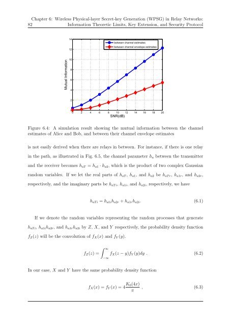
Chapter 6: Wireless Physical-layer Secret-key Generation (WPSG) in Relay Networks: 82 Information Theoretic Limits, Key Extension, and Security Protocol 14 12 between channel estimates between channel envelope estimates Mutual Information 10 8 6 4 2 0 0 2 4 6 8 10 12 14 16 18 20 SNR(dB) Figure 6.4: A simulation result showing the mutual information between the channel estimates of Alice and Bob, and between their channel envelope estimates is not easily derived when there are relays in between. For instance, if there is one relay in the path, as illustrated in Fig. 6.5, the channel parameter h a between the transmitter and the receiver becomes h aT = h a1 · h a2 , which is the product of two complex Gaussian random variables. If we let the real parts of h aT , h a1 , and h a2 be h aT r , h a1r , and h a2r , respectively, and the imaginary parts be h aT i , h a1i , and h a2i , respectively, we have h aT i = h a1i h a2r + h a1r h a2i . (6.1) If we denote the random variables representing the random processes that generate h aT i , h a1i h a2r , and h a1r h a2i by Z, X, and Y respectively, the probability density function f Z (z) will be the convolution of f X (x) and f Y (y). f Z (z) = ∫ ∞ −∞ f X (z − y)f Y (y)dy . (6.2) In our case, X and Y have the same probability density function f X (x) = f Y (x) = 4 K 0(4x) π , (6.3)
Page 1:
Network Coding and Wireless Physica
Page 4 and 5:
Abstract The general abstraction of
Page 6 and 7:
Contents Abstract i Abstract ii Dec
Page 8 and 9:
vi CONTENTS 5.4 Degree Distribution
Page 10 and 11:
List of Figures 2.1 A basic digital
Page 12 and 13:
x LIST OF FIGURES 5.11 Comparison o
Page 14 and 15:
Part I Motivation, Overview, and In
Page 16 and 17:
Chapter 1: Motivation and Overview
Page 18 and 19:
Chapter 2 Introduction to Digital C
Page 20 and 21:
Chapter 2: Introduction to Digital
Page 22 and 23:
Page 24 and 25:
Page 26 and 27:
Page 28 and 29:
Page 30 and 31:
Chapter 3: Introduction to Graphs a
Page 32 and 33:
Page 34 and 35:
Page 36 and 37:
Page 38 and 39:
Page 40 and 41:
Page 42 and 43:
Page 44 and 45: Chapter 3: Introduction to Graphs a
Page 46 and 47: 33 The emergence of scalable video
Page 48 and 49: Chapter 4: Unequal Erasure Protecti
Page 72 and 73: Chapter 5: Network Coding with LT C
Page 88 and 89: Part III Wireless Physical-layer Se
Page 90 and 91: Chapter 6 Wireless Physical-layer S
Page 92 and 93: Chapter 6: Wireless Physical-layer
Page 104 and 105: Chapter 7 Physical-layer Key Encodi
Page 106 and 107: Chapter 7: Physical-layer Key Encod
Page 124 and 125: Chapter 8: Summary, Conclusion, and
Page 132 and 133: Bibliography [1] 3GPP, “3GPP; Tec
Page 134 and 135: BIBLIOGRAPHY 121 [21] F.A. Hayek,
Page 136 and 137: BIBLIOGRAPHY 123 [43] M. Friedman a
Page 138 and 139: BIBLIOGRAPHY 125 [63] S. Jaggi, P.
Page 140: BIBLIOGRAPHY 127 [81] X. Sun, X. Wu
show all

Network Coding and Wireless Physical-layer ... - Jacobs University

Create successful ePaper yourself

Delete template?

Save as template?