Quality and Reliability Methods - SAS

Version 10 

Quality and Reliability 

Methods 

“The real voyage of discovery consists not in seeking new 

landscapes, but in having new eyes.” 

Marcel Proust 

JMP, A Business Unit of SAS 

SAS Campus Drive 

Cary, NC 27513 10.0.2

The correct bibliographic citation for this manual is as follows: SAS Institute Inc. 2012. JMP ® 10 

Quality and Reliability Methods. Cary, NC: SAS Institute Inc. 

JMP ® 10 Quality and Reliability Methods 

Copyright © 2012, SAS Institute Inc., Cary, NC, USA 

ISBN 978-1-61290-199-2 

All rights reserved. Produced in the United States of America. 

For a hard-copy book: No part of this publication may be reproduced, stored in a retrieval system, or 

transmitted, in any form or by any means, electronic, mechanical, photocopying, or otherwise, without 

the prior written permission of the publisher, SAS Institute Inc. 

For a Web download or e-book: Your use of this publication shall be governed by the terms established 

by the vendor at the time you acquire this publication. 

The scanning, uploading, and distribution of this book via the Internet or any other means without the 

permission of the publisher is illegal and punishable by law. Please purchase only authorized electronic 

editions and do not participate in or encourage electronic piracy of copyrighted materials. Your support 

of others’ rights is appreciated. 

U.S. Government Restricted Rights Notice: Use, duplication, or disclosure of this software and related 

documentation by the U.S. government is subject to the Agreement with SAS Institute and the 

restrictions set forth in FAR 52.227-19, Commercial Computer Software-Restricted Rights (June 1987). 

SAS Institute Inc., SAS Campus Drive, Cary, North Carolina 27513. 

1st printing, March 2012 

2nd printing, July 2012 

3rd printing, November 2012 

SAS ® Publishing provides a complete selection of books and electronic products to help customers use 

SAS software to its fullest potential. For more information about our e-books, e-learning products, CDs, 

and hard-copy books, visit the SAS Publishing Web site at support.sas.com/publishing or call 

1-800-727-3228. 

SAS ® and all other SAS Institute Inc. product or service names are registered trademarks or trademarks 

of SAS Institute Inc. in the USA and other countries. ® indicates USA registration. 

Other brand and product names are registered trademarks or trademarks of their respective companies. 

Technology License Notices 

Scintilla is Copyright © 1998-2003 by Neil Hodgson . NEIL HODGSON DISCLAIMS 

ALL WARRANTIES WITH REGARD TO THIS SOFTWARE, INCLUDING ALL IMPLIED WARRANTIES OF 

MERCHANTABILITY AND FITNESS, IN NO EVENT SHALL NEIL HODGSON BE LIABLE FOR ANY SPECIAL,

INDIRECT OR CONSEQUENTIAL DAMAGES OR ANY DAMAGES WHATSOEVER RESULTING FROM LOSS OF 

USE, DATA OR PROFITS, WHETHER IN AN ACTION OF CONTRACT, NEGLIGENCE OR OTHER TORTIOUS 

ACTION, ARISING OUT OF OR IN CONNECTION WITH THE USE OR PERFORMANCE OF THIS SOFTWARE. 

XRender is Copyright © 2002 Keith Packard. KEITH PACKARD DISCLAIMS ALL WARRANTIES WITH 

REGARD TO THIS SOFTWARE, INCLUDING ALL IMPLIED WARRANTIES OF MERCHANTABILITY AND 

FITNESS, IN NO EVENT SHALL KEITH PACKARD BE LIABLE FOR ANY SPECIAL, INDIRECT OR 

CONSEQUENTIAL DAMAGES OR ANY DAMAGES WHATSOEVER RESULTING FROM LOSS OF USE, DATA OR 

PROFITS, WHETHER IN AN ACTION OF CONTRACT, NEGLIGENCE OR OTHER TORTIOUS ACTION, 

ARISING OUT OF OR IN CONNECTION WITH THE USE OR PERFORMANCE OF THIS SOFTWARE. 

ImageMagick software is Copyright © 1999-2011, ImageMagick Studio LLC, a non-profit organization 

dedicated to making software imaging solutions freely available. 

bzlib software is Copyright © 1991-2009, Thomas G. Lane, Guido Vollbeding. All rights reserved. 

FreeType software is Copyright © 1996-2002, The FreeType Project (www.freetype.org). All rights 

reserved. 

Get the Most from JMP ® 

Whether you are a first-time or a long-time user, there is always something to learn about JMP. 

Visit JMP.com to find the following: 

• live and recorded Webcasts about how to get started with JMP 

• video demos and Webcasts of new features and advanced techniques 

• schedules for seminars being held in your area 

• success stories showing how others use JMP 

• a blog with tips, tricks, and stories from JMP staff 

• a forum to discuss JMP with other users 

http://www.jmp.com/getstarted/

Contents 

JMP Quality and Reliability Methods 

1 Learn about JMP 

Documentation and Additional Resources . . . . . . . . . . . . . . . . . . . . . . . . . . . . . . . . . . . . . . . 15 

Book Conventions . . . . . . . . . . . . . . . . . . . . . . . . . . . . . . . . . . . . . . . . . . . . . . . . . . . . . . . . . . . . . . . . 17 

JMP Documentation . . . . . . . . . . . . . . . . . . . . . . . . . . . . . . . . . . . . . . . . . . . . . . . . . . . . . . . . . . . . . . 17 

JMP Documentation Suite . . . . . . . . . . . . . . . . . . . . . . . . . . . . . . . . . . . . . . . . . . . . . . . . . . . . . . . 18 

JMP Help . . . . . . . . . . . . . . . . . . . . . . . . . . . . . . . . . . . . . . . . . . . . . . . . . . . . . . . . . . . . . . . . . . . . 21 

JMP Books by Users . . . . . . . . . . . . . . . . . . . . . . . . . . . . . . . . . . . . . . . . . . . . . . . . . . . . . . . . . . . . 21 

JMPer Cable . . . . . . . . . . . . . . . . . . . . . . . . . . . . . . . . . . . . . . . . . . . . . . . . . . . . . . . . . . . . . . . . . . 21 

Additional Resources for Learning JMP . . . . . . . . . . . . . . . . . . . . . . . . . . . . . . . . . . . . . . . . . . . . . . . . 21 

Tutorials . . . . . . . . . . . . . . . . . . . . . . . . . . . . . . . . . . . . . . . . . . . . . . . . . . . . . . . . . . . . . . . . . . . . . 21 

The JMP Starter Window . . . . . . . . . . . . . . . . . . . . . . . . . . . . . . . . . . . . . . . . . . . . . . . . . . . . . . . 22 

Sample Data Tables . . . . . . . . . . . . . . . . . . . . . . . . . . . . . . . . . . . . . . . . . . . . . . . . . . . . . . . . . . . . 22 

Learn about Statistical and JSL Terms . . . . . . . . . . . . . . . . . . . . . . . . . . . . . . . . . . . . . . . . . . . . . . 22 

Learn JMP Tips and Tricks . . . . . . . . . . . . . . . . . . . . . . . . . . . . . . . . . . . . . . . . . . . . . . . . . . . . . . . 22 

Tooltips . . . . . . . . . . . . . . . . . . . . . . . . . . . . . . . . . . . . . . . . . . . . . . . . . . . . . . . . . . . . . . . . . . . . . 23 

Access Resources on the Web . . . . . . . . . . . . . . . . . . . . . . . . . . . . . . . . . . . . . . . . . . . . . . . . . . . . . 23 

2 Statistical Control Charts 

The Control Chart Platform . . . . . . . . . . . . . . . . . . . . . . . . . . . . . . . . . . . . . . . . . . . . . . . . . . . . . 25 

Statistical Quality Control with Control Charts . . . . . . . . . . . . . . . . . . . . . . . . . . . . . . . . . . . . . . . . . . 27 

The Control Chart Launch Dialog . . . . . . . . . . . . . . . . . . . . . . . . . . . . . . . . . . . . . . . . . . . . . . . . . . . . 27 

Process Information . . . . . . . . . . . . . . . . . . . . . . . . . . . . . . . . . . . . . . . . . . . . . . . . . . . . . . . . . . . . 28 

Chart Type Information . . . . . . . . . . . . . . . . . . . . . . . . . . . . . . . . . . . . . . . . . . . . . . . . . . . . . . . . . 31 

Parameters . . . . . . . . . . . . . . . . . . . . . . . . . . . . . . . . . . . . . . . . . . . . . . . . . . . . . . . . . . . . . . . . . . . 32 

Using Specified Statistics . . . . . . . . . . . . . . . . . . . . . . . . . . . . . . . . . . . . . . . . . . . . . . . . . . . . . . . . 33 

Tailoring the Horizontal Axis . . . . . . . . . . . . . . . . . . . . . . . . . . . . . . . . . . . . . . . . . . . . . . . . . . . . . . . . 34 

Display Options . . . . . . . . . . . . . . . . . . . . . . . . . . . . . . . . . . . . . . . . . . . . . . . . . . . . . . . . . . . . . . . . . . 34 

Single Chart Options . . . . . . . . . . . . . . . . . . . . . . . . . . . . . . . . . . . . . . . . . . . . . . . . . . . . . . . . . . . 34 

Window Options . . . . . . . . . . . . . . . . . . . . . . . . . . . . . . . . . . . . . . . . . . . . . . . . . . . . . . . . . . . . . . 37 

Tests for Special Causes . . . . . . . . . . . . . . . . . . . . . . . . . . . . . . . . . . . . . . . . . . . . . . . . . . . . . . . . . . . . 39

6 

Nelson Rules . . . . . . . . . . . . . . . . . . . . . . . . . . . . . . . . . . . . . . . . . . . . . . . . . . . . . . . . . . . . . . . . . . 39 

Westgard Rules . . . . . . . . . . . . . . . . . . . . . . . . . . . . . . . . . . . . . . . . . . . . . . . . . . . . . . . . . . . . . . . 42 

Running Alarm Scripts . . . . . . . . . . . . . . . . . . . . . . . . . . . . . . . . . . . . . . . . . . . . . . . . . . . . . . . . . . . . 44 

Saving and Retrieving Limits . . . . . . . . . . . . . . . . . . . . . . . . . . . . . . . . . . . . . . . . . . . . . . . . . . . . . . . . . 45 

Real-Time Data Capture . . . . . . . . . . . . . . . . . . . . . . . . . . . . . . . . . . . . . . . . . . . . . . . . . . . . . . . . . . . 49 

The Open Datafeed Command . . . . . . . . . . . . . . . . . . . . . . . . . . . . . . . . . . . . . . . . . . . . . . . . . . . 49 

Commands for Data Feed . . . . . . . . . . . . . . . . . . . . . . . . . . . . . . . . . . . . . . . . . . . . . . . . . . . . . . . 49 

Operation . . . . . . . . . . . . . . . . . . . . . . . . . . . . . . . . . . . . . . . . . . . . . . . . . . . . . . . . . . . . . . . . . . . 50 

Setting Up a Script to Start a New Data Table . . . . . . . . . . . . . . . . . . . . . . . . . . . . . . . . . . . . . . . . 50 

Setting Up a Script in a Data Table . . . . . . . . . . . . . . . . . . . . . . . . . . . . . . . . . . . . . . . . . . . . . . . . . 51 

Excluded, Hidden, and Deleted Samples . . . . . . . . . . . . . . . . . . . . . . . . . . . . . . . . . . . . . . . . . . . . . . . . 51 

3 Introduction to Control Charts 

Control Chart Platforms . . . . . . . . . . . . . . . . . . . . . . . . . . . . . . . . . . . . . . . . . . . . . . . . . . . . . . . . 53 

What is a Control Chart? . . . . . . . . . . . . . . . . . . . . . . . . . . . . . . . . . . . . . . . . . . . . . . . . . . . . . . . . . . . 55 

Parts of a Control Chart . . . . . . . . . . . . . . . . . . . . . . . . . . . . . . . . . . . . . . . . . . . . . . . . . . . . . . . . . . . . 55 

Control Charts in JMP . . . . . . . . . . . . . . . . . . . . . . . . . . . . . . . . . . . . . . . . . . . . . . . . . . . . . . . . . . . . . 56 

Types and Availability on Chart Charts . . . . . . . . . . . . . . . . . . . . . . . . . . . . . . . . . . . . . . . . . . . . . . . . . 57 

4 Interactive Control Charts 

The Control Chart Builder Platform . . . . . . . . . . . . . . . . . . . . . . . . . . . . . . . . . . . . . . . . . . . . . . 59 

Overview of Control Chart Builder . . . . . . . . . . . . . . . . . . . . . . . . . . . . . . . . . . . . . . . . . . . . . . . . . . . . 61 

Example Using Control Chart Builder . . . . . . . . . . . . . . . . . . . . . . . . . . . . . . . . . . . . . . . . . . . . . . . . . 61 

Launch Control Chart Builder . . . . . . . . . . . . . . . . . . . . . . . . . . . . . . . . . . . . . . . . . . . . . . . . . . . . . . . 63 

Control Chart Builder Options . . . . . . . . . . . . . . . . . . . . . . . . . . . . . . . . . . . . . . . . . . . . . . . . . . . . . . 64 

Additional Example of Control Chart Builder . . . . . . . . . . . . . . . . . . . . . . . . . . . . . . . . . . . . . . . . . . . 67 

5 Shewhart Control Charts 

Variables and Attribute Control Charts . . . . . . . . . . . . . . . . . . . . . . . . . . . . . . . . . . . . . . . . . . 69 

Shewhart Control Charts for Variables . . . . . . . . . . . . . . . . . . . . . . . . . . . . . . . . . . . . . . . . . . . . . . . . . 71 

XBar-, R-, and S- Charts . . . . . . . . . . . . . . . . . . . . . . . . . . . . . . . . . . . . . . . . . . . . . . . . . . . . . . . . . 71 

Run Charts . . . . . . . . . . . . . . . . . . . . . . . . . . . . . . . . . . . . . . . . . . . . . . . . . . . . . . . . . . . . . . . . . . 76 

Individual Measurement Charts . . . . . . . . . . . . . . . . . . . . . . . . . . . . . . . . . . . . . . . . . . . . . . . . . . 76 

Presummarize Charts . . . . . . . . . . . . . . . . . . . . . . . . . . . . . . . . . . . . . . . . . . . . . . . . . . . . . . . . . . . 79 

Moving Average Charts . . . . . . . . . . . . . . . . . . . . . . . . . . . . . . . . . . . . . . . . . . . . . . . . . . . . . . . . . . . . . 81 

Uniformly Weighted Moving Average (UWMA) Charts . . . . . . . . . . . . . . . . . . . . . . . . . . . . . . . . . 81

7 

Exponentially Weighted Moving Average (EWMA) Charts . . . . . . . . . . . . . . . . . . . . . . . . . . . . . . 83 

Shewhart Control Charts for Attributes . . . . . . . . . . . . . . . . . . . . . . . . . . . . . . . . . . . . . . . . . . . . . . . . 85 

P- and NP-Charts . . . . . . . . . . . . . . . . . . . . . . . . . . . . . . . . . . . . . . . . . . . . . . . . . . . . . . . . . . . . . 86 

U-Charts . . . . . . . . . . . . . . . . . . . . . . . . . . . . . . . . . . . . . . . . . . . . . . . . . . . . . . . . . . . . . . . . . . . . 88 

C-Charts . . . . . . . . . . . . . . . . . . . . . . . . . . . . . . . . . . . . . . . . . . . . . . . . . . . . . . . . . . . . . . . . . . . . 89 

Levey-Jennings Charts . . . . . . . . . . . . . . . . . . . . . . . . . . . . . . . . . . . . . . . . . . . . . . . . . . . . . . . . . . 91 

Phases . . . . . . . . . . . . . . . . . . . . . . . . . . . . . . . . . . . . . . . . . . . . . . . . . . . . . . . . . . . . . . . . . . . . . . . . . 91 

Example . . . . . . . . . . . . . . . . . . . . . . . . . . . . . . . . . . . . . . . . . . . . . . . . . . . . . . . . . . . . . . . . . . . . . 92 

JSL Phase Level Limits . . . . . . . . . . . . . . . . . . . . . . . . . . . . . . . . . . . . . . . . . . . . . . . . . . . . . . . . . . 93 

6 Cumulative Sum Control Charts 

CUSUM Charts . . . . . . . . . . . . . . . . . . . . . . . . . . . . . . . . . . . . . . . . . . . . . . . . . . . . . . . . . . . . . . . . 95 

Cumulative Sum (Cusum) Charts . . . . . . . . . . . . . . . . . . . . . . . . . . . . . . . . . . . . . . . . . . . . . . . . . . . . 97 

Launch Options for Cusum Charts . . . . . . . . . . . . . . . . . . . . . . . . . . . . . . . . . . . . . . . . . . . . . . . . 98 

Cusum Chart Options . . . . . . . . . . . . . . . . . . . . . . . . . . . . . . . . . . . . . . . . . . . . . . . . . . . . . . . . . . 99 

Formulas for CUSUM Charts . . . . . . . . . . . . . . . . . . . . . . . . . . . . . . . . . . . . . . . . . . . . . . . . . . . . . . 104 

Notation . . . . . . . . . . . . . . . . . . . . . . . . . . . . . . . . . . . . . . . . . . . . . . . . . . . . . . . . . . . . . . . . . . . 104 

One-Sided CUSUM Charts . . . . . . . . . . . . . . . . . . . . . . . . . . . . . . . . . . . . . . . . . . . . . . . . . . . . . 104 

Two-Sided Cusum Schemes . . . . . . . . . . . . . . . . . . . . . . . . . . . . . . . . . . . . . . . . . . . . . . . . . . . . . 106 

7 Multivariate Control Charts 

Quality Control for Multivariate Data . . . . . . . . . . . . . . . . . . . . . . . . . . . . . . . . . . . . . . . . . . . 107 

Launch the Platform . . . . . . . . . . . . . . . . . . . . . . . . . . . . . . . . . . . . . . . . . . . . . . . . . . . . . . . . . . . . . 109 

Control Chart Usage . . . . . . . . . . . . . . . . . . . . . . . . . . . . . . . . . . . . . . . . . . . . . . . . . . . . . . . . . . . . . 109 

Phase 1—Obtaining Targets . . . . . . . . . . . . . . . . . . . . . . . . . . . . . . . . . . . . . . . . . . . . . . . . . . . . . 109 

Phase 2—Monitoring the Process . . . . . . . . . . . . . . . . . . . . . . . . . . . . . . . . . . . . . . . . . . . . . . . . . . 110 

Monitoring a Grouped Process . . . . . . . . . . . . . . . . . . . . . . . . . . . . . . . . . . . . . . . . . . . . . . . . . . . . 111 

Change Point Detection . . . . . . . . . . . . . . . . . . . . . . . . . . . . . . . . . . . . . . . . . . . . . . . . . . . . . . . . . . . . 113 

Method . . . . . . . . . . . . . . . . . . . . . . . . . . . . . . . . . . . . . . . . . . . . . . . . . . . . . . . . . . . . . . . . . . . . . 114 

Example . . . . . . . . . . . . . . . . . . . . . . . . . . . . . . . . . . . . . . . . . . . . . . . . . . . . . . . . . . . . . . . . . . . . . 114 

Platform Options . . . . . . . . . . . . . . . . . . . . . . . . . . . . . . . . . . . . . . . . . . . . . . . . . . . . . . . . . . . . . . . . . 115 

Statistical Details . . . . . . . . . . . . . . . . . . . . . . . . . . . . . . . . . . . . . . . . . . . . . . . . . . . . . . . . . . . . . . . . . 116 

Ungrouped Data . . . . . . . . . . . . . . . . . . . . . . . . . . . . . . . . . . . . . . . . . . . . . . . . . . . . . . . . . . . . . . 116 

Grouped Data . . . . . . . . . . . . . . . . . . . . . . . . . . . . . . . . . . . . . . . . . . . . . . . . . . . . . . . . . . . . . . . . 117 

Additivity . . . . . . . . . . . . . . . . . . . . . . . . . . . . . . . . . . . . . . . . . . . . . . . . . . . . . . . . . . . . . . . . . . . . 118 

Change Point Detection . . . . . . . . . . . . . . . . . . . . . . . . . . . . . . . . . . . . . . . . . . . . . . . . . . . . . . . . . 118

8 

8 Assess Measurement Systems 

The Measurement Systems Analysis Platform . . . . . . . . . . . . . . . . . . . . . . . . . . . . . . . . . . . 121 

Overview of Measurement Systems Analysis . . . . . . . . . . . . . . . . . . . . . . . . . . . . . . . . . . . . . . . . . . . . 123 

Example of Measurement Systems Analysis . . . . . . . . . . . . . . . . . . . . . . . . . . . . . . . . . . . . . . . . . . . . . 123 

Launch the Measurement Systems Analysis Platform . . . . . . . . . . . . . . . . . . . . . . . . . . . . . . . . . . . . . . 126 

Measurement Systems Analysis Platform Options . . . . . . . . . . . . . . . . . . . . . . . . . . . . . . . . . . . . . . . . 127 

Average Chart . . . . . . . . . . . . . . . . . . . . . . . . . . . . . . . . . . . . . . . . . . . . . . . . . . . . . . . . . . . . . . . . 129 

Range Chart or Standard Deviation Chart . . . . . . . . . . . . . . . . . . . . . . . . . . . . . . . . . . . . . . . . . . . 129 

EMP Results . . . . . . . . . . . . . . . . . . . . . . . . . . . . . . . . . . . . . . . . . . . . . . . . . . . . . . . . . . . . . . . . . 129 

Effective Resolution . . . . . . . . . . . . . . . . . . . . . . . . . . . . . . . . . . . . . . . . . . . . . . . . . . . . . . . . . . . . 131 

Shift Detection Profiler . . . . . . . . . . . . . . . . . . . . . . . . . . . . . . . . . . . . . . . . . . . . . . . . . . . . . . . . . 132 

Bias Comparison . . . . . . . . . . . . . . . . . . . . . . . . . . . . . . . . . . . . . . . . . . . . . . . . . . . . . . . . . . . . . . 132 

Test-Retest Error Comparison . . . . . . . . . . . . . . . . . . . . . . . . . . . . . . . . . . . . . . . . . . . . . . . . . . . . 133 

Additional Example of Measurement Systems Analysis . . . . . . . . . . . . . . . . . . . . . . . . . . . . . . . . . . . . 133 

Statistical Details for Measurement Systems Analysis . . . . . . . . . . . . . . . . . . . . . . . . . . . . . . . . . . . . . . 139 

9 Capability Analyses 

The Capability Platform . . . . . . . . . . . . . . . . . . . . . . . . . . . . . . . . . . . . . . . . . . . . . . . . . . . . . . . . 141 

Launch the Platform . . . . . . . . . . . . . . . . . . . . . . . . . . . . . . . . . . . . . . . . . . . . . . . . . . . . . . . . . . . . . . 143 

Entering Limits . . . . . . . . . . . . . . . . . . . . . . . . . . . . . . . . . . . . . . . . . . . . . . . . . . . . . . . . . . . . . . . 143 

Capability Plots and Options . . . . . . . . . . . . . . . . . . . . . . . . . . . . . . . . . . . . . . . . . . . . . . . . . . . . . . . 145 

Goal Plot . . . . . . . . . . . . . . . . . . . . . . . . . . . . . . . . . . . . . . . . . . . . . . . . . . . . . . . . . . . . . . . . . . . . 145 

Capability Box Plots . . . . . . . . . . . . . . . . . . . . . . . . . . . . . . . . . . . . . . . . . . . . . . . . . . . . . . . . . . . 146 

Normalized Box Plots . . . . . . . . . . . . . . . . . . . . . . . . . . . . . . . . . . . . . . . . . . . . . . . . . . . . . . . . . . 148 

Individual Detail Reports . . . . . . . . . . . . . . . . . . . . . . . . . . . . . . . . . . . . . . . . . . . . . . . . . . . . . . . 149 

Make Summary Table . . . . . . . . . . . . . . . . . . . . . . . . . . . . . . . . . . . . . . . . . . . . . . . . . . . . . . . . . . 149 

Capability Indices Report . . . . . . . . . . . . . . . . . . . . . . . . . . . . . . . . . . . . . . . . . . . . . . . . . . . . . . . 150 

10 Variability Charts 

Variability Chart and Gauge R&R Analysis . . . . . . . . . . . . . . . . . . . . . . . . . . . . . . . . . . . . . . . 151 

Variability Charts . . . . . . . . . . . . . . . . . . . . . . . . . . . . . . . . . . . . . . . . . . . . . . . . . . . . . . . . . . . . . . . . 153 

Launch the Variability Platform . . . . . . . . . . . . . . . . . . . . . . . . . . . . . . . . . . . . . . . . . . . . . . . . . . . 153 

Variability Chart . . . . . . . . . . . . . . . . . . . . . . . . . . . . . . . . . . . . . . . . . . . . . . . . . . . . . . . . . . . . . . 154 

Variability Platform Options . . . . . . . . . . . . . . . . . . . . . . . . . . . . . . . . . . . . . . . . . . . . . . . . . . . . . 155 

Heterogeneity of Variance Tests . . . . . . . . . . . . . . . . . . . . . . . . . . . . . . . . . . . . . . . . . . . . . . . . . . . 158 

Variance Components . . . . . . . . . . . . . . . . . . . . . . . . . . . . . . . . . . . . . . . . . . . . . . . . . . . . . . . . . . . . . 160 

Variance Component Method . . . . . . . . . . . . . . . . . . . . . . . . . . . . . . . . . . . . . . . . . . . . . . . . . . . . 161

9 

R&R Measurement Systems . . . . . . . . . . . . . . . . . . . . . . . . . . . . . . . . . . . . . . . . . . . . . . . . . . . . . . . . 163 

Gauge R&R Variability Report . . . . . . . . . . . . . . . . . . . . . . . . . . . . . . . . . . . . . . . . . . . . . . . . . . 164 

Misclassification Probabilities . . . . . . . . . . . . . . . . . . . . . . . . . . . . . . . . . . . . . . . . . . . . . . . . . . . . 166 

Bias . . . . . . . . . . . . . . . . . . . . . . . . . . . . . . . . . . . . . . . . . . . . . . . . . . . . . . . . . . . . . . . . . . . . . . . 166 

Linearity Study . . . . . . . . . . . . . . . . . . . . . . . . . . . . . . . . . . . . . . . . . . . . . . . . . . . . . . . . . . . . . . . 168 

Discrimination Ratio Report . . . . . . . . . . . . . . . . . . . . . . . . . . . . . . . . . . . . . . . . . . . . . . . . . . . . . . . 169 

Attribute Gauge Charts . . . . . . . . . . . . . . . . . . . . . . . . . . . . . . . . . . . . . . . . . . . . . . . . . . . . . . . . . . . 169 

Data Organization . . . . . . . . . . . . . . . . . . . . . . . . . . . . . . . . . . . . . . . . . . . . . . . . . . . . . . . . . . . . 170 

Launching the Platform . . . . . . . . . . . . . . . . . . . . . . . . . . . . . . . . . . . . . . . . . . . . . . . . . . . . . . . . 170 

Platform Options . . . . . . . . . . . . . . . . . . . . . . . . . . . . . . . . . . . . . . . . . . . . . . . . . . . . . . . . . . . . . . 171 

Attribute Gauge Plots . . . . . . . . . . . . . . . . . . . . . . . . . . . . . . . . . . . . . . . . . . . . . . . . . . . . . . . . . . . 171 

Agreement . . . . . . . . . . . . . . . . . . . . . . . . . . . . . . . . . . . . . . . . . . . . . . . . . . . . . . . . . . . . . . . . . . 173 

Effectiveness Report . . . . . . . . . . . . . . . . . . . . . . . . . . . . . . . . . . . . . . . . . . . . . . . . . . . . . . . . . . . 176 

11 Pareto Plots 

The Pareto Plot Platform . . . . . . . . . . . . . . . . . . . . . . . . . . . . . . . . . . . . . . . . . . . . . . . . . . . . . . 179 

Pareto Plots . . . . . . . . . . . . . . . . . . . . . . . . . . . . . . . . . . . . . . . . . . . . . . . . . . . . . . . . . . . . . . . . . . . . . 181 

Assigning Variable Roles . . . . . . . . . . . . . . . . . . . . . . . . . . . . . . . . . . . . . . . . . . . . . . . . . . . . . . . . . 181 

Pareto Plot Platform Commands . . . . . . . . . . . . . . . . . . . . . . . . . . . . . . . . . . . . . . . . . . . . . . . . . . 183 

Options for Bars . . . . . . . . . . . . . . . . . . . . . . . . . . . . . . . . . . . . . . . . . . . . . . . . . . . . . . . . . . . . . . . 185 

Launch Dialog Options . . . . . . . . . . . . . . . . . . . . . . . . . . . . . . . . . . . . . . . . . . . . . . . . . . . . . . . . . . . 187 

Threshold of Combined Causes . . . . . . . . . . . . . . . . . . . . . . . . . . . . . . . . . . . . . . . . . . . . . . . . . . 187 

One-Way Comparative Pareto Plot . . . . . . . . . . . . . . . . . . . . . . . . . . . . . . . . . . . . . . . . . . . . . . . . . . 188 

Two-Way Comparative Pareto Plot . . . . . . . . . . . . . . . . . . . . . . . . . . . . . . . . . . . . . . . . . . . . . . . . . . . 190 

Defect Per Unit Analysis . . . . . . . . . . . . . . . . . . . . . . . . . . . . . . . . . . . . . . . . . . . . . . . . . . . . . . . . . . . 192 

Using Number of Defects as Sample Size . . . . . . . . . . . . . . . . . . . . . . . . . . . . . . . . . . . . . . . . . . . 192 

Using a Constant Sample Size Across Groups . . . . . . . . . . . . . . . . . . . . . . . . . . . . . . . . . . . . . . . . 192 

Using a Non-Constant Sample Size Across Groups . . . . . . . . . . . . . . . . . . . . . . . . . . . . . . . . . . . . 194 

12 Ishikawa Diagrams 

The Diagram Platform . . . . . . . . . . . . . . . . . . . . . . . . . . . . . . . . . . . . . . . . . . . . . . . . . . . . . . . . . 197 

Preparing the Data for Diagramming . . . . . . . . . . . . . . . . . . . . . . . . . . . . . . . . . . . . . . . . . . . . . . . . . 199 

Chart Types . . . . . . . . . . . . . . . . . . . . . . . . . . . . . . . . . . . . . . . . . . . . . . . . . . . . . . . . . . . . . . . . . . . . 200 

Building a Chart Interactively . . . . . . . . . . . . . . . . . . . . . . . . . . . . . . . . . . . . . . . . . . . . . . . . . . . . . . 201 

Text Menu . . . . . . . . . . . . . . . . . . . . . . . . . . . . . . . . . . . . . . . . . . . . . . . . . . . . . . . . . . . . . . . . . . 201 

Insert Menu . . . . . . . . . . . . . . . . . . . . . . . . . . . . . . . . . . . . . . . . . . . . . . . . . . . . . . . . . . . . . . . . . 202 

Move Menu . . . . . . . . . . . . . . . . . . . . . . . . . . . . . . . . . . . . . . . . . . . . . . . . . . . . . . . . . . . . . . . . . 203

10 

Other Menu Options . . . . . . . . . . . . . . . . . . . . . . . . . . . . . . . . . . . . . . . . . . . . . . . . . . . . . . . . . . 205 

Drag and Drop . . . . . . . . . . . . . . . . . . . . . . . . . . . . . . . . . . . . . . . . . . . . . . . . . . . . . . . . . . . . . . . 205 

13 Lifetime Distribution 

Using the Life Distribution Platform . . . . . . . . . . . . . . . . . . . . . . . . . . . . . . . . . . . . . . . . . . . . 207 

Overview of Life Distribution Analysis . . . . . . . . . . . . . . . . . . . . . . . . . . . . . . . . . . . . . . . . . . . . . . . 209 

Example of Life Distribution Analysis . . . . . . . . . . . . . . . . . . . . . . . . . . . . . . . . . . . . . . . . . . . . . . . . 209 

Launch the Life Distribution Platform . . . . . . . . . . . . . . . . . . . . . . . . . . . . . . . . . . . . . . . . . . . . . . . . 212 

The Life Distribution Report Window . . . . . . . . . . . . . . . . . . . . . . . . . . . . . . . . . . . . . . . . . . . . . . . . 213 

Event Plot . . . . . . . . . . . . . . . . . . . . . . . . . . . . . . . . . . . . . . . . . . . . . . . . . . . . . . . . . . . . . . . . . . . 213 

Compare Distributions Report . . . . . . . . . . . . . . . . . . . . . . . . . . . . . . . . . . . . . . . . . . . . . . . . . . . 215 

Statistics Report . . . . . . . . . . . . . . . . . . . . . . . . . . . . . . . . . . . . . . . . . . . . . . . . . . . . . . . . . . . . . . . 216 

Competing Cause Report . . . . . . . . . . . . . . . . . . . . . . . . . . . . . . . . . . . . . . . . . . . . . . . . . . . . . . . 218 

Life Distribution Platform Options . . . . . . . . . . . . . . . . . . . . . . . . . . . . . . . . . . . . . . . . . . . . . . . . . . 220 

Additional Examples of the Life Distribution Platform . . . . . . . . . . . . . . . . . . . . . . . . . . . . . . . . . . . . 221 

Omit Competing Causes . . . . . . . . . . . . . . . . . . . . . . . . . . . . . . . . . . . . . . . . . . . . . . . . . . . . . . . . 221 

Change the Scale . . . . . . . . . . . . . . . . . . . . . . . . . . . . . . . . . . . . . . . . . . . . . . . . . . . . . . . . . . . . . . 223 

Statistical Details . . . . . . . . . . . . . . . . . . . . . . . . . . . . . . . . . . . . . . . . . . . . . . . . . . . . . . . . . . . . . . . . . 225 

Nonparametric Fit . . . . . . . . . . . . . . . . . . . . . . . . . . . . . . . . . . . . . . . . . . . . . . . . . . . . . . . . . . . . . 226 

Parametric Distributions . . . . . . . . . . . . . . . . . . . . . . . . . . . . . . . . . . . . . . . . . . . . . . . . . . . . . . . . 226 

14 Lifetime Distribution II 

The Fit Life by X Platform . . . . . . . . . . . . . . . . . . . . . . . . . . . . . . . . . . . . . . . . . . . . . . . . . . . . . . 237 

Introduction to Accelerated Test Models . . . . . . . . . . . . . . . . . . . . . . . . . . . . . . . . . . . . . . . . . . . . . . . 239 

Launching the Fit Life by X Platform Window . . . . . . . . . . . . . . . . . . . . . . . . . . . . . . . . . . . . . . . . . . 239 

Platform Options . . . . . . . . . . . . . . . . . . . . . . . . . . . . . . . . . . . . . . . . . . . . . . . . . . . . . . . . . . . . . . . . 241 

Navigating the Fit Life by X Report Window . . . . . . . . . . . . . . . . . . . . . . . . . . . . . . . . . . . . . . . . . . . 242 

Summary of Data . . . . . . . . . . . . . . . . . . . . . . . . . . . . . . . . . . . . . . . . . . . . . . . . . . . . . . . . . . . . . 243 

Scatterplot . . . . . . . . . . . . . . . . . . . . . . . . . . . . . . . . . . . . . . . . . . . . . . . . . . . . . . . . . . . . . . . . . . . 243 

Nonparametric Overlay . . . . . . . . . . . . . . . . . . . . . . . . . . . . . . . . . . . . . . . . . . . . . . . . . . . . . . . . . 245 

Wilcoxon Group Homogeneity Test . . . . . . . . . . . . . . . . . . . . . . . . . . . . . . . . . . . . . . . . . . . . . . . 245 

Comparisons . . . . . . . . . . . . . . . . . . . . . . . . . . . . . . . . . . . . . . . . . . . . . . . . . . . . . . . . . . . . . . . . 246 

Results . . . . . . . . . . . . . . . . . . . . . . . . . . . . . . . . . . . . . . . . . . . . . . . . . . . . . . . . . . . . . . . . . . . . . . 250 

Viewing Profilers and Surface Plots . . . . . . . . . . . . . . . . . . . . . . . . . . . . . . . . . . . . . . . . . . . . . . . . . . . 257 

Using the Custom Relationship for Fit Life by X . . . . . . . . . . . . . . . . . . . . . . . . . . . . . . . . . . . . . . . . . 258

11 

15 Recurrence Analysis 

The Recurrence Platform . . . . . . . . . . . . . . . . . . . . . . . . . . . . . . . . . . . . . . . . . . . . . . . . . . . . . . 261 

Recurrence Data Analysis . . . . . . . . . . . . . . . . . . . . . . . . . . . . . . . . . . . . . . . . . . . . . . . . . . . . . . . . . . 263 

Launching the Platform . . . . . . . . . . . . . . . . . . . . . . . . . . . . . . . . . . . . . . . . . . . . . . . . . . . . . . . . 263 

Examples . . . . . . . . . . . . . . . . . . . . . . . . . . . . . . . . . . . . . . . . . . . . . . . . . . . . . . . . . . . . . . . . . . . . . . 264 

Valve Seat Repairs Example . . . . . . . . . . . . . . . . . . . . . . . . . . . . . . . . . . . . . . . . . . . . . . . . . . . . . 264 

Bladder Cancer Recurrences Example . . . . . . . . . . . . . . . . . . . . . . . . . . . . . . . . . . . . . . . . . . . . . . 267 

Diesel Ship Engines Example . . . . . . . . . . . . . . . . . . . . . . . . . . . . . . . . . . . . . . . . . . . . . . . . . . . . 269 

Fit Model . . . . . . . . . . . . . . . . . . . . . . . . . . . . . . . . . . . . . . . . . . . . . . . . . . . . . . . . . . . . . . . . . . . . . . 273 

16 Degradation 

Using the Degradation Platform . . . . . . . . . . . . . . . . . . . . . . . . . . . . . . . . . . . . . . . . . . . . . . . 277 

Overview of the Degradation Platform . . . . . . . . . . . . . . . . . . . . . . . . . . . . . . . . . . . . . . . . . . . . . . . . 279 

Launching the Degradation Platform . . . . . . . . . . . . . . . . . . . . . . . . . . . . . . . . . . . . . . . . . . . . . . . . . 279 

The Degradation Report . . . . . . . . . . . . . . . . . . . . . . . . . . . . . . . . . . . . . . . . . . . . . . . . . . . . . . . . . . 280 

Model Specification . . . . . . . . . . . . . . . . . . . . . . . . . . . . . . . . . . . . . . . . . . . . . . . . . . . . . . . . . . . . . . 282 

Simple Linear Path . . . . . . . . . . . . . . . . . . . . . . . . . . . . . . . . . . . . . . . . . . . . . . . . . . . . . . . . . . . . 282 

Nonlinear Path . . . . . . . . . . . . . . . . . . . . . . . . . . . . . . . . . . . . . . . . . . . . . . . . . . . . . . . . . . . . . . . 284 

Inverse Prediction . . . . . . . . . . . . . . . . . . . . . . . . . . . . . . . . . . . . . . . . . . . . . . . . . . . . . . . . . . . . . . . . 290 

Prediction Graph . . . . . . . . . . . . . . . . . . . . . . . . . . . . . . . . . . . . . . . . . . . . . . . . . . . . . . . . . . . . . . . . 292 

Platform Options . . . . . . . . . . . . . . . . . . . . . . . . . . . . . . . . . . . . . . . . . . . . . . . . . . . . . . . . . . . . . . . . 293 

Model Reports . . . . . . . . . . . . . . . . . . . . . . . . . . . . . . . . . . . . . . . . . . . . . . . . . . . . . . . . . . . . . . . . . . 296 

Model Lists . . . . . . . . . . . . . . . . . . . . . . . . . . . . . . . . . . . . . . . . . . . . . . . . . . . . . . . . . . . . . . . . . 297 

Reports . . . . . . . . . . . . . . . . . . . . . . . . . . . . . . . . . . . . . . . . . . . . . . . . . . . . . . . . . . . . . . . . . . . . . 297 

Destructive Degradation . . . . . . . . . . . . . . . . . . . . . . . . . . . . . . . . . . . . . . . . . . . . . . . . . . . . . . . . . . 298 

Stability Analysis . . . . . . . . . . . . . . . . . . . . . . . . . . . . . . . . . . . . . . . . . . . . . . . . . . . . . . . . . . . . . . . . 301 

17 Forecasting Product Reliability 

Using the Reliability Forecast Platform . . . . . . . . . . . . . . . . . . . . . . . . . . . . . . . . . . . . . . . . . 303 

Example Using the Reliability Forecast Platform . . . . . . . . . . . . . . . . . . . . . . . . . . . . . . . . . . . . . . . . 305 

Launch the Reliability Forecast Platform . . . . . . . . . . . . . . . . . . . . . . . . . . . . . . . . . . . . . . . . . . . . . . 308 

The Reliability Forecast Report . . . . . . . . . . . . . . . . . . . . . . . . . . . . . . . . . . . . . . . . . . . . . . . . . . . . . 310 

Observed Data Report . . . . . . . . . . . . . . . . . . . . . . . . . . . . . . . . . . . . . . . . . . . . . . . . . . . . . . . . . . 311 

Life Distribution Report . . . . . . . . . . . . . . . . . . . . . . . . . . . . . . . . . . . . . . . . . . . . . . . . . . . . . . . . 312 

Forecast Report . . . . . . . . . . . . . . . . . . . . . . . . . . . . . . . . . . . . . . . . . . . . . . . . . . . . . . . . . . . . . . . 312

12 

Reliability Forecast Platform Options . . . . . . . . . . . . . . . . . . . . . . . . . . . . . . . . . . . . . . . . . . . . . . . . . 315 

18 Reliability Growth 

Using the Reliability Growth Platform . . . . . . . . . . . . . . . . . . . . . . . . . . . . . . . . . . . . . . . . . . . 317 

Overview of the Reliability Growth Platform . . . . . . . . . . . . . . . . . . . . . . . . . . . . . . . . . . . . . . . . . . . 319 

Example Using the Reliability Growth Platform . . . . . . . . . . . . . . . . . . . . . . . . . . . . . . . . . . . . . . . . . 319 

Launch the Reliability Growth Platform . . . . . . . . . . . . . . . . . . . . . . . . . . . . . . . . . . . . . . . . . . . . . . . 322 

Time to Event . . . . . . . . . . . . . . . . . . . . . . . . . . . . . . . . . . . . . . . . . . . . . . . . . . . . . . . . . . . . . . . . 323 

Timestamp . . . . . . . . . . . . . . . . . . . . . . . . . . . . . . . . . . . . . . . . . . . . . . . . . . . . . . . . . . . . . . . . . . 323 

Event Count . . . . . . . . . . . . . . . . . . . . . . . . . . . . . . . . . . . . . . . . . . . . . . . . . . . . . . . . . . . . . . . . . 324 

Phase . . . . . . . . . . . . . . . . . . . . . . . . . . . . . . . . . . . . . . . . . . . . . . . . . . . . . . . . . . . . . . . . . . . . . . . 324 

By . . . . . . . . . . . . . . . . . . . . . . . . . . . . . . . . . . . . . . . . . . . . . . . . . . . . . . . . . . . . . . . . . . . . . . . . . 324 

Data Table Structure . . . . . . . . . . . . . . . . . . . . . . . . . . . . . . . . . . . . . . . . . . . . . . . . . . . . . . . . . . . 324 

The Reliability Growth Report . . . . . . . . . . . . . . . . . . . . . . . . . . . . . . . . . . . . . . . . . . . . . . . . . . . . . . 326 

Observed Data Report . . . . . . . . . . . . . . . . . . . . . . . . . . . . . . . . . . . . . . . . . . . . . . . . . . . . . . . . . . 326 

Reliability Growth Platform Options . . . . . . . . . . . . . . . . . . . . . . . . . . . . . . . . . . . . . . . . . . . . . . . . . . 328 

Fit Model . . . . . . . . . . . . . . . . . . . . . . . . . . . . . . . . . . . . . . . . . . . . . . . . . . . . . . . . . . . . . . . . . . . 328 

Script . . . . . . . . . . . . . . . . . . . . . . . . . . . . . . . . . . . . . . . . . . . . . . . . . . . . . . . . . . . . . . . . . . . . . . . 329 

Fit Model Options . . . . . . . . . . . . . . . . . . . . . . . . . . . . . . . . . . . . . . . . . . . . . . . . . . . . . . . . . . . . . . . . 329 

Crow AMSAA . . . . . . . . . . . . . . . . . . . . . . . . . . . . . . . . . . . . . . . . . . . . . . . . . . . . . . . . . . . . . . . . 329 

Fixed Parameter Crow AMSAA . . . . . . . . . . . . . . . . . . . . . . . . . . . . . . . . . . . . . . . . . . . . . . . . . . . 335 

Piecewise Weibull NHPP . . . . . . . . . . . . . . . . . . . . . . . . . . . . . . . . . . . . . . . . . . . . . . . . . . . . . . . 336 

Reinitialized Weibull NHPP . . . . . . . . . . . . . . . . . . . . . . . . . . . . . . . . . . . . . . . . . . . . . . . . . . . . . 339 

Piecewise Weibull NHPP Change Point Detection . . . . . . . . . . . . . . . . . . . . . . . . . . . . . . . . . . . . 341 

Additional Examples of the Reliability Growth Platform . . . . . . . . . . . . . . . . . . . . . . . . . . . . . . . . . . . 342 

Piecewise NHPP Weibull Model Fitting with Interval-Censored Data . . . . . . . . . . . . . . . . . . . . . 342 

Piecewise Weibull NHP Change Point Detection with Time in Dates Format . . . . . . . . . . . . . . . 345 

Statistical Details for the Reliability Growth Platform . . . . . . . . . . . . . . . . . . . . . . . . . . . . . . . . . . . . . 347 

Statistical Details for the Crow-AMSAA Report . . . . . . . . . . . . . . . . . . . . . . . . . . . . . . . . . . . . . . 347 

Statistical Details for the Piecewise Weibull NHPP Change Point Detection Report . . . . . . . . . . . 348 

References . . . . . . . . . . . . . . . . . . . . . . . . . . . . . . . . . . . . . . . . . . . . . . . . . . . . . . . . . . . . . . . . . . . . . . 348 

19 Reliability and Survival Analysis 

Univariate Survival . . . . . . . . . . . . . . . . . . . . . . . . . . . . . . . . . . . . . . . . . . . . . . . . . . . . . . . . . . . . 349 

Introduction to Survival Analysis . . . . . . . . . . . . . . . . . . . . . . . . . . . . . . . . . . . . . . . . . . . . . . . . . . . . . 351 

Univariate Survival Analysis . . . . . . . . . . . . . . . . . . . . . . . . . . . . . . . . . . . . . . . . . . . . . . . . . . . . . . . . . 351 

Selecting Variables for Univariate Survival Analysis . . . . . . . . . . . . . . . . . . . . . . . . . . . . . . . . . . . . 352

13 

Example: Fan Reliability . . . . . . . . . . . . . . . . . . . . . . . . . . . . . . . . . . . . . . . . . . . . . . . . . . . . . . . . 352 

Example: Rats Data . . . . . . . . . . . . . . . . . . . . . . . . . . . . . . . . . . . . . . . . . . . . . . . . . . . . . . . . . . . 354 

Overview of the Univariate Survival Platform . . . . . . . . . . . . . . . . . . . . . . . . . . . . . . . . . . . . . . . . . 355 

Statistical Reports for the Univariate Analysis . . . . . . . . . . . . . . . . . . . . . . . . . . . . . . . . . . . . . . . . 356 

Platform Options . . . . . . . . . . . . . . . . . . . . . . . . . . . . . . . . . . . . . . . . . . . . . . . . . . . . . . . . . . . . . 358 

Fitting Distributions . . . . . . . . . . . . . . . . . . . . . . . . . . . . . . . . . . . . . . . . . . . . . . . . . . . . . . . . . . 362 

Interval Censoring . . . . . . . . . . . . . . . . . . . . . . . . . . . . . . . . . . . . . . . . . . . . . . . . . . . . . . . . . . . . 365 

WeiBayes Analysis . . . . . . . . . . . . . . . . . . . . . . . . . . . . . . . . . . . . . . . . . . . . . . . . . . . . . . . . . . . . 366 

Estimation of Competing Causes . . . . . . . . . . . . . . . . . . . . . . . . . . . . . . . . . . . . . . . . . . . . . . . . . . . . 367 

Omitting Causes . . . . . . . . . . . . . . . . . . . . . . . . . . . . . . . . . . . . . . . . . . . . . . . . . . . . . . . . . . . . . 368 

Saving Competing Causes Information . . . . . . . . . . . . . . . . . . . . . . . . . . . . . . . . . . . . . . . . . . . . 369 

Simulating Time and Cause Data . . . . . . . . . . . . . . . . . . . . . . . . . . . . . . . . . . . . . . . . . . . . . . . . . 369 

20 Reliability and Survival Analysis II 

Regression Fitting . . . . . . . . . . . . . . . . . . . . . . . . . . . . . . . . . . . . . . . . . . . . . . . . . . . . . . . . . . . . 371 

Parametric Regression Survival Fitting . . . . . . . . . . . . . . . . . . . . . . . . . . . . . . . . . . . . . . . . . . . . . . . . 373 

Example: Computer Program Execution Time . . . . . . . . . . . . . . . . . . . . . . . . . . . . . . . . . . . . . . . 373 

Launching the Fit Parametric Survival Platform . . . . . . . . . . . . . . . . . . . . . . . . . . . . . . . . . . . . . . . . . 376 

Options and Reports . . . . . . . . . . . . . . . . . . . . . . . . . . . . . . . . . . . . . . . . . . . . . . . . . . . . . . . . . . . . . 378 

Example: Arrhenius Accelerated Failure Log-Normal Model . . . . . . . . . . . . . . . . . . . . . . . . . . . . 380 

Example: Interval-Censored Accelerated Failure Time Model . . . . . . . . . . . . . . . . . . . . . . . . . . . . 384 

Example: Right-Censored Data; Tobit Model . . . . . . . . . . . . . . . . . . . . . . . . . . . . . . . . . . . . . . . 386 

Proportional Hazards Model . . . . . . . . . . . . . . . . . . . . . . . . . . . . . . . . . . . . . . . . . . . . . . . . . . . . . . . 386 

Example: One Nominal Effect with Two Levels . . . . . . . . . . . . . . . . . . . . . . . . . . . . . . . . . . . . . . 387 

Example: Multiple Effects and Multiple Levels . . . . . . . . . . . . . . . . . . . . . . . . . . . . . . . . . . . . . . . 390 

Nonlinear Parametric Survival Models . . . . . . . . . . . . . . . . . . . . . . . . . . . . . . . . . . . . . . . . . . . . . . . . 394 

Loss Formulas for Survival Distributions . . . . . . . . . . . . . . . . . . . . . . . . . . . . . . . . . . . . . . . . . . . 394 

Tobit Model Example . . . . . . . . . . . . . . . . . . . . . . . . . . . . . . . . . . . . . . . . . . . . . . . . . . . . . . . . . . 399 

Fitting Simple Survival Distributions . . . . . . . . . . . . . . . . . . . . . . . . . . . . . . . . . . . . . . . . . . . . . . 400 

Index 

JMP Quality and Reliability Methods . . . . . . . . . . . . . . . . . . . . . . . . . . . . . . . . . . . . . . . . . . . 417

Chapter 1 

Learn about JMP 

Documentation and Additional Resources 

This chapter covers the following information: 

• book conventions 

• JMP documentation 

• JMP Help 

• additional resources, such as the following: 

– other JMP documentation 

– tutorials 

– indexes 

– Web resources 

Figure 1.1 The JMP Help Home Window

Contents 

Book Conventions. . . . . . . . . . . . . . . . . . . . . . . . . . . . . . . . . . . . . . . . . . . . . . . . . . . . . . . . . . . . . . . . . . .17 

JMP Documentation. . . . . . . . . . . . . . . . . . . . . . . . . . . . . . . . . . . . . . . . . . . . . . . . . . . . . . . . . . . . . . . . .17 

JMP Documentation Suite . . . . . . . . . . . . . . . . . . . . . . . . . . . . . . . . . . . . . . . . . . . . . . . . . . . . . . . . .18 

JMP Help . . . . . . . . . . . . . . . . . . . . . . . . . . . . . . . . . . . . . . . . . . . . . . . . . . . . . . . . . . . . . . . . . . . . . .21 

JMP Books by Users . . . . . . . . . . . . . . . . . . . . . . . . . . . . . . . . . . . . . . . . . . . . . . . . . . . . . . . . . . . . . .21 

JMPer Cable . . . . . . . . . . . . . . . . . . . . . . . . . . . . . . . . . . . . . . . . . . . . . . . . . . . . . . . . . . . . . . . . . . . .21 

Additional Resources for Learning JMP. . . . . . . . . . . . . . . . . . . . . . . . . . . . . . . . . . . . . . . . . . . . . . . . . . .21 

Tutorials . . . . . . . . . . . . . . . . . . . . . . . . . . . . . . . . . . . . . . . . . . . . . . . . . . . . . . . . . . . . . . . . . . . . . . .21 

The JMP Starter Window . . . . . . . . . . . . . . . . . . . . . . . . . . . . . . . . . . . . . . . . . . . . . . . . . . . . . . . . . 22 

Sample Data Tables . . . . . . . . . . . . . . . . . . . . . . . . . . . . . . . . . . . . . . . . . . . . . . . . . . . . . . . . . . . . . . 22 

Learn about Statistical and JSL Terms . . . . . . . . . . . . . . . . . . . . . . . . . . . . . . . . . . . . . . . . . . . . . . . . 22 

Learn JMP Tips and Tricks . . . . . . . . . . . . . . . . . . . . . . . . . . . . . . . . . . . . . . . . . . . . . . . . . . . . . . . . 22 

Tooltips . . . . . . . . . . . . . . . . . . . . . . . . . . . . . . . . . . . . . . . . . . . . . . . . . . . . . . . . . . . . . . . . . . . . . . . .23 

Access Resources on the Web. . . . . . . . . . . . . . . . . . . . . . . . . . . . . . . . . . . . . . . . . . . . . . . . . . . . . . . .23

Chapter 1 Learn about JMP 17 

Book Conventions 


The following conventions help you relate written material to information that you see on your screen. 

• Sample data table names, column names, path names, file names, file extensions, and folders appear in 

Helvetica font. 

• Code appears in Lucida Sans Typewriter font. 

• Code output appears in Lucida Sans Typewriter italic font and is indented further than the 

preceding code. 

• The following items appear in Helvetica bold: 

– buttons 

– check boxes 

– commands 

– list names that are selectable 

– menus 

– options 

– tab names 

– text boxes 

• The following items appear in italics: 

– words or phrases that are important or have definitions specific to JMP 

– book titles 

– variables 

• Features that are for JMP Pro only are noted with the JMP Pro icon . 

Note: Special information and limitations appear within a Note. 

Tip: Helpful information appears within a Tip. 

JMP Documentation 

The JMP documentation suite is available by selecting Help > Books. You can also request printed 

documentation through the JMP Web site: 

http://support.sas.com/documentation/onlinedoc/jmp/index.html 

JMP Help is context-sensitive and searchable.

18 Learn about JMP Chapter 1 


JMP Documentation Suite 

The following table describes the documents in the JMP documentation suite and the purpose of each 

document. 

Document Title Document Purpose Document Content 

Discovering JMP 

Using JMP 

Basic Analysis and 

Graphing 

If you are not familiar with 

JMP, start here. 

Learn about JMP data 

tables and how to perform 

basic operations. 

Perform basic analysis and 

graphing functions using 

this document. 

Introduces you to JMP and gets you started 

using JMP 

• general JMP concepts and features that 

span across all of JMP 

• material in these JMP Starter categories: 

File, Tables, and SAS 

• these Analyze platforms: 

– Distribution 

– Fit Y by X 

– Matched Pairs 

• these Graph platforms: 

– Graph Builder 

– Chart 

– Overlay Plot 

– Scatterplot 3D 

– Contour Plot 

– Bubble Plot 

– Parallel Plot 

– Cell Plot 

– Tree Map 

– Scatterplot Matrix 

– Ternary Plot 


Basic and Graph




Modeling and 

Multivariate Methods 

Perform advanced 

modeling or multivariate 

methods using this 

document. 


– Fit Model 

– Screening 

– Nonlinear 

– Neural 

– Gaussian Process 

– Partition 

– Time Series 

– Categorical 

– Choice 

– Model Comparison 

– Multivariate 

– Cluster 

– Principal Components 

– Discriminant 

– Partial Least Squares 

– Item Analysis 

• these Graph platforms: 

– Profilers 

– Surface Plot 


Model, Multivariate, and Surface




Quality and Reliability 

Methods 

Design of Experiments 

Scripting Guide 

Perform quality control or 

reliability engineering 

using this document. 

Design experiments using 

this document. 

Learn about the JMP 

Scripting Language (JSL) 

using this document. 


– Control Chart Builder 

– Measurement Systems Analysis 

– Variability / Attribute Gauge Chart 

– Capability 

– Control Charts 

– Pareto Plot 

– Diagram (Ishikawa) 

– Life Distribution 

– Fit Life by X 

– Recurrence Analysis 

– Degradation 

– Reliability Forecast 

– Reliability Growth 

– Survival 

– Fit Parametric Survival 

– Fit Proportional Hazards 

• material in these JMP Starter window 

categories: Reliability, Measure, and 

Control 

• everything related to the DOE menu 

• material in this JMP Starter window 

category: DOE 

reference guide for using JSL commands 

In addition, the New Features document is available at http://www.jmp.com/support/downloads/ 

documentation.shtml. 

Note: The Books menu also contains two reference cards that can be printed: The Menu Card describes 

JMP menus, and the Quick Reference describes JMP keyboard shortcuts.


Additional Resources for Learning JMP 

JMP Help 

JMP Help is an abbreviated version of the documentation suite providing targeted information. You can 

access the full-length PDF files from within the Help. 

You can access JMP Help in several ways: 

• Press the F1 key. 

• Get help on a specific part of a data table or report window. Select the Help tool from the Tools 

menu and then click anywhere in a data table or report window to see the Help for that area. 

• Within a window, click a Help button. 

• Search and view JMP Help on Windows using the Help > Contents, Search, and Index options. On 

Mac, select Help > JMP Help. 

JMP Books by Users 

Additional books about using JMP that are written by JMP users are available on the JMP Web site: 

http://www.jmp.com/support/books.shtml 

JMPer Cable 

The JMPer Cable is a yearly technical publication targeted to users of JMP. The JMPer Cable is available on 

the JMP Web site: 

http://www.jmp.com/about/newsletters/jmpercable/ 


Tutorials 

In addition to JMP documentation and JMP Help, you can also learn about JMP using the following 

resources: 

• Tutorials (see “Tutorials on page 21) 

• JMP Starter (see “The JMP Starter Window on page 22) 

• Sample data tables (see “Sample Data Tables on page 22) 

• Indexes (see “Learn about Statistical and JSL Terms on page 22) 

• Tip of the Day (see “Learn JMP Tips and Tricks on page 22) 

• Web resources (see “Access Resources on the Web on page 23) 

You can access JMP tutorials by selecting Help > Tutorials. The first item on the Tutorials menu is Tutorials 

Directory. This opens a new window with all the tutorials grouped by category.



If you are not familiar with JMP, then start with the Beginners Tutorial. It steps you through the JMP 

interface and explains the basics of using JMP. 

The rest of the tutorials help you with specific aspects of JMP, such as creating a pie chart, using Graph 

Builder, and so on. 

The JMP Starter Window 

The JMP Starter window is a good place to begin if you are not familiar with JMP or data analysis. Options 

are categorized and described, and you launch them by clicking a button. The JMP Starter window covers 

many of the options found in the Analyze, Graph, Tables, and File menus. 

• To open the JMP Starter window, select View (Window on the Macintosh) > JMP Starter. 

• To display the JMP Starter automatically when you open JMP, select File > Preferences > General, and 

then select JMP Starter from the Initial JMP Window list. 

Sample Data Tables 

All of the examples in the JMP documentation suite use sample data. Select Help > Sample Data to do the 

following actions: 

• Open the sample data directory. 

• Open an alphabetized list of all sample data tables. 

• Open sample scripts. 

• Find a sample data table within a category. 

Sample data tables are installed in the following directory: 

On Windows: C:\Program Files\SAS\JMP\\Samples\Data 

On Macintosh: \Library\Application Support\JMP\\Samples\Data 

Learn about Statistical and JSL Terms 

The Help menu contains the following indexes: 

Statistics Index 

Provides definitions of statistical terms. 

Scripting Index Lets you search for information about JSL functions, objects, and display boxes. You can 

also run sample scripts from the Scripting Index. 

Learn JMP Tips and Tricks 

When you first start JMP, you see the Tip of the Day window. This window provides tips for using JMP. 

To turn off the Tip of the Day, clear the Show tips at startup check box. To view it again, select 

Help > Tip of the Day. Or, you can turn it off using the Preferences window. See the Using JMP book for 

details.



Tooltips 

JMP provides descriptive tooltips when you place your cursor over items, such as the following: 

• Menu or toolbar options 

• Labels in graphs 

• Text results in the report window (move your cursor in a circle to reveal) 

• Files or windows in the Home Window 

• Code in the Script Editor 

Tip: You can hide tooltips in the JMP Preferences. Select File > Preferences > General (or JMP > 

Preferences > General on Macintosh) and then deselect Show menu tips. 

Access Resources on the Web 

To access JMP resources on the Web, select Help > JMP.com or Help > JMP User Community. 

The JMP.com option takes you to the JMP Web site, and the JMP User Community option takes you to 

JMP online user forums, file exchange, learning library, and more.


Additional Resources for Learning JMP

Chapter 2 

Statistical Control Charts 

The Control Chart Platform 

This chapter contains descriptions of options that apply to all control charts. 

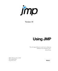
Figure 2.1 Example of a Control Chart

Contents 

Statistical Quality Control with Control Charts . . . . . . . . . . . . . . . . . . . . . . . . . . . . . . . . . . . . . . . . . . . 27 

The Control Chart Launch Dialog . . . . . . . . . . . . . . . . . . . . . . . . . . . . . . . . . . . . . . . . . . . . . . . . . . . . . 27 

Process Information. . . . . . . . . . . . . . . . . . . . . . . . . . . . . . . . . . . . . . . . . . . . . . . . . . . . . . . . . . . . . . .28 

Chart Type Information . . . . . . . . . . . . . . . . . . . . . . . . . . . . . . . . . . . . . . . . . . . . . . . . . . . . . . . . . . . 31 

Parameters . . . . . . . . . . . . . . . . . . . . . . . . . . . . . . . . . . . . . . . . . . . . . . . . . . . . . . . . . . . . . . . . . . . . . .32 

Using Specified Statistics . . . . . . . . . . . . . . . . . . . . . . . . . . . . . . . . . . . . . . . . . . . . . . . . . . . . . . . . . . .33 

Tailoring the Horizontal Axis . . . . . . . . . . . . . . . . . . . . . . . . . . . . . . . . . . . . . . . . . . . . . . . . . . . . . . . . . .34 

Display Options . . . . . . . . . . . . . . . . . . . . . . . . . . . . . . . . . . . . . . . . . . . . . . . . . . . . . . . . . . . . . . . . . . . .34 

Single Chart Options . . . . . . . . . . . . . . . . . . . . . . . . . . . . . . . . . . . . . . . . . . . . . . . . . . . . . . . . . . . . .34 

Window Options . . . . . . . . . . . . . . . . . . . . . . . . . . . . . . . . . . . . . . . . . . . . . . . . . . . . . . . . . . . . . . . .37 

Tests for Special Causes . . . . . . . . . . . . . . . . . . . . . . . . . . . . . . . . . . . . . . . . . . . . . . . . . . . . . . . . . . . . . . .39 

Nelson Rules . . . . . . . . . . . . . . . . . . . . . . . . . . . . . . . . . . . . . . . . . . . . . . . . . . . . . . . . . . . . . . . . . . . .39 

Westgard Rules . . . . . . . . . . . . . . . . . . . . . . . . . . . . . . . . . . . . . . . . . . . . . . . . . . . . . . . . . . . . . . . . . 42 

Running Alarm Scripts . . . . . . . . . . . . . . . . . . . . . . . . . . . . . . . . . . . . . . . . . . . . . . . . . . . . . . . . . . . . . . 44 

Saving and Retrieving Limits. . . . . . . . . . . . . . . . . . . . . . . . . . . . . . . . . . . . . . . . . . . . . . . . . . . . . . . . . . .45 

Real-Time Data Capture . . . . . . . . . . . . . . . . . . . . . . . . . . . . . . . . . . . . . . . . . . . . . . . . . . . . . . . . . . . . . 49 

The Open Datafeed Command. . . . . . . . . . . . . . . . . . . . . . . . . . . . . . . . . . . . . . . . . . . . . . . . . . . . . 49 

Commands for Data Feed . . . . . . . . . . . . . . . . . . . . . . . . . . . . . . . . . . . . . . . . . . . . . . . . . . . . . . . . . 49 

Operation . . . . . . . . . . . . . . . . . . . . . . . . . . . . . . . . . . . . . . . . . . . . . . . . . . . . . . . . . . . . . . . . . . . . . 50 

Setting Up a Script to Start a New Data Table. . . . . . . . . . . . . . . . . . . . . . . . . . . . . . . . . . . . . . . . . . 50 

Setting Up a Script in a Data Table . . . . . . . . . . . . . . . . . . . . . . . . . . . . . . . . . . . . . . . . . . . . . . . . . . . 51 

Excluded, Hidden, and Deleted Samples . . . . . . . . . . . . . . . . . . . . . . . . . . . . . . . . . . . . . . . . . . . . . . . . . . 51

Chapter 2 Statistical Control Charts 27 

Statistical Quality Control with Control Charts 

Statistical Quality Control with Control Charts 

Control charts are a graphical and analytic tool for deciding whether a process is in a state of statistical 

control and for monitoring an in-control process. 

Control charts have the following characteristics: 

• Each point represents a summary statistic computed from a subgroup sample of measurements of a 

quality characteristic. 

Subgroups should be chosen rationally, that is, they should be chosen to maximize the probability of 

seeing a true process signal between subgroups. 

• The vertical axis of a control chart is scaled in the same units as the summary statistic. 

• The horizontal axis of a control chart identifies the subgroup samples. 

• The center line on a Shewhart control chart indicates the average (expected) value of the summary 

statistic when the process is in statistical control. 

• The upper and lower control limits, labeled UCL and LCL, give the range of variation to be expected in 

the summary statistic when the process is in statistical control. 

• A point outside the control limits (or the V-mask of a CUSUM chart) signals the presence of a special 

cause of variation. 

• Analyze > Quality And Process > Control Chart subcommands create control charts that can be 

updated dynamically as samples are received and recorded or added to the data table. 

Figure 2.2 Description of a Control Chart 

Out of Control Point 

Measurement 

Axis 

UCL 

Center Line 

LCL 

Subgroup Sample Axis 

The Control Chart Launch Dialog 

When you select a Control Chart from the Analyze > Quality And Process > Control Chart, you see a 

Control Chart Launch dialog similar to the one in Figure 2.3. (The exact controls vary depending on the 

type of chart you choose.) Initially, the dialog shows three kinds of information: 

• Process information, for measurement variable selection

28 Statistical Control Charts Chapter 2 


• Chart type information 

• Limits specification 

Specific information shown for each section varies according to the type of chart you request. 

Figure 2.3 XBar Control Chart Launch Dialog 

process 

information 

chart type 

information 

limits 

specification 

Add capability analysis 

to the report. 

Enter or remove 

known statistics. 

Through interaction with the Launch dialog, you specify exactly how you want your charts created. The 

following sections describe the panel elements. 

Process Information 

Process 

The Launch dialog displays a list of columns in the current data table. Here, you specify the variables to be 

analyzed and the subgroup sample size. 

The Process role selects variables for charting. 

• For variables charts, specify measurements as the process. 

• For attribute charts, specify the defect count or defective proportion as the process. The data will be 

interpreted as counts, unless it contains non-integer values between 0 and 1. 

Note: The rows of the table must be sorted in the order you want them to appear in the control chart. Even 

if there is a Sample Label variable specified, you still must sort the data accordingly.



Sample Label 

The Sample Label role enables you to specify a variable whose values label the horizontal axis and can also 

identify unequal subgroup sizes. If no sample label variable is specified, the samples are identified by their 

subgroup sample number. 

• If the sample subgroups are the same size, check the Sample Size Constant radio button and enter the 

size into the text box. If you entered a Sample Label variable, its values are used to label the horizontal 

axis. The sample size is used in the calculation of the limits regardless of whether the samples have 

missing values. 

• If the sample subgroups have an unequal number of rows or have missing values and you have a column 

identifying each sample, check the Sample Grouped by Sample Label radio button and enter the 

sample identifying column as the sample label. 

For attribute charts (P-, NP-, C-, and U-charts), this variable is the subgroup sample size. In Variables 

charts, it identifies the sample. When the chart type is IR, a Range Span text box appears. The range span 

specifies the number of consecutive measurements from which the moving ranges are computed. 

Note: The rows of the table must be sorted in the order you want them to appear in the control chart. Even 

if there is a Sample Label variable specified, you still must sort the data accordingly. 

The illustration in Figure 2.4 shows an X -chart for a process with unequal subgroup sample sizes, using the 

Coating.jmp sample data from the Quality Control sample data folder.



Figure 2.4 Variables Charts with Unequal Subgroup Sample Sizes 

Phase 

The Phase role enables you to specify a column identifying different phases, or sections. A phase is a group 

of consecutive observations in the data table. For example, phases might correspond to time periods during 

which a new process is brought into production and then put through successive changes. Phases generate, 

for each level of the specified Phase variable, a new sigma, set of limits, zones, and resulting tests. See 

“Phases” on page 91 in the “Shewhart Control Charts” chapter for complete details of phases. For the 

Diameter.jmp data, found in the Quality Control sample data folder, launch an XBar Control Chart. Then 

specify Diameter as Process, Day as Sample Label, Phase as Phase, and check the box beside S for an S 

control chart to obtain the two phases shown in Figure 2.5.



Figure 2.5 XBar and S Charts with Two Phases 

Chart Type Information 

Shewhart control charts are broadly classified as variables charts and attribute charts. Moving average charts 

and cusum charts can be thought of as special kinds of variables charts.



Figure 2.6 Dialog Options for Variables Control Charts 

XBar, R, and S 

IR 

EWMA 

CUSUM 

UWMA 

Presummarize 

Parameters 

KSigma 

• XBar charts menu selection gives XBar, R, and S checkboxes. 

• The IR menu selection has checkbox options for the Individual Measurement, Moving Range, and 

Median Moving Range charts. 

• The uniformly weighted moving average (UWMA) and exponentially weighted moving average (EWMA) 

selections are special charts for means. 

• The CUSUM chart is a special chart for means or individual measurements. 

• Presummarize allows you to specify information on pre-summarized statistics. 

• P, NP, C, and U charts, Run Chart, and Levey-Jennings charts have no additional specifications. 

The types of control charts are discussed in “Shewhart Control Charts” on page 69. 

You specify computations for control limits by entering a value for k (K Sigma), or by entering a probability 

for α(Alpha), or by retrieving a limits value from the process columns' properties or a previously created 

Limits Table. Limits Tables are discussed in the section “Saving and Retrieving Limits” on page 45, later in 

this chapter. There must be a specification of either K Sigma or Alpha. The dialog default for K Sigma is 3. 

The KSigma parameter option allows specification of control limits in terms of a multiple of the sample 

standard error. KSigma specifies control limits at k sample standard errors above and below the expected 

value, which shows as the center line. To specify k, the number of sigmas, click the radio button for KSigma 

and enter a positive k value into the text box. The usual choice for k is 3, which is three standard deviations.



The examples shown in Figure 2.7 compare the X -chart for the Coating.jmp data with control lines drawn 

with KSigma =3 and KSigma =4. 

Figure 2.7 K Sigma =3 (left) and K Sigma=4 (right) Control Limits 

Alpha 

The Alpha parameter option specifies control limits (also called probability limits) in terms of the probability 

α that a single subgroup statistic exceeds its control limits, assuming that the process is in control. To specify 

alpha, click the Alpha radio button and enter the probability you want. Reasonable choices for α are 0.01 or 

0.001. The Alpha value equivalent to a KSigma of 3 is 0.0027. 

Using Specified Statistics 

After specifying a process variable, if you click the Specify Stats (when available) button on the Control 

Chart Launch dialog, a tab with editable fields is appended to the bottom of the launch dialog. This lets you 

enter historical statistics (statistics obtained from historical data) for the process variable. The Control Chart 

platform uses those entries to construct control charts. The example here shows 1 as the standard deviation 

of the process variable and 20 as the mean measurement. 

Figure 2.8 Example of Specify Stats 

Note: When the mean is user-specified, it is labeled in the plot as μ0.


Tailoring the Horizontal Axis 

If you check the Capability option on the Control Chart launch dialog (see Figure 2.3), a dialog appears as 

the platform is launched asking for specification limits. The standard deviation for the control chart selected 

is sent to the dialog and appears as a Specified Sigma value, which is the default option. After entering the 

specification limits and clicking OK, capability output appears in the same window next to the control 

chart. For information on how the capability indices are computed, see the Basic Analysis and Graphing 

book. 

Tailoring the Horizontal Axis 

When you double-click the x axis, the X Axis Specification dialog appears for you to specify the format, axis 

values, number of ticks, gridline and reference lines to display on the x axis. 

For example, the Pickles.JMP data lists measurements taken each day for three days. In this example, by 

default, the x axis is labeled at every other tick. Sometimes this gives redundant labels, as shown to the left in 

Figure 2.9. If you specify a label at an increment of eight, with seven ticks between them, the x axis is labeled 

once for each day, as shown in the chart on the right. 

Figure 2.9 Example of Labeled x Axis Tick Marks 

Display Options 

Control Charts have popup menus that affect various parts of the platform: 

• The menu on the top-most title bar affects the whole platform window. Its items vary with the type of 

chart you select. 

• There is a menu of items on the chart type title bar with options that affect each chart individually. 

Single Chart Options 

The popup menu of chart options appears when you click the icon next to the chart name, or context-click 

the chart space (right-mouse click on Windows or Control-click on the Macintosh). The CUSUM chart has



different options that are discussed in “Cumulative Sum Control Charts” on page 95. 

Box Plots superimposes box plots on the subgroup means plotted in a Mean chart. The box plot shows 

the subgroup maximum, minimum, 75th percentile, 25th percentile, and median. Markers for 

subgroup means show unless you deselect the Show Points option. The control limits displayed apply 

only to the subgroup mean. The Box Plots option is available only for X -charts. It is most appropriate 

for larger subgroup sample sizes (more than 10 samples in a subgroup). 

Needle 

connects plotted points to the center line with a vertical line segment. 

Connect Points 

toggles between connecting and not connecting the points. 

Show Points toggles between showing and not showing the points representing summary statistics. 

Initially, the points show. You can use this option to suppress the markers denoting subgroup means 

when the Box Plots option is in effect. 

Connect Color displays the JMP color palette for you to choose the color of the line segments used to 

connect points. 

Center Line Color displays the JMP color palette for you to choose the color of the line segments used to 

draw the center line. 

Limits Color displays the JMP color palette for you to choose the color of the line segments used in the 

upper and lower limits lines. 

Line Width 

allows you to pick the width of the control lines. Options are Thin, Medium, or Thick. 

Point Marker 

allows you to pick the marker used on the chart. 

Show Center Line initially displays the center line in green. Deselecting Show Center Line removes the 

center line and its legend from the chart. 

Show Control Limits 

legends. 

toggles between showing and not showing the chart control limits and their 

Tests shows a submenu that enables you to choose which tests to mark on the chart when the test is 

positive. Tests apply only for charts whose limits are 3σ limits. Tests 1 to 4 apply to Mean, Individual 

and attribute charts. Tests 5 to 8 apply to Mean charts, Presummarize, and Individual Measurement 

charts only. If tests do not apply to a chart, the Tests option is dimmed. Tests apply, but will not appear 

for charts whose control limits vary due to unequal subgroup sample sizes, until the sample sizes become 

equal. These special tests are also referred to as the Nelson Rules. For more information on special causes 

tests, see “Tests for Special Causes” on page 39 later in this chapter. 

Westgard Rules are detailed below. See the text and chart in “Westgard Rules” on page 42. 

Test Beyond Limits flags as a “*” any point that is beyond the limits. This test works on all charts with 

limits, regardless of the sample size being constant, and regardless of the size of k or the width of the 

limits. For example, if you had unequal sample sizes, and wanted to flag any points beyond the limits of 

an r-chart, you could use this command.



Show Zones toggles between showing and not showing the zone lines. The zones are labeled A, B, and C 

as shown here in the Mean plot for weight in the Coating.jmp sample data. Control Chart tests use the 

zone lines as boundaries. The seven zone lines are set one sigma apart, centered on the center line. 

Figure 2.10 Show Zones 

Shade Zones toggles between showing and not showing the default green, yellow, and red colors for the 

three zone areas and the area outside the zones. Green represents the area one sigma from the center line, 

yellow represents the area two and three sigmas from the center line, and red represents the area beyond 

three sigma. Shades may be shown with or without the zone lines. 

Figure 2.11 Shade Zones 

OC Curve gives Operating Characteristic (OC) curves for specific control charts. OC curves are defined 

in JMP only for X -, P-, NP-, C-, and U-charts. The curve shows how the probability of accepting a lot 

changes with the quality of the sample. When you choose the OC Curve option from the control chart 

option list, JMP opens a new window containing the curve, using all the calculated values directly from 

the active control chart. Alternatively, you can run an OC curve directly from the Control category of 

the JMP Starter. Select the chart on which you want the curve based, then a dialog prompts you for 

Target, Lower Control Limit, Upper Control Limit, k, Sigma, and Sample Size. You can also perform 

both single and double acceptance sampling in the same manner. To engage this feature, choose



Window Options 

View > JMP Starter > Control (under Click Category) > OC Curves. A pop-up dialog box allows you 

to specify whether or not single or double acceptance sampling is desired. A second pop-up dialog is 

invoked, where you can specify acceptance failures, number inspected, and lot size (for single acceptance 

sampling). Clicking OK generates the desired OC curve. 

The popup menu on the window title bar lists options that affect the report window. The example menu 

shown here appears if you request XBar and R at the same time. You can check each chart to show or hide it. 

Figure 2.12 Report Options 

The specific options that are available depend on the type of control chart you request. Unavailable options 

show as grayed menu items. 

The following options show for all control charts except Run Charts: 

Show Limits Legend 

shows or hides the Avg, UCL, and LCL values to the right of the chart. 

Connect Through Missing connects points when some samples have missing values. In Figure 2.13, the 

left chart has no missing points. The middle chart has samples 2, 11, 19, and 27 missing with the points 

not connected. The right chart appears if you select the Connect Through Missing option, which is the 

default. 

Figure 2.13 Example of Connected Through Missing Option 

no missing points Missing points are not connected. Missing points are connected.



Capability performs a Capability Analysis for your data. A popup dialog is first shown, where you can 

enter the Lower Spec Limit, Target, and Upper Spec Limit values for the process variable. 

Figure 2.14 Capability Analysis Dialog 

An example of a capability analysis report is shown in Figure 2.15 for Coating.jmp when the Lower Spec 

Limit is set as 16.5, the Target is set to 21.5, and the Upper Spec Limit is set to 23. 

Figure 2.15 Capability Analysis Report for Coating.jmp 

For additional information on Capability Analysis, see the Basic Analysis and Graphing book. 

Save Sigma saves the computed value of sigma as a column property in the process variable column in 

the JMP data table. 

Save Limits > in Column saves the computed values of sigma, center line, and the upper and lower limits 

as column properties in the process variable column in the JMP data table. These limits are later 

automatically retrieved by the Control Chart dialog and used in a later analysis.


Tests for Special Causes 

Figure 2.16 Properties in the Column Info Window 

Save Limits > in New Table saves all parameters for the particular chart type, including sigma and K 

Sigma, sample size, the center line, and the upper and lower control limits in a new JMP data table. 

These limits can be retrieved by the Control Chart dialog and used in a later analysis. See the section 

“Saving and Retrieving Limits” on page 45 for more information. 

Save Summaries creates a new data table that contains the sample label, sample sizes, the statistic being 

plotted, the centerline, and the control limits. The specific statistics included in the table depend on the 

type of chart. 

Alarm Script displays a dialog for choosing or entering a script or script name and executes by either 

writing to the log or speaking whenever the tests for special causes is in effect and a point is out of range. 

See section “Tests for Special Causes” on page 39 for more information. See “Running Alarm Scripts” on 

page 44 for more information on writing custom Alarm Scripts. 

Script 

contains options that are available to all platforms. See Using JMP. 


The Tests option in the chart type popup menu displays a submenu for test selection. You can select one or 

more tests for special causes with the options popup menu. Nelson (1984) developed the numbering 

notation used to identify special tests on control charts. 

If a selected test is positive for a particular sample, that point is labeled with the test number. When you 

select several tests for display and more than one test signals at a particular point, the label of the 

numerically lowest test specified appears beside the point. 

Nelson Rules 

The Nelson rules are implemented in the Tests submenu. Table 2.1 on page 40 lists and interprets the 

eight tests, and Figure 2.18 illustrates the tests. The following rules apply to each test: 

• The area between the upper and lower limits is divided into six zones, each with a width of one standard 

deviation. 

• The zones are labeled A, B, C, C, B, A with zones C nearest the center line. 

• A point lies in Zone B or beyond if it lies beyond the line separating zones C and B. That is, if it is more 

than one standard deviation from the center line.



• Any point lying on a line separating two zones lines is considered belonging to the outermost zone. 

Note: All Tests and zones require equal sample sizes in the subgroups of nonmissing data. 

Tests 1 through 8 apply to Mean ( X ) and individual measurement charts. Tests 1 through 4 can also apply 

to P-, NP-, C-, and U-charts. 

Tests 1, 2, 5, and 6 apply to the upper and lower halves of the chart separately. Tests 3, 4, 7, and 8 apply to 

the whole chart. 

See Nelson (1984, 1985) for further recommendations on how to use these tests. 

Figure 2.17 Zones for Nelson Rules 

3σ limits 

zones 

center line 

Table 2.1 Description and Interpretation of Special Causes Tests a 

Test 1 One point beyond Zone A detects a shift in the mean, an increase in the standard 

deviation, or a single aberration in the process. For 

interpreting Test 1, the R-chart can be used to rule out 

increases in variation. 

Test 2 

Test 3 

Test 4 

Test 5 

Nine points in a row in a single 

(upper or lower) side of Zone C 

or beyond 

Six points in a row steadily 

increasing or decreasing 

Fourteen points in a row 

alternating up and down 

Two out of three points in a row 

in Zone A or beyond and the 

point itself is in Zone A or 

beyond. 

detects a shift in the process mean. 

detects a trend or drift in the process mean. Small trends 

will be signaled by this test before Test 1. 

detects systematic effects such as two alternately used 

machines, vendors, or operators. 

detects a shift in the process average or increase in the 

standard deviation. Any two out of three points provide a 

positive test.



Table 2.1 Description and Interpretation of Special Causes Tests a (Continued) 

Test 6 

Test 7 

Test 8 

Four out of five points in a row 

in Zone B or beyond and the 

point itself is in Zone B or 

beyond. 

Fifteen points in a row in Zone 

C, above and below the center 

line 

Eight points in a row on both 

sides of the center line with none 

in Zones C 

detects a shift in the process mean. Any four out of five 

points provide a positive test. 

detects stratification of subgroups when the observations 

in a single subgroup come from various sources with 

different means. 

detects stratification of subgroups when the observations 

in one subgroup come from a single source, but 

subgroups come from different sources with different 

means. 

a. Nelson (1984, 1985)



Figure 2.18 Illustration of Special Causes Tests 1 

Test 1: One point beyond Zone A 

A 

B 

C 

C 

B 

A 

1 

UCL 

Avg 

LCL 

Test 3: Six points in a row steadily increasing 

or decreasing 

A 

B 

C 

C 

B 

A 

3 

UCL 

Avg 

LCL 

Test 2: Nine points in a row in a single (upper 

or lower) side of Zone C or beyond 

A 

UCL 

B 

C 

C 

B 

A 

2 

Avg 

LCL 

Test 4: Fourteen points in a row alternating 

up and down 

A 

UCL 

B 

C 

C 

B 

A 

4 Avg 

LCL 

Test 5: Two out of three points in a row in Test 6: Four out of five points in a row in 

Zone A or beyond 

Zone B or beyond 

A 5 

UCL 

5 A 

6 

UCL 

B 

B 

C 

Avg C 

C 

C 

Avg 

B 

A 

5 

LCL 

B 

A 

LCL 

Test 7: Fifteen points in a row in Zone C 

(above and below the center line) 

A 

UCL 

B 

C 

7 Avg 

C 

B 

A 

LCL 

Test 8: Eight points in a row on both sides of 

the center line with none in Zone C 

A 

UCL 

B 

C 

Avg 

C 

B 

8 

A 

LCL 

Westgard Rules 

Westgard rules are implemented under the Westgard Rules submenu of the Control Chart platform. The 

different tests are abbreviated with the decision rule for the particular test. For example, 1 2s refers to a test 

where one point is two standard deviations away from the mean. 

1. Nelson (1984, 1985)



Table 2.2 Westgard Rules 

Rule 1 2S is commonly used with Levey-Jennings charts, 

where control limits are set 2 standard deviations away 

from the mean. The rule is triggered when any one point 

goes beyond these limits. 

Rule 1 3S refers to a rule common to Levey-Jennings 

charts where the control limits are set 3 standard 

deviations away from the mean. The rule is triggered 

when any one point goes beyond these limits. 

Rule 2 2S is triggered when two consecutive control 

measurements are farther than two standard deviations 

from the mean. 

Rule R 4S is triggered when one measurement is greater 

than two standard deviations from the mean and the 

previous measurement is greater than two standard 

deviations from the mean in the opposite direction such 

that the difference is greater than 4 standard deviations. 

Rule 4 1S is triggered when four consecutive 

measurements are more than one standard deviation from 

the mean. 

Rule 10 X is triggered when ten consecutive points are on 

one side of the mean. 

+3s 

+2s 

+1s 

-1s 

-2s 

-3s 

+3s 

+2s 

+1s 

-1s 

-2s 

-3s 

+3s 

+2s 

+1s 

-1s 

-2s 

-3s 

+3s 

+2s 

+1s 

-1s 

-2s 

-3s 

+3s 

+2s 

+1s 

-1s 

-2s 

-3s 

+3s 

+2s 

+1s 

-1s 

-2s 

-3s 

UCL 

Avg 

LCL 

UCL 

Avg 

LCL 

UCL 

Avg 

LCL 

UCL 

Avg 

LCL 

UCL 

Avg 

LCL 

UCL 

Avg 

LCL


Running Alarm Scripts 

Running Alarm Scripts 

If you want to run a script that alerts you when the data fail one or more tests, you can run an Alarm Script. 

As an Alarm Script is invoked, the following variables are available, both in the issued script and in 

subsequent JSL scripts: 

qc_col is the name of the column 

qc_test is the test that failed 

qc_sample is the sample number 

qc_firstRow is the first row in the sample 

qc_lastRow is the last row in the sample 

Example 1: Automatically writing to a log 

One way to generate automatic alarms is to make a script and store it with the data table as a Data Table 

property named QC Alarm Script. To automatically write a message to the log whenever a test fails, 

• Run the script below to save the script as a property to the data table, 

• Run a control chart, 

• Turn on the tests you're interested in. If there are any samples that failed, you'll see a message in the log. 

CurrentData Table()


Saving and Retrieving Limits 

You can have either of these scripts use any of the JSL alert commands such as Speak, Write or Mail. 

Note: Under Windows, in order to have sound alerts you must install the Microsoft Text-to-Speech engine, 

which is included as an option with the JMP product installation. 


JMP can use previously established control limits for control charts: 

• upper and lower control limits, and a center line value 

• parameters for computing limits such as a mean and standard deviation. 

The control limits or limit parameter values must be either in a JMP data table, referred to as the Limits 

Table or stored as a column property in the process column. When you specify the Control Chart 

command, you can retrieve the Limits Table with the Get Limits button on the Control Chart launch 

dialog. 

The easiest way to create a Limits Table is to save results computed by the Control Chart platform. The 

Save Limits command in the popup menu for each control chart automatically saves limits from the sample 

values. The type of data saved in the table varies according to the type of control chart in the analysis 

window. You can also use values from any source and create your own Limits Table. All Limits Tables must 

have 

• a column of special key words that identify each row 

• a column for each of the variables whose values are the known standard parameters or limits. This 

column name must be the same as the corresponding process variable name in the data table to be 

analyzed by the Control Chart platform. 

You can save limits in a new data table or as properties of the response column. When you save control 

limits using the in New Table command, the limit key words written to the table depend on the current 

chart types displayed. 

Figure 2.19 shows examples of control limits saved to a data table. The rows with values _Mean, _LCL, and 

_UCL are for the Individual Measurement chart. The values with the R suffix (_AvgR, _LCLR, and _UCLR) 

are for the Moving Range chart. If you create these charts again using this Limits Table, the Control Chart 

platform identifies the appropriate limits from key words in the _LimitsKey column.



Figure 2.19 Example of Saving Limits in a Data Table 

A list of limit key words and their associated control chart is shown in Table 2.3 on page 47. 

Note that values for _KSigma, _Alpha, and _Range Span can be specified in the Control Chart Launch 

dialog. JMP always looks at the values from the dialog first. Values specified in the dialog take precedence 

over those in an active Limits Table. 

The Control Chart command ignores rows with unknown key words and rows marked with the excluded 

row state. Except for _Range Span, _KSigma, _Alpha, and _Sample Size, any needed values not specified 

are estimated from the data. 

As an aid when referencing Table 2.3 on page 47, the following list summarizes the kinds of charts 

available in the Control Chart platform: 

• Run charts 

• Variables charts are the following types: 

– X -chart (Mean) 

– R-chart (range) 

– S-chart (standard deviation) 

– IM chart (individual measurement) 

– MR chart (moving range) 

– UWMA chart (uniformly weighted moving average)



– EWMA chart (exponentially weighted moving average) 

– CUSUM chart (cumulative sum) 

– Levey-Jennings chart (Mean) 

• Attribute charts are the following types: 

– P-chart (proportion of nonconforming or defective items in a subgroup sample) 

– NP-chart (number of nonconforming or defective items in a subgroup sample) 

– C-chart (number of nonconformities or defects in a subgroup sample) 

– U-chart (number of nonconforming or defects per unit). 

Table 2.3 Limits Table Keys with Appropriate Charts and Meanings 

Key Words For Chars Meaning 

_Sample Size 

X , R-, S-, P-, NP-, C-, U-, 

UWMA, EWMA, 

CUSUM 

fixed sample size for control limits; set to 

missing if the sample size is not fixed. If 

specified in the Control Chart launch 

dialog, fixed sample size is displayed. 

_Range Span IM, MR specifies the number ( 2 ≤ n ≤ 25 ) of 

consecutive values for computation of 

moving range 

_Span UWMA specifies the number ( 2 ≤ n ≤ 25 ) of 

consecutive subsample means for 

computation of moving average 

_Weight EWMA constant weight for computation of 

EWMA 

_KSigma All multiples of the standard deviation of the 

statistics to calculate the control limits; set 

to missing if the limits are in terms of the 

alpha level 

_Alpha All Type I error probability used to calculate 

the control limits; used if multiple of the 

standard deviation is not specified in the 

launch dialog or in the Limits Table 

_Std Dev 

_Mean 

X -, R-, S-, IM, MR, 

UWMA, EWMA, 

CUSUM 

X -, IM, UWMA, EWMA, 

CUSUM 

known process standard deviation 

known process mean



Table 2.3 Limits Table Keys with Appropriate Charts and Meanings (Continued) 

Key Words For Chars Meaning 

_U C-, U- known average number of nonconformities 

per unit 

_P NP-, P- known value of average proportion 

nonconforming 

_LCL, _UCL X -, IM, P-, NP-, C-, U- lower and upper control limit for Mean 

Chart, Individual Measurement chart, or 

any attribute chart 

_AvgR R-, MR average range or average moving range 

_LCLR, _UCLR R-, MR lower control limit for R- or MR chart 

upper control limit for R- or MR chart 

_AvgS, _LCLS, _UCLS S-Chart average standard deviation, upper and 

lower control limits for S-chart 

_Head Start CUSUM head start for one-sided scheme 

_Two Sided, _Data Units CUSUM type of chart 

_H, _K CUSUM alternative to alpha and beta; K is optional 

_Delta 

_Beta 

_AvgR_PreMeans 

_AvgR_PreStdDev 

_LCLR_PreMeans 

_LCLR_PreStdDev 

_UCLR_PreMeans 

_UCLR_PreStdDev 

_Avg_PreMeans 

_Avg_PreStdDev 

_LCL_PreMeans 

_LCL_PreStdDev 

_UCL_PreMeans 

_UCL_PreStdDev 

CUSUM 

IM, MR 

Absolute value of the smallest shift to be 

detected as a multiple of the process 

standard deviation or standard error 

probability and are available only when 

_Alpha is specified. 

Mean, upper and lower control limits based 

on pre-summarized group means or 

standard deviations.


Real-Time Data Capture 


In JMP, real-time data streams are handled with a DataFeed object set up through JMP Scripting Language 

(JSL) scripts. The DataFeed object sets up a concurrent thread with a queue for input lines that can arrive 

in real time, but are processed during background events. You set up scripts to process the lines and push 

data on to data tables, or do whatever else is called for. Full details for writing scripts are in the JMP Scripting 

Language Guide. 

The Open Datafeed Command 

To create a DataFeed object, use the Open DataFeed function specifying details about the connection, in 

the form 

feedname = Open DataFeed( options... ); 

For example, submit this to get records from com1 and just list them in the log. 

feed = OpenDataFeed( 

Connect( Port("com1:"),Baud(9600),DataBits(7)), 

SetScript(print(feed



Operation 

where the port specifications inside the Connect command are as follows. Each option takes only one 

argument, but they are shown below with the possible arguments separated by “|” with the default value 

shown first. The last three options take boolean values that specify which control characters are sent back 

and forth to the device indicating when it is ready to get data. Usually, at most, one of these three is used: 

Port( "com1:" | "com2:" | "lpt1:" |...), 

Baud( 9600 | 4800 | ...), 

Data Bits( 8 | 7 ), 

Parity( None | Odd | Even ), 

Stop Bits( 1 | 0 | 2 ), 

DTR_DSR( 0 | 1 ), // DataTerminalReady 

RTS_CTS( 0 | 1 ), // RequestToSend/ClearToSend 

XON_XOFF( 1 | 0 ) 

The Port specification is needed if you want to connect; otherwise, the object still works but is not 

connected to a data feed. 

To disconnect from the live data source: 

feedName


Excluded, Hidden, and Deleted Samples 

dc = dt


Excluded, Hidden, and Deleted Samples 

Table 2.4 Excluded, Hidden, and Deleted Samples (Continued) 

All rows of the sample are both excluded 

and hidden before creating the chart. 

All rows of the sample are both excluded 

and hidden after creating the chart. 

Data set is subsetted with Sample 

deleted before creating chart. 

Data set is subsetted with Sample 

deleted after creating chart. 

Sample is not included in the calculation of the limits, and it 

does not appear on the graph. 

Sample is included in the calculation of the limits, but does 

not appear on the graph. The sample marker will disappear 

from the graph, the sample label will still appear on the axis, 

but limits remain the same. 

Sample is not included in the calculation of the limits, the 

axis will not include a value for the sample, and the sample 

marker does not appear on the graph. 

Sample is not included in the calculation of the limits, and 

does not appear on the graph. The sample marker will 

disappear from the graph, the sample label will still be 

removed from the axis, the graph will shift, and the limits 

will change. 

Some additional notes: 

• Hide operates only on the rowstate of the first observation in the sample. For example, if the second 

observation in the sample is hidden, while the first observation is not hidden, the sample will still appear 

on the chart. 

• An exception to the exclude/hide rule: Tests for Special Causes can flag if a sample is excluded, but will 

not flag if a sample is hidden. 

• Because of the specific rules in place (see Table 2.4 on page 51), the control charts do not support the 

Automatic Recalc script.

Chapter 3 

Introduction to Control Charts 

Control Chart Platforms 

Control charts are a way to quickly visualize process measurements over time, and filter out routine 

variation. This chapter describes the JMP approach to creating control charts, including a new interactive 

control chart platform called Control Chart Builder. 

Figure 3.1 Example of a Control Chart

Contents 

What is a Control Chart? . . . . . . . . . . . . . . . . . . . . . . . . . . . . . . . . . . . . . . . . . . . . . . . . . . . . . . . . . . . . . 55 

Parts of a Control Chart . . . . . . . . . . . . . . . . . . . . . . . . . . . . . . . . . . . . . . . . . . . . . . . . . . . . . . . . . . . . . . 55 

Control Charts in JMP . . . . . . . . . . . . . . . . . . . . . . . . . . . . . . . . . . . . . . . . . . . . . . . . . . . . . . . . . . . . . . .56 

Types and Availability on Chart Charts . . . . . . . . . . . . . . . . . . . . . . . . . . . . . . . . . . . . . . . . . . . . . . . . . . .57

Chapter 3 Introduction to Control Charts 55 

What is a Control Chart? 

What is a Control Chart? 

A control chart is a graphical way to filter out routine variation in a process. Filtering out routine variation 

helps manufacturers and other businesses determine whether a process is stable and predictable. If the 

variation is more than routine, the process can be adjusted to create higher quality output at a lower cost. 

All processes exhibit variation as the process is measured over time. There are two types of variation in 

process measurements: 

• Routine or common-cause variation. Even measurements from a stable process exhibit these random ups 

and downs. When process measurements exhibit only common-cause variation, the measurements stay 

within acceptable limits. 

• Abnormal or special-cause variation. Examples of special-cause variation include a change in the process 

mean, points above or below the control limits, or measurements that trend up or down. These changes 

can be caused by factors such as a broken tool or machine, equipment degradation, and changes to raw 

materials. A change or defect in the process is often identifiable by abnormal variation in the process 

measurements. 

Control charts quantify the routine variation in a process, so that special causes can be identified. One way 

control charts filter out routine variation is by applying control limits. Control limits define the range of 

process measurements for a process that is exhibiting only routine variation. Measurements between the 

control limits indicate a stable and predictable process. Measurements outside the limits indicate a special 

cause, and action should be taken to restore the process to a state of control. 

Control chart performance is dependent on the sampling scheme used. The sampling plan should be 

rational, that is, the subgroups are representative of the process. Rational subgrouping means that you will 

sample from the process by picking subgroups in such a way that special causes are more likely to occur 

between subgroups rather than within subgroups. 

Parts of a Control Chart 

A control chart is a plot of process measurements over time, with control limits added to help separate 

routine and abnormal variation. Figure 3.2 describes the parts of a simple control chart.

56 Introduction to Control Charts Chapter 3 

Control Charts in JMP 

Figure 3.2 Parts of a Basic Control Chart 

out-of-control point 

upper control limit 

centerline 

lower control limit 

Note the following about control charts: 

• Each point plotted on the chart represents an individual process measurement or summary statistic. In 

this example, the points represent the average for a sample of measurements. 

• The X axis of the control chart is time ordered. Observing the process over time is important in assessing 

if the process is changing. 

• The two red lines are the upper and lower control limits. If the process is exhibiting only routine 

variation, then all the points should fall randomly in that range. In this example, one measurement is 

above the upper control limit. This is evidence that the measurement could have been influenced by a 

special cause, or is possibly a defect. 

• The green line is the center line, or the average of the data. Measurements should appear equally on both 

sides of the center line. If not so, this is possible evidence that the process average is changing. 

When a control chart signals abnormal variation, action should be taken to return the process to a state of 

statistical control if the process degraded. If the abnormal variation indicates an improvement in the process, 

the causes of the variation should be studied and implemented. 

Control Charts in JMP 

JMP 10 introduces a shift in the approach to control charts. We are moving toward an all-in-one, interactive 

workspace called Control Chart Builder. Control Chart Builder can be used to create several types of control 

charts, and is intended to be an interactive tool for problem solving and process analysis. 

To use Control Chart Builder, you do not need to know the name of a particular chart beforehand. When 

you drag a data column to the workspace, Control Chart Builder creates an appropriate chart based on the 

data type and sample size. Once the basic chart is created, use the right-click menu to: 

• change the statistic on the chart 

• format the chart 

• add additional charts

Chapter 3 Introduction to Control Charts 57 

Types and Availability on Chart Charts 

Note: The most common control charts are available in the classic platforms and the Control Chart 

Builder. Use the Control Chart Builder as your first choice to easily and quickly generate the charts. 


Several control chart types are available in the classic platforms and the new interactive Control Chart 

Builder. Table 3.1 shows all the types of control charts that are supported in JMP 10 and indicates whether 

each chart is available in the Control Chart Builder. 

Table 3.1 Control Chart Types 

Type Plotting Statistic In Control 

Chart Builder? 

Classic 

Platform 

Individual Individual measurements of the process. Yes IR 

Moving Range Moving range of individual points. Yes IR 

X-Bar Subgroup averages. Yes XBar 

Range Subgroup ranges. Yes XBar 

Standard 

Deviation 

Subgroup standard deviations. Yes XBar 

3-in-1 Chart 

Subgroup averages, within-subgroup 

variation, between-subgroup variation. 

Yes 

not available 

Presummarize 

Group means or standard deviations. 

This is used when you have repeated 

measurements on each process unit, and 

want to summarize into a single 

measurement for each unit before 

charting. 

Yes 

Presummarize 

Levey Jennings 

Individual measurements. The control 

limits are based on an estimate of 

long-term sigma. 

Yes 

Levey Jennings 

Run Chart 

Charts either the subgroup means or 

individual measurements only. 

No 

Run Chart 

P 

Proportion of defective units in a 

subgroup. 

No 

P 

NP 

Number of defective units in a 

subgroup. 

No 

NP

58 Introduction to Control Charts Chapter 3 


Table 3.1 Control Chart Types (Continued) 

Type Plotting Statistic In Control 

Chart Builder? 

Classic 

Platform 

C Number of defects in a subgroup. No C 

U 

Number of defects per unit in a 

subgroup. 

No 

U 

UWMA 

Moving average. The plotted point is 

the average of the last w subgroups. 

No 

UWMA 

EWMA 

Moving average. The plotted point is 

the weighted average of all previous 

subgroups. The weights decrease for 

older subgroups. 

No 

EWMA 

CUSUM Cumulative differences from a target. No CUSUM 

Multivariate 

T 2 statistics. This is used for 

simultaneous monitoring of multiple 

process variables on one chart. 

No 

Multivariate 

Control Chart

Chapter 4 

Interactive Control Charts 

The Control Chart Builder Platform 

Control Chart Builder provides a workspace where you can interactively investigate the stability of your 

process data using control charts. You can also compute control limits for different phases of a process. 

Several types of control charts are available, including: X-Bar, Individuals, Range, and Standard Deviation 

charts. 

Figure 4.1 Example of Control Chart Builder

Contents 

Overview of Control Chart Builder. . . . . . . . . . . . . . . . . . . . . . . . . . . . . . . . . . . . . . . . . . . . . . . . . . . . . .61 

Example Using Control Chart Builder . . . . . . . . . . . . . . . . . . . . . . . . . . . . . . . . . . . . . . . . . . . . . . . . . . .61 

Launch Control Chart Builder . . . . . . . . . . . . . . . . . . . . . . . . . . . . . . . . . . . . . . . . . . . . . . . . . . . . . . . . .63 

Control Chart Builder Options . . . . . . . . . . . . . . . . . . . . . . . . . . . . . . . . . . . . . . . . . . . . . . . . . . . . . . . . 64 

Additional Example of Control Chart Builder . . . . . . . . . . . . . . . . . . . . . . . . . . . . . . . . . . . . . . . . . . . . . 67 

Overview of Control Chart Builder. . . . . . . . . . . . . . . . . . . . . . . . . . . . . . . . . . . . . . . . . . . . . . . . . . . . . .61

Chapter 4 Interactive Control Charts 61 

Overview of Control Chart Builder 

Overview of Control Chart Builder 

Interact with Control Chart Builder to create control charts of your process data. Start with a blank 

workspace and drag and drop variables where you want them. The instant feedback encourages further 

exploration of the data. You can change your mind and quickly create another type of chart, or you can 

change the current settings by right-clicking on the existing chart. 

Use phase variables to produce different control limits for each phase. Use multiple variables to define 

subgroups. A report shows the average and control limits of each chart and phase. 

Some new features of the Control Chart Builder platform include the following: 

• ability to add, remove, and switch variables without relaunching the platform 

• ability to create subgroups that are defined by multiple X variables 

• three-in-one charts: subgroup means, within-subgroup variation, and between-subgroup variation 

• ability to create a chart without sorting data 

• JMP automatically chooses the appropriate chart type based on the data 

Note: The Control Chart Builder does not extend the size of one zone over another. If the limits are not 

centered around the mean, (UCL-Avg)/3 is used as the width of each zone. Zones are not drawn below the 

lower limit (LCL) or above the upper limit (UCL). 

Example Using Control Chart Builder 

You have data that includes measurements for the thickness of sockets. There has been an increase in the 

number of defects during production and you want to investigate why this is occurring. Use Control Chart 

Builder to investigate the variability in the data and the control of the process. 

1. Open the Socket Thickness.jmp sample data table. 

2. Select Analyze > Quality and Process > Control Chart Builder. 

3. Drag Thickness to the Y zone. 

4. Drag Hour to the Subgroup zone (at bottom).

62 Interactive Control Charts Chapter 4 


Figure 4.2 Control Charts for Socket Thickness 

Looking at the Average chart, you can see that there are several points below the lower control limit of 

7.788772. You want to see whether another variable might be contributing to the problem. 

5. Drag and drop Cavity into the Phase zone. 

Figure 4.3 Control Charts for each Cavity



From the Average chart, you can conclude the following: 

• There are differences between the cavities, each deserving separate control limits. 

• Cavity 1 is producing sockets with a higher average thickness, indicating that further investigation of the 

differences between cavities is warranted. 

• All of the cavities have points that are outside the control limits. Therefore, you should investigate the 

lack of control in the data for each cavity. 

The Range chart for each cavity shows that the within-subgroup measurements are in control. 

Launch Control Chart Builder 

Launch Control Chart Builder by selecting Analyze > Quality and Process > Control Chart Builder. 

Figure 4.4 Initial Control Chart Builder Window 

To begin creating a control chart, drag and drop variables from the Select Columns box into the zones. 

Control Chart Builder contains the following zones: 

Y 

assign the process variable here. This variable should be continuous. 

Subgroup assigns subgroup variables. To define subgroup levels as a combination of multiple columns, 

add multiple variables to the Subgroup zone. When a subgroup variable is assigned, each point on the 

control chart corresponds to a summary statistic for all of the points in the subgroup.


Control Chart Builder Options 

Phase assigns phase variables. When a Phase variable is assigned, separate control limits are computed 

for each phase. 

Note: If you drop variables in the center, JMP guesses where to put them based on whether the variables are 

continuous or categorical. 

The Control Chart Builder contains the following buttons: 

Undo 

reverses the last change made to the window. 

Start Over 

returns the window to the default condition, removing all data, and clearing all zones. 

Done hides the buttons and the Select Columns box and removes all drop zone outlines. In this 

presentation-friendly format, you can copy the graph to other programs. To restore the window to the 

interactive mode, click Show Control Panel on the Control Chart Builder red triangle menu. 

New Y Chart produces a copy of the current chart for every column selected in the Select Columns box. 

The new charts use the selected columns in the Y role. 


Control Chart Builder options appear in the red triangle menu or by right-clicking on a chart or axis. 

Red Triangle Menu Options 

Show Control Panel shows or hides the following elements: 

– buttons 

– the Select Columns box 

– the drop zone borders 

Show Limit Summaries shows or hides the Limit Summaries report. This report shows the control limits 

(LCL and UCL) and the center line (Avg) for the chart. 

Get Limits 

retrieves the control limits that are stored in a data table. 

Set Sample Size (appears only for Individuals charts when there is no Subgroup variable) sets a subgroup 

size and quickly changes from an Individuals chart to an X-Bar chart. Missing values are taken into 

account when computing limits and sigma. 

Save Limits saves all parameters for the particular chart type into a new column in the existing data table. 

Saved parameters include sample size, the center line, and the upper and lower control limits. 

Save Summaries creates a new data table containing the sample label, sample sizes, the statistic being 

plotted, the center line, and the control limits. The specific statistics included in the table depend on the 

type of chart.



Include Missing Categories enable the graph to collect rows with missing values in a categorical 

column, and display the missing values on the graph as a separate category. This option is not available 

for continuous X-variables since there is no location on the X-axis to display the collected missing 

values. 

Script 


Right-Click Chart Options 

The following options appear when you right-click on a chart: 

Points provides the following options: 

– Statistic changes the statistic plotted on the chart. See “Additional Example of Control Chart 

Builder” on page 67. 

– Individual Points show or hide individual observations in a subgroup. This option appears only if a 

Subgroup variable is specified. 

– Show Points hides or shows the points on the chart. 

Limits provides the following options: 

– Sigma specifies the method of computing sigma. See “Sigma” on page 66. 

– Zones shows or hides the zones on the chart. The zones are defined as one, two, and three sigmas on 

either side of the mean. 

– Spec Limits shows or hides the specification limits on the chart. This option appears only for charts 

showing individual points or averages. 

– Add Limits specifies custom control limits to be plotted on the chart. 

– Show Limits hides or shows the control limits on the chart. 

– Show Center Line hides or shows the center line on the chart. 

Connecting Line provides the following option: 

– Show Connect Line shows connecting lines between the points. 

Add Dispersion Chart adds a dispersion chart to the chart area. Change the chart type with the Points 

options. A dispersion chart illustrates the variation in the data by plotting one of many forms of 

dispersion, including the range, standard deviation, or moving range. 

Set Sample Size (appears only for Individuals charts when there is no Subgroup variable) sets a subgroup 

size and quickly change from an Individuals chart to an X-Bar chart. Missing values are taken into 

account when computing limits and sigma. 

Warnings provides the following options: 

– Customize Tests lets you design custom tests. After the option is selected, the Customize Tests 

window appears for designing the tests. 

– Tests let you select which statistical control tests to enable. 

Note: Move your cursor over a flagged point on the chart to see a description of the test that failed.



– Westgard Rules lets you select which Westgard statistical control tests to enable. Because Westgard 

rules are based on sigma and not the zones, they can be computed without regard to constant sample 

size. 

– Test Beyond Limits enables the test for any points beyond the control limits. These points are 

identified on the chart. 

Note: For more information about tests, see “Tests for Special Causes” on page 39 in the “Statistical 

Control Charts” chapter 

Note: For a description of the Rows, Graph, Customize, and Edit menus, see the Using JMP book. 

Statistic 

Change the statistic represented by the points on the chart using the following options: 

Individual 

Average 

creates a chart where each point represents an individual value in the data table. 

creates a chart where each point represents the average of the values in a subgroup. 

Range 

creates a chart where each point represents the range of the values in a subgroup. 

Standard Deviation 

subgroup. 

creates a chart where each point represents the standard deviation of the values in a 

Moving Range on Means 

means. 

Moving Range on Std Dev 

standard deviations. 

computes the difference in the range between two consecutive subgroup 

computes the difference in the range between two consecutive subgroup 

Moving Range 

creates a chart where each point is the difference between two consecutive observations. 

Note: The Average, Range, Standard Deviation, Moving Range on Means, and Moving Range on Std Dev 

methods appear only if a Subgroup variable is specified. The Individual and Moving Range methods appear 

only when no Subgroup variable is specified. 

Sigma 

Change the method for computing sigma using the following options: 

Range 

uses the range of the data in a subgroup to estimate sigma. 

Standard Deviation 

uses the standard deviation of the data in a subgroup to estimate sigma. 

Moving Range uses the moving ranges to estimate sigma. The moving range is the difference between 

two consecutive points. 

Levey-Jennings 

uses the standard deviation of all the observations to estimate sigma.


Additional Example of Control Chart Builder 

Right-Click Axis Options 

Swap 

swaps the position of two variables. Select the variable that you want to switch with. 

Remove removes a variable. 

For details about the Axis Settings, Revert Axis, Add or Remove Axis, and Edit options, see Using JMP. 


A manufacturer of medical tubing collected tube diameter data for a new prototype. The data was collected 

over the past 40 days of production. After the first 20 days (phase 1), some adjustments were made to the 

manufacturing equipment. Analyze the data to determine whether the past 20 days (phase 2) of production 

are in a state of control. 

1. Open the Diameter.jmp sample data table. 

2. Select Analyze > Quality and Process > Control Chart Builder. 

3. Assign DIAMETER to the Y role. 

4. Assign DAY to the Subgroup role. 

Figure 4.5 Control Charts for Diameter 

The phase 1 observations (the first 20 days) have higher variability, and in the Average chart, there are three 

observations that are outside of the control limits.



At the end of phase 1, an adjustment was made to the manufacturing equipment. Therefore, the control 

limits for the entire series should not be used to assess the control during phase 2. 

To compute separate control limits for each phase: 

5. Add Phase to the Phase role. 

6. In the Average chart, right-click and select Warnings > Test Beyond Limits. 

Figure 4.6 Control Charts for each Phase 

Including the Phase variable means that the control limits for phase 2 are based only on the data for phase 

2. None of the phase 2 observations are outside the control limits. Therefore, you can conclude that the 

process is in control after the adjustments were made.

Chapter 5 

Shewhart Control Charts 

Variables and Attribute Control Charts 

Control charts are a graphical and analytic tool for deciding whether a process is in a state of statistical 

control. 

Using control charts, the natural variability in any process can be quantified with a set of control limits. 

Variation that exceeds these limits signals a special cause of variation. Out-of-control processes generally 

justify some intervention to fix a problem to bring the process back in control. 

Shewhart control charts are broadly classified into control charts for variables and control charts for 

attributes. Moving average charts and cumulative sum (Cusum) charts are special types of control charts for 

variables. 

The Control Chart platform in JMP implements a variety of control charts: 

• Run Chart 

• X -, R-, and S-Charts 

• Individual and Moving Range Charts 

• P-, NP-, C-, and U-Charts 

• UWMA and EWMA Charts 

• CUSUM Charts 

• Presummarize, Levey-Jennings, and Multivariate Control Charts 

• Phase Control Charts for X -, R-, S-, IR-, P-, NP-, C-, U-, Presummarize, and Levey-Jennings Charts. 

This platform is launched by selecting Analyze > Quality and Process > Control Chart, by the toolbar or 

JMP Starter, or through scripting. 

One feature special to Control Charts, different from other platforms in JMP, is that they update 

dynamically as data is added or changed in the table.

Contents 

Shewhart Control Charts for Variables . . . . . . . . . . . . . . . . . . . . . . . . . . . . . . . . . . . . . . . . . . . . . . . . . . .71 

XBar-, R-, and S- Charts . . . . . . . . . . . . . . . . . . . . . . . . . . . . . . . . . . . . . . . . . . . . . . . . . . . . . . . . . . .71 

Run Charts . . . . . . . . . . . . . . . . . . . . . . . . . . . . . . . . . . . . . . . . . . . . . . . . . . . . . . . . . . . . . . . . . . . . 76 

Individual Measurement Charts . . . . . . . . . . . . . . . . . . . . . . . . . . . . . . . . . . . . . . . . . . . . . . . . . . . . 76 

Presummarize Charts. . . . . . . . . . . . . . . . . . . . . . . . . . . . . . . . . . . . . . . . . . . . . . . . . . . . . . . . . . . . . 79 

Moving Average Charts . . . . . . . . . . . . . . . . . . . . . . . . . . . . . . . . . . . . . . . . . . . . . . . . . . . . . . . . . . . . . . .81 

Uniformly Weighted Moving Average (UWMA) Charts . . . . . . . . . . . . . . . . . . . . . . . . . . . . . . . . . . .81 

Exponentially Weighted Moving Average (EWMA) Charts . . . . . . . . . . . . . . . . . . . . . . . . . . . . . . . . .83 

Shewhart Control Charts for Attributes. . . . . . . . . . . . . . . . . . . . . . . . . . . . . . . . . . . . . . . . . . . . . . . . . . .85 

P- and NP-Charts . . . . . . . . . . . . . . . . . . . . . . . . . . . . . . . . . . . . . . . . . . . . . . . . . . . . . . . . . . . . . . . 86 

U-Charts . . . . . . . . . . . . . . . . . . . . . . . . . . . . . . . . . . . . . . . . . . . . . . . . . . . . . . . . . . . . . . . . . . . . . . .88 

C-Charts . . . . . . . . . . . . . . . . . . . . . . . . . . . . . . . . . . . . . . . . . . . . . . . . . . . . . . . . . . . . . . . . . . . . . . 89 

Levey-Jennings Charts. . . . . . . . . . . . . . . . . . . . . . . . . . . . . . . . . . . . . . . . . . . . . . . . . . . . . . . . . . . . .91 

Phases . . . . . . . . . . . . . . . . . . . . . . . . . . . . . . . . . . . . . . . . . . . . . . . . . . . . . . . . . . . . . . . . . . . . . . . . . . . .91 

Example . . . . . . . . . . . . . . . . . . . . . . . . . . . . . . . . . . . . . . . . . . . . . . . . . . . . . . . . . . . . . . . . . . . . . . 92 

JSL Phase Level Limits . . . . . . . . . . . . . . . . . . . . . . . . . . . . . . . . . . . . . . . . . . . . . . . . . . . . . . . . . . . .93

Chapter 5 Shewhart Control Charts 71 

Shewhart Control Charts for Variables 


Control charts for variables are classified according to the subgroup summary statistic plotted on the chart: 

• X -charts display subgroup means (averages) 

• R-charts display subgroup ranges (maximum – minimum) 

• S-charts display subgroup standard deviations 

• Run charts display data as a connected series of points. 

The IR selection gives two additional chart types: 

• Individual Measurement charts display individual measurements 

• Moving Range charts display moving ranges of two or more successive measurements. 

XBar-, R-, and S- Charts 

For quality characteristics measured on a continuous scale, a typical analysis shows both the process mean 

and its variability with a mean chart aligned above its corresponding R- or S-chart. Or, if you are charting 

individual measurements, the individual measurement chart shows above its corresponding moving range 

chart. 

Example: X - and R-Charts 

The following example uses the Coating.jmp data in the Quality Control sample data folder (taken from the 

ASTM Manual on Presentation of Data and Control Chart Analysis). The quality characteristic of interest is 

the Weight column. A subgroup sample of four is chosen. An X -chart and an R-chart for the process are 

shown in Figure 5.1. 

To replicate this example, 

• Choose the Analyze > Quality And Process > Control Chart > XBar command. 

• Note the selected chart types of XBar and R. 

• Specify Weight as the Process variable. 

• Specify Sample as the Sample Label. 

• Click OK. 

Alternatively, you can also submit the following JSL for this example: 

Control Chart(Sample Size( :Sample), KSigma(3), Chart Col( :Weight, XBar, R)); 

Sample six indicates that the process is not in statistical control. To check the sample values, click the sample 

six summary point on either control chart. The corresponding rows highlight in the data table. 

Note: If an S chart is chosen with the X -chart, then the limits for the X -chart are based on the standard 

deviation. Otherwise, the limits for the X -chart are based on the range.

72 Shewhart Control Charts Chapter 5 


Figure 5.1 Variables Charts for Coating Data 

{ 

You can use Fit Y by X for an alternative visualization of the data. First, change the modeling type of 

Sample to Nominal. Specify the interval variable Weight as Y, Response and the nominal variable Sample 

as X, Factor. Select the Quantiles option from the Oneway Analysis drop-down menu. The box plots in 

Figure 5.2 show that the sixth sample has a small range of high values. 

Figure 5.2 Quantiles Option in Fit Y By X Platform 

All values in 

sample six are 

high.



Control Limits for X - and R-charts 

JMP generates control limits for X - and R-charts as follows. 

kσˆ 

LCL for X chart = X w – -------- 

n i 

kσˆ 

UCL for X chart = X w + -------- 

n i 

LCL for R-chart = maxd 2 

( n i 

)σˆ 

– kd 3 

( n i 

)σˆ 

, 0 

 

 

UCL for R-chart = d 2 

( n i 

)σ + kd 3 

( n i 

)σ 

Center line for R-chart: By default, the center line for the i th subgroup (where k is the sigma multiplier) 

indicates an estimate of the expected value of R i . This value is computed as d 2 

( n i 

)σ, where σˆ 

is an 

estimate of σ. If you specify a known value (σ 0 ) for σ, the central line indicates the value of d 2 

( n i 

)σ 0 . 

Note that the central line varies with n i . 

The standard deviation of an X /R chart is estimated by 

σˆ 

where 

= 

R 

---------------- 1 

… R N 

+ + ----------------- 

d 2 

( n 1 

) d 2 

( n N 

) 

----------------------------------------------------- 

N 

X w = weighted average of subgroup means 

σ = process standard deviation 

n i = sample size of i th subgroup 

d 2 (n) is the expected value of the range of n independent normally distributed variables with unit 

standard deviation 

d 3 (n) is the standard error of the range of n independent observations from a normal population with 

unit standard deviation 

N is the number of subgroups for whichn i 

≥ 2 

Example: X - and S-charts with Varying Subgroup Sizes 

This example uses the same data as example 1, Coating.jmp, in the Quality Control sample data folder. This 

time the quality characteristic of interest is the Weight 2 column. An X -chart and an S chart for the process 

are shown in Figure 5.3.



To replicate this example, 

• Choose the Analyze > Quality And Process > Control Chart > XBar command. 

• Select the chart types of XBar and S. 

• Specify Weight 2 as the Process variable. 

• Specify the column Sample as the Sample Label variable. 

• The Sample Size option should automatically change to Sample Grouped by Sample Label. 

• Click OK. 


Control Chart(Sample Size( :Sample), KSigma(3), Chart Col( :Weight 2, XBar, 

S)); 

Figure 5.3 X and S charts for Varying Subgroup Sizes 

Weight 2 has several missing values in the data, so you might notice the chart has uneven limits. Although, 

each sample has the same number of observations, samples 1, 3, 5, and 7 each have a missing value.



Note: When sample sizes are unequal, the Test options are greyed out. If the samples change while the chart 

is open and they become equally sized, and the zone and/or test option is selected, the zones and/or tests will 

be applied immediately and appear on the chart. 

Control Limits for X - and S-Charts 

JMP generates control limits for X - and S-charts as follows. 

kσˆ 

LCL for X chart = X w – -------- 

n i 

kσˆ 

UCL for X chart = X w + -------- 

n i 

LCL for S-chart = maxc 4 

( n i 

)σˆ 

– kc 5 

( n i 

)σˆ 

, 0 

 

 

UCL for S-chart = c 4 

( n i 

)σ+ 

kc 5 

( n i 

)σ 

Center line for S-chart: By default, the center line for the i th subgroup (where k is equal to the sigma 

multiplier) indicates an estimate of the expected value of s i . This value is computed as c ( 4 

n )σ σˆ 

i , where 

is an estimate of σ. If you specify a known value (σ 0 ) for σ, the central line indicates the value of 

c 4 

n i . Note that the central line varies with n i . 

( )σ 0 

The estimate for the standard deviation in an X 

/S chart is 

σˆ 

where 

= 

s 1 

s 

--------------- N 

+ … + ---------------- 

c 4 

( n 1 

) c 4 

( n N 

) 

--------------------------------------------------- 

N 

X w = weighted average of subgroup means 

σ = process standard deviation 

n i = sample size of i th subgroup 

c 4 (n) is the expected value of the standard deviation of n independent normally distributed variables 

with unit standard deviation 

c 5 (n) is the standard error of the standard deviation of n independent observations from a normal 

population with unit standard deviation 

N is the number of subgroups for whichn i 

≥ 2 

s i is the sample standard deviation of the i th subgroup



Run Charts 

Run charts display a column of data as a connected series of points. The following example is a Run chart 

for the Weight variable from Coating.jmp. 

Figure 5.4 Run Chart 

When you select the Show Center Line option in the Run Chart drop-down, a line is drawn through the 

center value of the column. The center line is determined by the Use Median setting of the platform 

drop-down. When Use Median is selected, the median is used as the center line. Otherwise, the mean is 

used. When saving limits to a file, both the overall mean and median are saved. 

Run charts can also plot the group means when the Sample Label role is used, either on the dialog or 

through a script. 

Individual Measurement Charts 

Individual Measurement Chart Type displays individual measurements. Individual Measurement charts are 

appropriate when only one measurement is available for each subgroup sample. 

Moving Range Chart Type displays moving ranges of two or more successive measurements. Moving ranges 

are computed for the number of consecutive measurements that you enter in the Range Span box. The 

default range span is 2. Because moving ranges are correlated, these charts should be interpreted with care. 

Example: Individual Measurement and Moving Range Charts 

The Pickles.jmp data in the Quality Control sample data folder contains the acid content for vats of pickles. 

Because the pickles are sensitive to acidity and produced in large vats, high acidity ruins an entire pickle vat. 

The acidity in four vats is measured each day at 1, 2, and 3 PM. The data table records day, time, and 

acidity measurements. The dialog in Figure 5.5 creates Individual Measurement and Moving Range charts 

with date labels on the horizontal axis.



Figure 5.5 Launch Dialog for Individual Measurement and Moving Range Chart 

To complete this example, 

• Choose the Analyze > Quality And Process > Control Chart > IR command. 

• Select both Individual Measurement and Moving Range chart types. 

• Specify Acid as the Process variable. 

• Specify Date as the Sample Label variable. 

• Click OK. 


Control Chart(Sample Label( :Date), GroupSize(1), KSigma(3), Chart Col( :Acid, 

Individual Measurement, Moving Range)); 

The individual measurement and moving range charts shown in Figure 5.6 monitor the acidity in each vat 

produced. 

Note: A Median Moving Range chart can also be evaluated. If you choose a Median Moving Range chart 

and an Individual Measurement chart, the limits on the Individual Measurement chart use the Median 

Moving Range as the sigma, rather than the Average Moving Range.



Figure 5.6 Individual Measurement and Moving Range Charts for Pickles Data 

Control Limits for Individual Measurement, Moving Range, and Median Moving Range Charts 

LCL for Individual Measurement Chart = X – kσ 

UCL for Individual Measurement Chart = X + kσ 

LCL for Moving Range Chart = maxd 2 

( n)σˆ 

– kd 3 

( n)σˆ 

, 0 

 

 

UCL for Moving Range Chart = d 2 

( n)σ + kd 3 

( n)σ 

LCL for Median Moving Range Chart = max(0, MMR - (k*Std Dev*d 3 (n))) 

UCL for Median Moving Range Chart = MMR + (k*Std Dev*d 3 (n)) 

The standard deviation for Individual Measurement and Moving Range charts is estimated by 

MR 

σˆ 

= ------------- 

d 2 

( 1)



and the standard deviation for Median Moving Range charts is estimated by 

Std Dev = MMR/d 4 (n) 

where 

X = the mean of the individual measurements 

MR = the mean of the nonmissing moving ranges computed as (MR n +MR n+1 +...+MR N )/N 

σ = the process standard deviation 

k = the number of standard deviations 

MMR = Center Line (Avg) for Median Moving Range chart 

d 2 (n) = expected value of the range of n independent normally distributed variables with unit standard 

deviation. 

d 3 (n) = standard error of the range of n independent observations from a normal population with unit 

standard deviation. 

d 4 (n) = expected value of the range of a normally distributed sample of size n. 

Presummarize Charts 

If your data consist of repeated measurements of the same process unit, then you will want to combine these 

into one measurement for the unit. Pre-summarizing is not recommended unless the data have repeated 

measurements on each process or measurement unit. 

Presummarize summarizes the process column into sample means and/or standard deviations, based either 

on the sample size or sample label chosen. Then it charts the summarized data based on the options chosen 

in the launch dialog. You can also append a capability analysis by checking the appropriate box in the 

launch dialog. 

Example: Presummarize Chart 

For an example, using the Coating.jmp data table, 

1. Choose the Analyze > Quality And Process > Control Chart > Presummarize command. 

2. Choose Weight as the Process variable and Sample as the Sample Label. 

3. In the dialog check both Individual on Group Means and Moving Range on Group Means. The 

Sample Grouped by Sample Label button is automatically selected when you choose a Sample Label 

variable. 

4. Click OK.



Figure 5.7 Presummarize Dialog 

Figure 5.8 Example of Charting Presummarized Data


Moving Average Charts 

Although the points for X - and S-charts are the same as the Individual on Group Means and Individual on 

Group Std Devs charts, the limits are different because they are computed as Individual charts. 

Another way to generate the presummarized charts, with the Coating.jmp data table, 

1. Choose Tables > Summary. 

2. Assign Sample as the Group variable, then Mean(Weight) and Std Dev(Weight) as Statistics. 

3. Click OK. 

4. Select Analyze > Quality And Process > Control Chart > IR. 

5. Select Mean(Weight) and Std Dev(Weight) as Process variables. 

6. Click OK. 

The resulting charts match the presummarized charts. 

When using Presummarize charts, you can select either On Group Means or On Group Std Devs or both. 

Each option will create two charts (an Individual Measurement, also known as an X chart, and a Moving 

Range chart) if both IR chart types are selected. 

The On Group Means options compute each sample mean and then plot the means and create an 

Individual Measurement and a Moving Range chart on the means. 

The On Group Std Devs options compute each sample standard deviation and plot the standard deviations 

as individual points. Individual Measurement and Moving Range charts for the standard deviations then 

appear. Note that as a dispersion chart, the only Warnings option available for an Individual on Group Std 

Dev chart is Test Beyond Limits. 


The control charts previously discussed plot each point based on information from a single subgroup 

sample. The Moving Average chart is different from other types because each point combines information 

from the current sample and from past samples. As a result, the Moving Average chart is more sensitive to 

small shifts in the process average. On the other hand, it is more difficult to interpret patterns of points on a 

Moving Average chart because consecutive moving averages can be highly correlated (Nelson 1983). 

In a Moving Average chart, the quantities that are averaged can be individual observations instead of 

subgroup means. However, a Moving Average chart for individual measurements is not the same as a control 

(Shewhart) chart for individual measurements or moving ranges with individual measurements plotted. 

Uniformly Weighted Moving Average (UWMA) Charts 

Each point on a Uniformly Weighted Moving Average (UWMA) chart, also called a Moving Average chart, 

is the average of the w most recent subgroup means, including the present subgroup mean. When you 

obtain a new subgroup sample, the next moving average is computed by dropping the oldest of the previous 

w subgroup means and including the newest subgroup mean. The constant, w, is called the span of the 

moving average, and indicates how many subgroups to include to form the moving average. The larger the 

span (w), the smoother the UWMA line, and the less it reflects the magnitude of shifts. This means that 

larger values of w guard against smaller shifts.



Example: UWMA Charts 

Consider Clips1.jmp. The measure of interest is the gap between the ends of manufactured metal clips. To 

monitor the process for a change in average gap, subgroup samples of five clips are selected daily. A UWMA 

chart with a moving average span of three is examined. To see this chart, complete the Control Chart launch 

dialog as shown in Figure 5.9, submit the JSL or follow the steps below. 

Control Chart(Sample Size(5), KSigma(3), Moving Average Span(3), Chart Col( 

:Gap, UWMA)); 

1. Choose the Analyze > Quality And Process > Control Chart > UWMA command. 

2. Change the Moving Average Span to 3. 

3. Choose Gap as the Process variable. 

4. Click OK. 

Figure 5.9 Specification for UWMA Charts of Clips1.jmp Data 

The result is the chart in Figure 5.10. The point for the first day is the mean of the five subgroup sample 

values for that day. The plotted point for the second day is the average of subgroup sample means for the 

first and second days. The points for the remaining days are the average of subsample means for each day 

and the two previous days. 

The average clip gap appears to be decreasing, but no sample point falls outside the 3σ limits.



Figure 5.10 UWMA Charts for the Clips1 data 

Control Limits for UWMA Charts 

Control limits for UWMA charts are computed as follows. For each subgroup i, 

σˆ 

LCL i = X w – k---------------------- 

min( i, 

w) 

σˆ 

UCL i = X w + k---------------------- 

min( i, 

w) 

--- 

1 1 

n i 

n ----------- … 1 

+ + + ---------------------------------------- 

i – 1 

n 1 + max( i – w, 

0) 

--- 

1 

n ----------- 1 

i 

n … 1 

+ + + ---------------------------------------- 

i – 1 

n 1 + max( i – w, 

0) 

where 

w is the span parameter (number of terms in moving average) 

n i is the sample size of the i th subgroup 

k is the number of standard deviations 

X w 

is the weighted average of subgroup means 

σ 

is the process standard deviation 

Exponentially Weighted Moving Average (EWMA) Charts 

Each point on an Exponentially Weighted Moving Average (EWMA) chart, also referred to as a Geometric 

Moving Average (GMA) chart, is the weighted average of all the previous subgroup means, including the 

mean of the present subgroup sample. The weights decrease exponentially going backward in time. The 

weight ( 0 < weight ≤ 1) assigned to the present subgroup sample mean is a parameter of the EWMA chart. 

Small values of weight are used to guard against small shifts. 

Example: EWMA Charts 

Using the Clips1.jmp data table, submit the JSL or follow the steps below. 

Control Chart(Sample Size(5), KSigma(3), Weight(0.5), Chart Col( :Gap, EWMA));



1. Choose the Analyze > Quality And Process > Control Chart > EWMA command. 

2. Change the Weight to 0.5. 

3. Choose Gap as the Process variable. 

4. Leave the Sample Size Constant as 5. 

5. Click OK. 

The figure below shows the EWMA chart for the same data seen in Figure 5.10. This EWMA chart was 

generated for weight = 0.5. 

Figure 5.11 EWMA Chart 

Control Limits for EWMA Charts 

Control limits for EWMA charts are computed as follows. 

where 

LCL = X w – kσˆ r 

UCL = X w + kσˆ r 

i – 1 

( 1 – r) 2j 

------------------- 

n i– 

j 

j = 0 

i – 1 

( 1 – r) 2j 

------------------- 

n i– 

j 

j = 0 

r is the EWMA weight parameter ( 0 < r ≤ 1 ) 

x ij is the jth measurement in the i th subgroup, with j = 1, 2, 3,..., n i 

n i is the sample size of the i th subgroup 

k is the number of standard deviations 

X w 

is the weighted average of subgroup means 

σ is the process standard deviation


Shewhart Control Charts for Attributes 


In the previous types of charts, measurement data was the process variable. This data is often continuous, 

and the charts are based on theory for continuous data. Another type of data is count data, where the 

variable of interest is a discrete count of the number of defects or blemishes per subgroup. For discrete count 

data, attribute charts are applicable, as they are based on binomial and Poisson models. Since the counts are 

measured per subgroup, it is important when comparing charts to determine whether you have a similar 

number of items in the subgroups between the charts. Attribute charts, like variables charts, are classified 

according to the subgroup sample statistic plotted on the chart: 

Table 5.1 Determining Which Attribute Chart to Use 

Each item is judged as either conforming or 

non-conforming 

For each item, the number of defects is counted 

Shows the number of 

defective items 

Shows the proportion 

of defective items 

Shows the number of 

defective items 

Shows the average 

number of defective 

items 

NP-chart P-chart C-chart U-chart 

• P-charts display the proportion of nonconforming (defective) items in subgroup samples which can vary 

in size. Since each subgroup for a P-chart consists of N i items, and an item is judged as either 

conforming or nonconforming, the maximum number of nonconforming items in a subgroup is N i . 

• NP-charts display the number of nonconforming (defective) items in subgroup samples. Since each 

subgroup for a NP-chart consists of N i items, and an item is judged as either conforming or 

nonconforming, the maximum number of nonconforming items in subgroup i is N i . 

• C-charts display the number of nonconformities (defects) in a subgroup sample that usually, but does 

not necessarily, consists of one inspection unit. 

• U-charts display the number of nonconformities (defects) per unit in subgroup samples that can have a 

varying number of inspection units. 

Note: To use the Sigma column property for P or NP charts, the value needs to be equal to the proportion. 

JMP calculates the sigma as a function of the proportion and the sample sizes. 

Note: For attribute charts, specify the defect count or defective proportion as the Process variable. The data 

will be interpreted as counts, unless it contains non-integer values between 0 and 1.



P- and NP-Charts 

Example: NP-Charts 

The Washers.jmp data in the Quality Control sample data folder contains defect counts of 15 lots of 400 

galvanized washers. The washers were inspected for finish defects such as rough galvanization and exposed 

steel. If a washer contained a finish defect, it was deemed nonconforming or defective. Thus, the defect 

count represents how many washers were defective for each lot of size 400. To replicate this example, follow 

these steps or submit the JSL script below: 

• Choose the Analyze > Quality And Process > Control Chart > NP command. 

• Choose # defective as the Process variable. 

• Change the Constant Size to 400. 

• Click OK. 

Control Chart(Sample Size(400), KSigma(3), Chart Col( :Name("# defective"), 

NP)); 

The example here illustrates an NP-chart for the number of defects. 

Figure 5.12 NP-Chart 

Example: P-Charts 

Again, using the Washers.jmp data, we can specify a sample size variable, which would allow for varying 

sample sizes. 

Note: This data contains all constant sample sizes. Follow these steps or submit the JSL script below: 

• Choose the Analyze > Quality And Process > Control Chart > P command. 

• Choose Lot as the Sample Label variable. 

• Choose # defective as the Process variable. 

• Choose Lot Size as the Sample Size variable.



• Click OK. 

Control Chart(Sample Label( :Lot), Sample Size( :Lot Size), K Sigma(3), Chart 

Col(Name("# defective"), P)) 

The chart shown here illustrates a P-chart for the proportion of defects. 

Figure 5.13 P-Chart 

Note that although the points on the chart look the same as the NP-chart, the y axis, Avg and limits are all 

different since they are now based on proportions. 

Control Limits for P- and NP- Charts 

The lower and upper control limits, LCL and UCL, respectively, are computed as follows. 

where 

P-chart LCL = max( p– k p( 1 – p) ⁄ n i 

, 0) 

P-chart UCL = min( p+ k p( 1 – p) ⁄ n i 

, 1) 

NP-chart LCL = max( n i 

p – k n i 

p( 1 – p) 

, 0) 

NP-chart UCL = min( n i 

p + k n i 

p( 1 – p) 

, n i 

) 

p 

is the average proportion of nonconforming items taken across subgroups 

n 1 

p 1 

+ … + n N 

p N 

X 

p -------------------------------------------- 1 

+ … + X N 

= = ------------------------------- 

n 1 

+ … + n n 

n 1 

+ … + n N 

n i is the number of items in the i th subgroup 

k is the number of standard deviations



U-Charts 

The Braces.jmp data in the Quality Control sample data folder records the defect count in boxes of 

automobile support braces. A box of braces is one inspection unit. The number of boxes inspected (per day) 

is the subgroup sample size, which can vary. The U-chart, shown here, is monitoring the number of brace 

defects per subgroup sample size. The upper and lower bounds vary according to the number of units 

inspected. 

Note: When you generate a U-chart, and select Capability, JMP launches the Poisson Fit in Distribution 

and gives a Poisson-specific capability analysis. To use the Capability feature, the unit sizes must be equal. 

Figure 5.14 U-Chart 

Example: U-Charts 

To replicate this example, follow these steps or submit the JSL below. 

• Open the Braces.jmp data in the Quality Control sample data folder. 

• Choose the Analyze > Quality And Process > Control Chart > U command. 

• Choose # defects as the Process variable. 

• Choose Unit size as the Unit Size variable. 

• Choose Date as the Sample Label. 

• Click OK. 

Control Chart(Sample Label( :Date), Unit Size( :Unit size), K Sigma(3), Chart 

Col( :Name("# defects"), U));



Control Limits on U-charts 

The lower and upper control limits, LCL and UCL, are computed as follows: 

LCL = max( u – k u ⁄ n i 

, 0) 

UCL = 

u + k u⁄ 

n i 

The limits vary with n i . 

u is the expected number of nonconformities per unit produced by process 

u i is the number of nonconformities per unit in the i th subgroup. In general, u i = c i /n i . 

c i is the total number of nonconformities in the i th subgroup 

n i is the number of inspection units in the i th subgroup 

u is the average number of nonconformities per unit taken across subgroups. The quantity u 

computed as a weighted average 

n 1 

u 1 

+ … + n N 

u N 

c 

u -------------------------------------------- 1 

+ … + c N 

= = ------------------------------- 

n 1 

+ … + n N 

n 1 

+ … + n N 

is 

C-Charts 

N is the number of subgroups 

C-charts are similar to U-charts in that they monitor the number of nonconformities in an entire subgroup, 

made up of one or more units. C-charts can also be used to monitor the average number of defects per 

inspection unit. 

Note: When you generate a C-chart, and select Capability, JMP launches the Poisson Fit in Distribution 

and gives a Poisson-specific capability analysis. 

Example: C-Charts 

In this example, a clothing manufacturer ships shirts in boxes of ten. Prior to shipment, each shirt is 

inspected for flaws. Since the manufacturer is interested in the average number of flaws per shirt, the 

number of flaws found in each box is divided by ten and then recorded. To replicate this example, follow 

these steps or submit the JSL below. 

• Open the Shirts.jmp data in the Quality Control sample data folder. 

• Choose the Analyze > Quality And Process > Control Chart > C command. 

• Choose # Defects as the Process variable. 

• Choose Box Size as the Sample Size. 

• Choose Box as the Sample Label.



• Click OK. 

Control Chart(Sample Label( :Box), Sample Size( :Box Size), K Sigma(3), Chart 

Col( :Name("# Defects"), C)); 

Figure 5.15 C-Chart 

Control Limits on C-Charts 

The lower and upper control limits, LCL and UCL, are computed as follows. 

LCL = max( n i 

u – k n i 

u, 

0) 

UCL = 

n i 

u + k n i 

u 

The limits vary with n i . 

u is the expected number of nonconformities per unit produced by process 

u i is the number of nonconformities per unit in the i th subgroup. In general, u i = c i /n i . 

c i is the total number of nonconformities in the i th subgroup 

n i is the number of inspection units in the i th subgroup 

u is the average number of nonconformities per unit taken across subgroups. The quantity u 

computed as a weighted average 

n 1 

u 1 

+ … + n N 

u N 

c 

u -------------------------------------------- 1 

+ … + c N 

= = ------------------------------- 

n 1 

+ … + n N 

n 1 

+ … + n N 

is 

N is the number of subgroups


Phases 

Levey-Jennings Charts 

Levey-Jennings charts show a process mean with control limits based on a long-term sigma. The control 

limits are placed at 3s distance from the center line. 

The standard deviation, s, for the Levey-Jennings chart is calculated the same way standard deviation is in 

the Distribution platform. 

s 

= 

N 

( y i 

– y) 2 

------------------- 

N – 1 

i = 1 

Figure 5.16 Levey Jennings Chart 

Phases 

A phase is a group of consecutive observations in the data table. For example, phases might correspond to 

time periods during which a new process is brought into production and then put through successive 

changes. Phases generate, for each level of the specified Phase variable, a new sigma, set of limits, zones, and 

resulting tests. 

On the dialog for X -, R-, S-, IR-, P-, NP-, C-, U-, Presummarize, and Levey-Jennings charts, a Phase 

variable button appears. If a phase variable is specified, the phase variable is examined, row by row, to 

identify to which phase each row belongs. 

Saving to a limits file reveals the sigma and specific limits calculated for each phase.


Phases 

Example 

Open Diameter.JMP, found in the Quality Control sample data folder. This data set contains the diameters 

taken for each day, both with the first prototype (phase 1) and the second prototype (phase 2). 

• Select Analyze > Quality And Process > Control Chart > XBar. 

• Choose DIAMETER as the Process, DAY as the Sample Label, and Phase as the Phase. 

• Select S and XBar. 

• Click OK. 

Figure 5.17 Launch Dialog for Phases 

The resulting chart has different limits for each phase.


Phases 

Figure 5.18 Phase Control Chart 

JSL Phase Level Limits 

The JSL syntax for setting the phase level limits in control charts is specific. The following example 

illustrates setting the limits for the different phases of Diameter.jmp: 

Control Chart( 

Phase( :Phase ), 

Sample Size( :DAY ), 

KSigma(3), 

Chart Col( 

:DIAMETER, 

XBar( 

Phase Level(“1”, Sigma(.29), Avg(4.3),LCL(3.99),UCL(4.72)), 

Phase Level(“2”, Sigma(.21), Avg(4.29),LCL(4),UCL(4.5))), 

R( 

Phase Level(“1”), 

Phase Level(“2”)) 

));


Phases

Chapter 6 

Cumulative Sum Control Charts 

CUSUM Charts 

Cusum control charts are used when it is important to detect that a process has wandered away from a 

specified process mean. Although Shewhart X -charts can detect if a process is moving beyond a two- or 

three-sigma shift, they are not effective at spotting a one-sigma shift in the mean. They still appear in 

control because the cumulative sum of the deviations wanders farther away from the specified target. A 

small shift in the mean also appears very clearly and much sooner. 

Figure 6.1 Example of a Cumulative Sum Chart

Contents 

Cumulative Sum (Cusum) Charts . . . . . . . . . . . . . . . . . . . . . . . . . . . . . . . . . . . . . . . . . . . . . . . . . . . . . . 97 

Launch Options for Cusum Charts . . . . . . . . . . . . . . . . . . . . . . . . . . . . . . . . . . . . . . . . . . . . . . . . . . 98 

Cusum Chart Options. . . . . . . . . . . . . . . . . . . . . . . . . . . . . . . . . . . . . . . . . . . . . . . . . . . . . . . . . . . . 99 

Formulas for CUSUM Charts . . . . . . . . . . . . . . . . . . . . . . . . . . . . . . . . . . . . . . . . . . . . . . . . . . . . . . . . .104 

Notation . . . . . . . . . . . . . . . . . . . . . . . . . . . . . . . . . . . . . . . . . . . . . . . . . . . . . . . . . . . . . . . . . . . . . .104 

One-Sided CUSUM Charts . . . . . . . . . . . . . . . . . . . . . . . . . . . . . . . . . . . . . . . . . . . . . . . . . . . . . . .104 

Two-Sided Cusum Schemes. . . . . . . . . . . . . . . . . . . . . . . . . . . . . . . . . . . . . . . . . . . . . . . . . . . . . . . .106

Chapter 6 Cumulative Sum Control Charts 97 

Cumulative Sum (Cusum) Charts 


Cumulative Sum (Cusum) charts display cumulative sums of subgroup or individual measurements from a 

target value. Cusum charts are graphical and analytical tools for deciding whether a process is in a state of 

statistical control and for detecting a shift in the process mean. 

JMP cusum charts can be one-sided, which detect a shift in one direction from a specified target mean, or 

two-sided to detect a shift in either direction. Both charts can be specified in terms of geometric parameters 

(h and k shown in Figure 6.2); two-sided charts allow specification in terms of error probabilities α and β. 

To interpret a two-sided Cusum chart, you compare the points with limits that compose a V-mask. A 

V-mask is formed by plotting V-shaped limits. The origin of a V-mask is the most recently plotted point, 

and the arms extended backward on the x-axis, as in Figure 6.2. As data are collected, the cumulative sum 

sequence is updated and the origin is relocated at the newest point. 

Figure 6.2 Illustration of a V-Mask for a Two-Sided Cusum Chart 

upper arm 

vertex 

lower 

arm 

d 

h, the rise in the arm 

corresponding to the distance (d) 

from origin to vertex 

1 unit 

k, the rise in the arm 

corresponding to one 

sampling unit 

Shifts in the process mean are visually easy to detect on a cusum chart because they produce a change in the 

slope of the plotted points. The point where the slope changes is the point where the shift occurs. A 

condition is out-of-control if one or more of the points previously plotted crosses the upper or lower arm of 

the V-mask. Points crossing the lower arm signal an increasing process mean, and points crossing the upper 

arm signal a downward shift. 

There are major differences between cusum charts and other control (Shewhart) charts: 

• A Shewhart control chart plots points based on information from a single subgroup sample. In cusum 

charts, each point is based on information from all samples taken up to and including the current 

subgroup.

98 Cumulative Sum Control Charts Chapter 6 


• On a Shewhart control chart, horizontal control limits define whether a point signals an out-of-control 

condition. On a cusum chart, the limits can be either in the form of a V-mask or a horizontal decision 

interval. 

• The control limits on a Shewhart control chart are commonly specified as 3σ limits. On a cusum chart, 

the limits are determined from average run length, from error probabilities, or from an economic design. 

A cusum chart is more efficient for detecting small shifts in the process mean. Lucas (1976) comments that 

a V-mask detects a 1σ shift about four times as fast as a Shewhart control chart. 

Launch Options for Cusum Charts 

When you choose Analyze > Quality And Process > Control Chart > Cusum, the Control Chart launch 

dialog appears, including appropriate options and specifications as shown here. 

Figure 6.3 Cusum Chart Launch Options 

Two Sided 

Data Units 

See “Parameters” on page 32 in the “Statistical Control Charts” chapter for a description of K Sigma. The 

following items pertain only to cusum charts: 

Requests a two-sided cusum scheme when checked. If it is not checked, a one-sided scheme is used and no 

V-mask appears. If an H value is specified, a decision interval is displayed. 

Specifies that the cumulative sums be computed without standardizing the subgroup means or individual 

values so that the vertical axis of the cusum chart is scaled in the same units as the data. 

Note: Data Units requires that the subgroup sample size be designated as constant. 

H 

H is the vertical distance h between the origin for the V-mask and the upper or lower arm of the V-mask for 

a two-sided scheme. You also enter a value for the increase in the lower V-mask per unit change on the 

subgroup axis (Figure 6.2). For a one-sided scheme, H is the decision interval. Choose H as a multiple of the 

standard error.



Specify Stats 

Appends the panel shown here to the Control Charts launch dialog, which lets you enter the process 

variable specifications. 

Figure 6.4 Specify Process Variables 

Target is the target mean (goal) for the process or population. The target mean must be scaled in the same 

units as the data. 

Delta specifies the absolute value of the smallest shift to be detected as a multiple of the process standard 

deviation or of the standard error. This depends on whether the shift is viewed as a shift in the 

population mean or as a shift in the sampling distribution of the subgroup mean, respectively. Delta is 

an alternative to the Shift option (described next). The relationship between Shift and Delta is given by 

Δ 

δ = ----------------------- 

( σ ⁄ ( n) 

) 

where δ represents Delta, Δ represents the shift, σ represents the process standard deviation, and n is the 

(common) subgroup sample size. 

Shift is the minimum value that you want to detect on either side of the target mean. You enter the shift 

value in the same units as the data, and you interpret it as a shift in the mean of the sampling 

distribution of the subgroup mean. You can choose either Shift or Delta. 

Sigma specifies a known standard deviation, σ 0 , for the process standard deviation, σ. By default, the 

Control Chart platform estimates sigma from the data. 

Head Start specifies an initial value for the cumulative sum, S 0 , for a one-sided cusum scheme (S 0 is 

usually zero). Enter Head Start as a multiple of standard error. 

Cusum Chart Options 

Cusum charts have these options (in addition to standard chart options): 

Show Points 

shows or hides the sample data points. 

Connect Points 

connects the sample points with a line. 

Mask Color 

displays the JMP color palette for you to select a line color for the V-mask.



Connect Color displays the JMP color palette for you to select a color for the connect line when the 

Connect Points option is in effect. 

Center Line Color 

displays the JMP color palette for you to select a color for the center line. 

Show Shift 

shows or hides the shift that you entered, or center line. 

Show V Mask shows or hides the V-mask based on the parameters (statistics) specified in the Cusum 

Control Charts launch window. 

Show Parameters 

parameters. 

displays a Parameters table (Figure 6.9) that summarizes the Cusum charting 

Show ARL 

displays the average run length (ARL) information. 

Example 1. Two-Sided Cusum Chart with V-mask 

To see an example of a two-sided cusum chart, open the Oil1 Cusum.jmp file from the Quality Control 

sample data folder. A machine fills 8-ounce cans of two-cycle engine oil additive. The filling process is 

believed to be in statistical control. The process is set so that the average weight of a filled can, μ 0 , is 8.10 

ounces. Previous analysis shows that the standard deviation of fill weights, σ 0 , is 0.05 ounces. 

Subgroup samples of four cans are selected and weighed every hour for twelve hours. Each observation in 

the Oil1 Cusum.jmp data table contains one value of weight along with its associated value of hour. The 

observations are sorted so that the values of hour are in increasing order. The Control Chart platform 

assumes that the data are sorted in increasing order. 

A two-sided cusum chart is used to detect shifts of at least one standard deviation in either direction from 

the target mean of 8.10 ounces. 

To create a Cusum chart for this example, 

1. Choose the Analyze > Quality And Process > Control Chart > CUSUM command. 

2. Click the Two Sided check box if it is not already checked. 

3. Specify weight as the Process variable. 

4. Specify hour as the Sample Label. 

5. Click the H radio button and enter 2 into the text box. 

6. Click Specify Stats to open the Known Statistics for CUSUM Chart tab. 

7. Set Target to the average weight of 8.1. 

8. Enter a Delta value of 1. 

9. Set Sigma to the standard deviation of 0.05. 

The finished dialog should look like the one in Figure 6.5. 

Alternatively, you can bypass the dialog and submit the following JSL script: 

Control Chart(Sample Size( :hour), H(2), Chart Col( :weight, CUSUM(Two 

sided(1), Target(8.1), Delta(1), Sigma(0.05))));



Figure 6.5 Dialog for Cusum Chart Example 

When you click OK, the chart in Figure 6.6 appears. 

Figure 6.6 Cusum Chart for Oil1 Cusum.jmp Data 

You can interpret the chart by comparing the points with the V-mask whose right edge is centered at the 

most recent point (hour=12). Because none of the points cross the arms of the V-mask, there is no evidence 

that a shift in the process has occurred.



A shift or out-of-control condition is signaled at a time t if one or more of the points plotted up to the time 

t cross an arm of the V-mask. An upward shift is signaled by points crossing the lower arm, and a downward 

shift is signaled by points crossing the upper arm. The time at which the shift occurred corresponds to the 

time at which a distinct change is observed in the slope of the plotted points. 

Automatic Updating 

The cusum chart automatically updates when you add new samples: 

1. Start from the chart in Figure 6.6. 

2. Open the Oil2 Cusum.jmp sample data table. 

3. Copy rows 49 through 60. Paste them into the end of the Oil1 Cusum.jmp sample data table. 

Notice that the graph in the CUSUM of weight report updates automatically. See Figure 6.7. 

Figure 6.7 Updated Cusum Chart for the Oil1 Cusum.jmp Data 

You can move the origin of the V-mask by using the grabber tool to click a point. The center line and 

V-mask adjust to reflect the process condition at that point. 

Example 2. One-Sided Cusum Chart with No V-mask 

Consider the data used in “Example 1. Two-Sided Cusum Chart with V-mask” on page 100, where the 

machine fills 8-ounce cans of engine oil. Consider also that the manufacturer is now concerned about 

significant over-filling in order to cut costs, and not so concerned about under-filling. A one-sided Cusum 

Chart can be used to identify data approaching or exceeding the side of interest. Anything 0.25 ounces 

beyond the mean of 8.1 is considered a problem. To do this example, 

• Open the Oil1 Cusum.jmp sample data table. 

• Choose the Analyze > Quality And Process > Control Chart > CUSUM command. 

• Deselect the Two Sided check box. 

• Specify weight as the Process variable.



• Specify hour as the Sample Label. 

• Click the H radio button and enter 0.25 into the text box. 

• Click Specify Stats to open the Known Statistics for CUSUM Chart tab. 

• Set Target to the average weight of 8.1. 

• Enter a Delta value of 1. 

• Set Sigma to the standard deviation 0.05. 

Alternatively, you can submit the following JSL script: 

Control Chart(Sample Size( :hour), H(0.25), Show Limits Legend(0), Chart Col( 

:weight, CUSUM(Two Sided(0), Target(8.1), Delta(1), Sigma(0.05)))); 

The resulting output should look like the picture in Figure 6.8. 

Figure 6.8 One-Sided Cusum Chart for the Oil1 Cusum.jmp Data 

Notice that the decision interval or horizontal line is set at the H-value entered (0.25). Also note that no 

V-mask appears with One-Sided Cusum charts. 

The Show Parameters option in the Cusum chart popup menu shows the Parameters report in Figure 6.9. 

The parameters report summarizes the charting parameters from the Known Statistics for CUSUM Chart 

tab on the Control Chart launch dialog. An additional chart option, Show ARL, adds the average run 

length (ARL) information to the report. The average run length is the expected number of samples taken 

before an out-of-control condition is signaled: 

• ARL (Delta), sometimes denoted ARL1, is the average run length for detecting a shift the size of the 

specified Delta 

• ARL(0), sometimes denoted ARL0, is the in-control average run length for the specified parameters 

(Montogomery (1985)).


Formulas for CUSUM Charts 

Figure 6.9 Show Parameters 


Notation 

The following notation is used in these formulas: 

μ denotes the mean of the population, also referred to as the process mean or the process level. 

μ 0 denotes the target mean (goal) for the population. Sometimes, the symbol X 0 is used for μ 0 . See 

American Society for Quality Statistics Division (2004). You can provide μ 0 as the Target on the known 

statistics dialog. 

σ denotes the population standard deviation. 

σ 0 denotes a known standard deviation. You can provide σ o as the sigma on the known statistics dialog or 

through JSL. 

σˆ denotes an estimate of σ. 

n denotes the nominal sample size for the cusum scheme. 

δ denotes the shift in μ to be detected, expressed as a multiple of the standard deviation. You can provide δ 

as the delta on the dialog or through JSL. 

Δ denotes the shift in μ to be detected, expressed in data units. If the sample size n is constant across 

subgroups, then 

Δ = δσ = ( δσ) ⁄ n 

X 

Note that some authors use the symbol D instead of Δ. You can provide Δ as the Shift on the dialog or 

through JSL. 

One-Sided CUSUM Charts 

Positive Shifts 

If the shift δ to be detected is positive, the CUSUM computed for the t th subgroup is 

S t = max(0, S t – 1 + (z t – k))



for t = 1, 2,..., n, where S 0 = 0, z t is defined as for two-sided schemes, and the parameter k, termed the 

reference value, is positive. The cusum S t is referred to as an upper cumulative sum. Since S t can be written as 

the sequence S t cumulates deviations in the subgroup means greater than k standard errors from μ 0 . If S t 

exceeds a positive value h (referred to as the decision interval), a shift or out-of-control condition is signaled. 

Negative Shifts 

X i – ( μ 0 

+ kσ ) 

Xi 

max0, 

S t – 1 

+ --------------------------------------- 

 

σ 

 

Xi 

If the shift to be detected is negative, the cusum computed for the t th subgroup is 

S t = max(0, S t – 1 – (z t + k)) 

for t = 1, 2,..., n, where S 0 = 0, z t is defined as for two-sided schemes, and the parameter k, termed the 

reference value, is positive. The cusum S t is referred to as a lower cumulative sum. Since S t can be written as 

X i – ( μ 0 

– kσ ) 

Xi 

max0, 

S t – 1 

– -------------------------------------- 

 

σ 

 

Xi 

the sequence S t cumulates the absolute value of deviations in the subgroup means less than k standard errors 

from μ 0 . If S t exceeds a positive value h (referred to as the decision interval), a shift or out-of-control 

condition is signaled. 

Note that S t is always positive and h is always positive, regardless of whether δ is positive or negative. For 

schemes designed to detect a negative shift, some authors define a reflected version of S t for which a shift is 

signaled when S t is less than a negative limit. 

Lucas and Crosier (1982) describe the properties of a fast initial response (FIR) feature for CUSUM 

schemes in which the initial CUSUM S 0 is set to a “head start” value. Average run length calculations given 

by them show that the FIR feature has little effect when the process is in control and that it leads to a faster 

response to an initial out-of-control condition than a standard CUSUM scheme. You can provide head start 

values on the dialog or through JSL. 

Constant Sample Sizes 

When the subgroup sample sizes are constant (= n), it might be preferable to compute cusums that are 

scaled in the same units as the data. Cusums are then computed as 

S t 

= max( 0, 

S t – 1 

+ ( X i – ( μ 0 

+ kσ ⁄ n) 

)) 

for δ > 0 and the equation 

S t 

= max( 0, 

S t – 1 

– ( X i – ( μ 0 

– kσ ⁄ n) 

)) 

for δ < 0. In either case, a shift is signaled if S t exceeds 

h' = hσ ⁄ n 

. Some authors use the symbol H for h'.



Two-Sided Cusum Schemes 

If the cusum scheme is two-sided, the cumulative sum S t plotted for the t th subgroup is 

S t = S t - 1 +z t 

for t = 1, 2,..., n. Here S 0 =0, and the term z t is calculated as 

z t 

= ( X t – μ 0 

) ⁄ ( σ ⁄ n t 

) 

where X is the t th subgroup average, and n t is the t th t 

subgroup sample size. If the subgroup samples consist 

of individual measurements x t , the term z t simplifies to 

z t = (x t – μ 0 )/σ 

Since the first equation can be rewritten as 

S t 

t t 

= z i 

= ( X i – μ 0 

) ⁄ σ 

Xi 

i = 1 i = 1 

the sequence S t cumulates standardized deviations of the subgroup averages from the target mean μ 0 . 

In many applications, the subgroup sample sizes n i are constant (n i = n), and the equation for S t can be 

simplified. 

S t 

t 

= ( 1 ⁄ σ ) X 

( X i – μ 0 

) = 

i = 1 

( n ⁄ σ) ( X i – μ 0 

) 

i = 1 

In some applications, it might be preferable to compute S t as 

t 

S t 

= ( X i – μ 0 

) 

i = 1 

t 

 

which is scaled in the same units as the data. In this case, the procedure rescales the V-mask parameters h 

and k to h' = hσ ⁄ n and k' = kσ ⁄ n , respectively. Some authors use the symbols F for k' and H for h'. 

If the process is in control and the mean μ is at or near the target μ 0 , the points will not exhibit a trend since 

positive and negative displacements from μ 0 tend to cancel each other. If μ shifts in the positive direction, 

the points exhibit an upward trend, and if μ shifts in the negative direction, the points exhibit a downward 

trend.

Chapter 7 

Multivariate Control Charts 

Quality Control for Multivariate Data 

Multivariate control charts address process monitoring problems where several related variables are of 

interest. 

Figure 7.1 Example of a Multivariate Control Chart

Contents 

Launch the Platform . . . . . . . . . . . . . . . . . . . . . . . . . . . . . . . . . . . . . . . . . . . . . . . . . . . . . . . . . . . . . . . .109 

Control Chart Usage . . . . . . . . . . . . . . . . . . . . . . . . . . . . . . . . . . . . . . . . . . . . . . . . . . . . . . . . . . . . . . . .109 

Phase 1—Obtaining Targets . . . . . . . . . . . . . . . . . . . . . . . . . . . . . . . . . . . . . . . . . . . . . . . . . . . . . . .109 

Phase 2—Monitoring the Process . . . . . . . . . . . . . . . . . . . . . . . . . . . . . . . . . . . . . . . . . . . . . . . . . . . 110 

Monitoring a Grouped Process . . . . . . . . . . . . . . . . . . . . . . . . . . . . . . . . . . . . . . . . . . . . . . . . . . . . . 111 

Change Point Detection . . . . . . . . . . . . . . . . . . . . . . . . . . . . . . . . . . . . . . . . . . . . . . . . . . . . . . . . . . . . . 113 

Method . . . . . . . . . . . . . . . . . . . . . . . . . . . . . . . . . . . . . . . . . . . . . . . . . . . . . . . . . . . . . . . . . . . . . . . 114 

Example . . . . . . . . . . . . . . . . . . . . . . . . . . . . . . . . . . . . . . . . . . . . . . . . . . . . . . . . . . . . . . . . . . . . . . 114 

Platform Options . . . . . . . . . . . . . . . . . . . . . . . . . . . . . . . . . . . . . . . . . . . . . . . . . . . . . . . . . . . . . . . . . . 115 

Statistical Details . . . . . . . . . . . . . . . . . . . . . . . . . . . . . . . . . . . . . . . . . . . . . . . . . . . . . . . . . . . . . . . . . . . 116 

Ungrouped Data . . . . . . . . . . . . . . . . . . . . . . . . . . . . . . . . . . . . . . . . . . . . . . . . . . . . . . . . . . . . . . . . 116 

Grouped Data . . . . . . . . . . . . . . . . . . . . . . . . . . . . . . . . . . . . . . . . . . . . . . . . . . . . . . . . . . . . . . . . . . 117 

Additivity . . . . . . . . . . . . . . . . . . . . . . . . . . . . . . . . . . . . . . . . . . . . . . . . . . . . . . . . . . . . . . . . . . . . . 118 

Change Point Detection . . . . . . . . . . . . . . . . . . . . . . . . . . . . . . . . . . . . . . . . . . . . . . . . . . . . . . . . . . 118

Chapter 7 Multivariate Control Charts 109 

Launch the Platform 


To generate a multivariate control chart, select Analyze > Quality And Process > Control Chart > 

Multivariate Control Chart. 

Figure 7.2 Multivariate Control Chart Launch Window 

Y, Columns are the columns to be analyzed. 

Subgroup 

is a column that specifies group membership. Hierarchically, this group is within Group. 

Group is a column that specifies group membership at the highest hierarchical level. 

In addition, there is a Get Targets button that enables you to pick a JMP table that contains historical 

targets for the process. 

Control Chart Usage 

There are two distinct phases in generating a multivariate control chart. Phase 1 is the use of the charts for 

establishing control. Historical limits are set in this stage, and initial tests show whether the process is in 

statistical control. The objective of phase 1 is to obtain an in-control set of observations so that control 

limits can be set for phase 2, which is the monitoring of future production. 

Phase 1—Obtaining Targets 

To illustrate the process of creating a multivariate control chart, we use data collected on steam turbines, 

taken from Mason and Young (2002). Historical data, stored in Steam Turbine Historical.jmp, and found 

in the Quality Control subfolder, is used to construct the initial chart. 

Launch the platform and assign all continuous variables to the Y, Columns role. When you click OK, 

Figure 7.3 appears.

110 Multivariate Control Charts Chapter 7 


Figure 7.3 Initial Multivariate Control Chart 

The process seems to be in reasonable statistical control, since there is only one out of control point. 

Therefore, we use it to establish targets. To do so, select Save Target Statistics from the platform menu. 

This creates a new data table containing target statistics for the process. 

Figure 7.4 Target Statistics for Steam Turbine Data 

Save these targets as Steam Turbine Targets.jmp so that they can be accessed in phase 2. 

Phase 2—Monitoring the Process 

With targets saved, we can create the multivariate control chart that monitors the process. 

1. Open Steam Turbine Current.jmp, located in the Quality Control sample data folder. This table holds 

recent observations from the process. 

2. Launch the Multivariate Control Chart platform, and again assign all variables to the Y, Columns role. 

3. This time, click the Get Targets button in the launch window.



4. Select the Steam Turbine Targets.jmp table that was saved in phase 1 and click Open. 

5. Click OK on the launch window that appears. 

By default, the T Square Chart, at the top of the report, shows a UCL, which is calculated with an alpha 

level of 0.05. Change this alpha level by clicking on the red-triangle icon of the Multivariate Control Chart 

platform and selecting Set Alpha Level. Several alpha level options are provided, including 0.01, 0.05, 

0.10, 0.50, and Other (for example, to set the alpha level to 0.001). 

1. Select Other. 

2. Type 0.001 into the dialog window asking you to specify the alpha level for the upper control limit. 

3. Click OK. 

A new T Square Chart is displayed with an UCL calculated using your specified alpha (0.001 in this 

example). Figure 7.5 shows the T Square Chart with the UCL based on an alpha level of 0.001. 

Figure 7.5 Phase 2 Steam Turbine Control Chart 

As shown in Figure 7.5, out-of-control conditions occur at observations 2, 3, 4, 5, and 8. This result implies 

that these observations do not conform to the historical data of Steam Turbine Historical.jmp, and that the 

process should be further investigated. 

Monitoring a Grouped Process 

The workflow for monitoring a multivariate process with grouped data is similar to the one for ungrouped 

data. An initial control chart is used to create target statistics, and these statistics are used in monitoring the 

process. 

For example, open Aluminum Pins Historical.jmp, which monitors a process of manufacturing aluminum 

pins. Enter all the Diameter and Length variables as Y, Columns and subgroup as the Subgroup. After 

clicking OK, you see the chart shown in Figure 7.6.



Figure 7.6 Grouped Multivariate Control Chart, Phase 1 

Again, the process seems to be in statistical control, making it appropriate to create targets. Select Save 

Target Statistics and save the resulting table as Aluminum Pins Targets.jmp. 

Now, open Aluminum Pins Current.jmp to see current values for the process. To monitor the process, 

launch the Multivariate Control Chart platform, specifying the columns as in phase 1. Click Get Targets 

and select the saved targets file to produce the chart shown in Figure 7.7, which also has the Show Means 

option selected. Notice that the Principal Components option is shown by default.


Change Point Detection 

Figure 7.7 Grouped Multivariate Control Chart, Phase 2 


The Change Point Detection method is based on the work of Sullivan and Woodall (2000). When the data 

set consists of multivariate individual observations, a control chart can be developed to detect a shift in the 

mean vector, the covariance matrix, or both. This method partitions the data and calculates likelihood ratio 

statistics for a shift. These statistics are divided by the expected value for no shift and are then plotted by the 

row number. A Change Point Detection plot readily shows the change point for a shift occurring at the 

maximized value of the test statistic.



Method 

Example 

Suppose there are m independent observations from a multivariate normal distribution of dimensionality p 

such that 

x i 

∼ N p 

( μ i 

, Σ i 

), i = 1 , …, 

m. 

where x i is an individual observation, and N p (μ i ,Σ i ) represents a multivariate normally distributed mean 

vector and covariance matrix, respectively. 

If a distinct change occurs in the mean vector, the covariance matrix, or both, after m 1 observations, all 

observations through m 1 have the same mean vector and the same covariance matrix (μ a ,Σ a ). Similarly, all 

ensuing observations, beginning with m 1 + 1, have the same mean vector and covariance matrix (μ b ,Σ b ). If 

the data are from an in-control process, then μ a = μ b and Σ a = Σ b for all values of m, and the parameters of 

the in-control process can be estimated directly from the data. 

A likelihood ratio test approach is used to determine changes or a combination of changes in the mean 

vector and covariance matrix. The likelihood ratio statistic is plotted for all possible m 1 values, and an 

appropriate Upper Control Limit (UCL) is chosen. The location (observation or row number) of the 

maximum test statistic value corresponds to the maximum likelihood location of only one shift, assuming 

that exactly one change (or shift) occurred. For technical details of this method, refer to the Statistical 

Details in the section “Change Point Detection” on page 118. 

As an example of determining a possible change or shift in the data, open Gravel.jmp from the Quality 

Control subfolder in the Sample Data directory. This data set can be found in Sullivan and Woodall (2000) 

and contains 56 observations from a European gravel production plant. The two columns of the data set 

show the percent of the particles (by weight) that are large and medium in size. Select Analyze > Quality 

And Process > Control Chart > Multivariate Control Chart. Select Large and Medium as Y, Columns, 

and click OK. Select Change Point Detection from the Multivariate Control Chart platform menu in the 

report. The resulting Change Point Detection Plot is shown in Figure 7.8. 

Figure 7.8 Gravel.jmp Change Point Detection Plot 

Control chart statistics for the Change Point Detection plot are obtained by dividing the likelihood ratio 

statistic of interest (either a mean vector or a covariance matrix) by a normalizing factor. Plotted values 

above 1.0 indicate a possible shift in the data. The change point of the data occurs for the observation


Platform Options 

having the maximum test statistic value for the Change Point Detection plot. For the Gravel.jmp data, at 

least one shift is apparent, with the change point occurring at observation 24 and the shift occurring 

immediately following observation 24. See “Change Point Detection” on page 118 in this chapter for 

technical details about shift changes. 

A scatterplot matrix of the data, divided into two groups, is shown in Figure 7.9. This plot shows the shift in 

the sample mean vector. The first 24 observations are identified as the first group; the remaining 

observations are classified as the second group. The 95% prediction regions for the two groups have 

approximately the same size, shape, and orientation, visually indicating that the sample covariance matrices 

are similar. 

The Scatterplot Matrix is created automatically when you select Change Point Detection from the 

platform’s menu; however, you might need to slightly alter the axes in order to see the density ellipses for the 

two groups, depending on your data. This is done by clicking and dragging the axes, as needed. For this 

example, you can also create the plot shown in Figure 7.9 with the Gravel.jmp sample data table. Click the 

red-triangle icon for Multivariate Control Chart and select Run Script. 

Figure 7.9 Gravel.jmp Scatterplot Matrix 

Note: The Change Point Detection method is designed to show a single shift in the data. Multiple shifts 

can be detected by recursive application of this method. 


The following options are available from the platform drop-down menu 

T 2 Chart 

shows or hides the T 2 chart. 

T Square Partitioned enables you to specify the number of major principal components for T 2 . 

Set Alpha Level 

Show Covariance 

sets the α-level used to calculate the control limit. The default is α=0.05. 

shows or hides the covariance report.


Statistical Details 

Show Correlation 

shows or hides the correlation report. 

Show Inverse Covariance 

Show Inverse Correlation 

shows or hides the inverse covariance report. 

shows or hides the inverse correlation report. 

Show Means 

Save T Square 

shows or hides the group means. 

creates a new column in the data table containing T 2 values. 

Save T Square Formula 

T 2 values. 

Save Target Statistics 

creates a new column in the data table, and stores a formula that calculates the 

creates a new data table containing target statistics for the process. 

Change Point Detection shows or hides a Change Point Detection plot of test statistics by row number 

and indicates the row number where the change point appears. 

Principal Components shows or hides a report showing a scaled version of the principal components on 

the covariances. The components are scaled so that their sum is the T 2 value. For more information 

about principal components, see the book Modeling and Multivariate Methods. 

Save Principal Components 

components. 

creates new columns in the data table that hold the scaled principal 


Ungrouped Data 

The T 2 statistic is defined as 

T 2 = ( Y – μ)'S – 1 ( Y – μ) 

where 

S is the covariance matrix 

μ is the true mean 

Y represents the observations 

During Phase 1 (when you have not specified any targets), the upper control limit (UCL) is a function of 

the beta distribution. Specifically, 

( n – 1) 2 

UCL = ------------------ βα, p n 2 -- , ------------------- 

n – p – 1 

2 

where 

p is number of variables 

n is the sample size



During phase 2, when targets are specified, the UCL is a function of the F-distribution, defined as 

UCL 

= 

pn ------------------------------------F ( + 1) ( n – 1) 

( 

nn ( – p) 

α , pn , – p) 

where 


n is the sample size 

Grouped Data 

The T 2 statistic is defined as 

T 2 = nY ( – μ)'S – 1 ( Y – μ) 

where 

S is the covariance matrix 

μ is the true mean 

Y represents the observations 

During Phase 1, the Upper Control Limit is 

UCL 

= 

-------------------------------------F pm ( – 1) ( n – 1) 

( 

mn – m – p + 1 

α , pmn , – m– p + 1) 

where 


n is the sample size for each subgroup 

m is the number of subgroups 

During Phase 2, the Upper Control Limit is 

pm ( + 1) ( n – 1) 

UCL = -------------------------------------- mn – m – p + 1 

F ( α , pmn , – m – p + 1) 

where 


n is the sample size for each subgroup 

m is the number of subgroups



Additivity 

When a sample of mn independent normal observations is grouped into m rational subgroups of size n, the 

distance between the mean Y of the jth subgroup and the expected value μ is T 2 j 

M . Note that the 

components of the T 2 statistic are additive, much like sums of squares. That is, 

T A 

2 

= 

T M 

2 

+ T D 

2 

Let T 2 M represent the distance from a target value, 

T M 

2 

= 

– 1 

nY ( j 

– μ)'S P 

( Y j 

– μ) 

The internal variability is 

2 

T D 

= 

j = 1 

The overall variability is 

2 

T A 

= 

– 1 

( Y j 

– Y)'S P 

( Y j 

– Y) 


n 

 

n 

 

j = 1 

– 1 

( Y j 

– μ)'S P 

( Y j 

– μ) 

The log of the likelihood function is maximized for the first m 1 observations: 

l 1 

= – m 1 

k 1 

log[ 2π] 

– m 1 

log S 1 

– m 

k 1 

k 1 

1 

where |S 1 | is the maximum likelihood estimate of the covariance matrix for the first m 1 observations, and the 

rank of S 1 is defined as k 1 = Min[p,m 1 -1], where p is the dimensionality of the matrix. 

The log-likelihood function for the subsequent m 2 = m - m 1 observations is l 2 , and is calculated similarly to 

l 0 , which is the log-likelihood function for all m observations. 

The sum l 1 + l 2 is the likelihood that assumes a possible shift at m 1 , and is compared with the likelihood l 0 , 

which assumes no shift. If l 0 is substantially smaller than l 1 + l 2 , the process is assumed to be out of control. 

The log-likelihood ratio, multiplied by two, is 

lrt[ m 1 

] = l 1 

+ l 2 

– l 0 

lrt[ m 1 

] = ( m 1 

( p – k 1 

) + m 2 

( p – k 2 

))( 1 + log[ 2π] 

) 

+ mlog[ 

S ] – m 1 

log S 1 

– m 

k 2 

log S 2 1 

k 2 

and has a chi-squared distribution, asymptotically, with the degrees of freedom equal to p(p + 3)/2. Large 

log-likelihood ratio values indicate that the process is out-of-control.



Dividing the above equation (the log-likelihood ratio, multiplied by two) by its expected value. That value is 

determined from simulation and by the UCL, yields an upper control limit of one on the control chart. 

Therefore, the control chart statistic becomes: 

ym [ 1 

] 

= 

lrt[ m 1 

] 

------------------------------------------- 

E[ lrt[ m 1 

]] × UCL 

and, after dividing by p(p+3)/2, yields the expected value: 

ev[ mpm , , 1 

] = a p 

+ m 1 

b p 

if m 1 



ev[ mpm , , 1 

] = a p 

+ ( m – m 

1 

)b p 

if ( m – m 1 

) 

( m – 2p – 1) 

ev[ mpm , , 1 

] = 1 + ---------------------------------------------------, ( m 1 

– p) ( m – p – m 1 

) 

otherwise. 

The intercept in the above equation is: 

0.08684( p – 14.69) ( p – 2.036) 

a p 

= –------------------------------------------------------------------------- 

( p – 2) 

and the slope is: 

0.1228( p – 1.839) 

b p 

= ------------------------------------------- 

( p – 2) 

When p = 2, the value of ev[m,p,m 1 ] when m 1 or m 2 = 2 is 1.3505. Note that the above formulas are not 

accurate for p > 12 or m < (2p + 4). In such cases, simulation should be used. 

With Phase 1 control charts, it is useful to specify the upper control limit (UCL) as the probability of a false 

out-of-control signal. An approximate UCL where the false out-of-control signal is approximately 0.05 and 

is dependent upon m and p, is given as: 

UCL[ mp , ] ≅ ( 3.338 – 2.115log[ p] + 0.8819( log[ p] 

) 2 – 0.1382( log[ p] 

) 3 ) 

+ ( 0.6389 – 0.3518log[ p] + 0.01784( log[ p] 

) 3 ) log[ m]. 

The approximate control chart statistic is then given by: 

ŷ[ m 1 

] 

2lrt[ m 1 

] 

= ----------------------------------------------------------------------------- 

pp ( + 3) ( ev[ mpm , , 1 

]UCL[ mp , ])


Statistical Details

Chapter 8 

Assess Measurement Systems 

The Measurement Systems Analysis Platform 

The Measurement Systems Analysis (MSA) platform assesses the precision, consistency, and bias of a 

measurement system. Before you can study the process itself, you need to make sure that you can accurately 

and precisely measure the process. If most of the variation that you see comes from the measuring process 

itself, then you are not reliably learning about the process. Use MSA to find out how your measurement 

system is performing. 

This chapter covers the EMP method. The Gauge R&R method is described in the “Variability Charts” 

chapter on page 151. 

Figure 8.1 Example of a Measurement System Analysis

Contents 

Overview of Measurement Systems Analysis . . . . . . . . . . . . . . . . . . . . . . . . . . . . . . . . . . . . . . . . . . . . . . 123 

Example of Measurement Systems Analysis . . . . . . . . . . . . . . . . . . . . . . . . . . . . . . . . . . . . . . . . . . . . . . . 123 

Launch the Measurement Systems Analysis Platform. . . . . . . . . . . . . . . . . . . . . . . . . . . . . . . . . . . . . . . .126 

Measurement Systems Analysis Platform Options . . . . . . . . . . . . . . . . . . . . . . . . . . . . . . . . . . . . . . . . . . 127 

Average Chart . . . . . . . . . . . . . . . . . . . . . . . . . . . . . . . . . . . . . . . . . . . . . . . . . . . . . . . . . . . . . . . . . . 129 

Range Chart or Standard Deviation Chart. . . . . . . . . . . . . . . . . . . . . . . . . . . . . . . . . . . . . . . . . . . . . 129 

EMP Results . . . . . . . . . . . . . . . . . . . . . . . . . . . . . . . . . . . . . . . . . . . . . . . . . . . . . . . . . . . . . . . . . . . 129 

Effective Resolution. . . . . . . . . . . . . . . . . . . . . . . . . . . . . . . . . . . . . . . . . . . . . . . . . . . . . . . . . . . . . . 131 

Shift Detection Profiler . . . . . . . . . . . . . . . . . . . . . . . . . . . . . . . . . . . . . . . . . . . . . . . . . . . . . . . . . . . 132 

Bias Comparison . . . . . . . . . . . . . . . . . . . . . . . . . . . . . . . . . . . . . . . . . . . . . . . . . . . . . . . . . . . . . . . . 132 

Test-Retest Error Comparison . . . . . . . . . . . . . . . . . . . . . . . . . . . . . . . . . . . . . . . . . . . . . . . . . . . . . . 133 

Additional Example of Measurement Systems Analysis . . . . . . . . . . . . . . . . . . . . . . . . . . . . . . . . . . . . . . 133 

Statistical Details for Measurement Systems Analysis. . . . . . . . . . . . . . . . . . . . . . . . . . . . . . . . . . . . . . . . 139

Chapter 8 Assess Measurement Systems 123 

Overview of Measurement Systems Analysis 

Overview of Measurement Systems Analysis 

The EMP (Evaluating the Measurement Process) method in the Measurement Systems Analysis platform is 

largely based on the methods presented in Donald J. Wheeler’s book EMP III Using Imperfect Data (2006). 

The EMP method provides visual information and results that are easy to interpret and helps you improve 

your measurement system to its full potential. 

The Gauge R&R method analyzes how much of the variability is due to operator variation (reproducibility) 

and measurement variation (repeatability). Gauge R&R is available for many combinations of crossed and 

nested models, regardless of whether the model is balanced. For more information, see the “Variability 

Charts” chapter on page 151. 

Within the Six Sigma DMAIC methodology, MSA addresses the Measure phase and process behavior charts 

(or control charts) address the Control phase. MSA helps you predict and characterize future outcomes. You 

can use the information gleaned from MSA to help you interpret and configure your process behavior 

charts. 

For more information about Control Charts, see the “Interactive Control Charts” chapter on page 59. 

Example of Measurement Systems Analysis 

In this example, three operators measured the same five parts. See how the measurement system is 

performing, based on how much variation is found in the measurements. 

1. Open the Gasket.jmp sample data table. 

2. Select Analyze > Quality and Process > Measurement Systems Analysis. 

3. Assign Y to the Y, Response role. 

4. Assign Part to the Part, Sample ID role. 

5. Assign Operator to the X, Grouping role. 

Notice that the MSA Method is set to EMP, the Chart Dispersion Option is set to Range, and the 

Model Type is set to Crossed. See Figure 8.5. 

6. Click OK.

124 Assess Measurement Systems Chapter 8 


Figure 8.2 MSA Initial Report 

The Average Chart shows the average measurements for each operator and part combination. In this 

example, the variability in the mean of the part measurements is outside of the control limits. This is a 

desirable outcome, because you are looking to detect measurable part to part variation. 

The Range Chart shows the variability for each operator and part combination. In this example, the 

variability is not outside of the control limits. This is a desirable outcome, because you are looking for 

homogeneity of error, indicating that the operators are measuring the same way and have similar variation. 

Take a closer look for interactions between operators and parts. 

7. From the Measurement Systems Analysis red triangle menu, select Parallelism Plots.



Figure 8.3 Parallelism Plot for Operator and Part 

The Parallelism Plots chart shows the average measurements for each part, with each operator overlaid on 

the chart. Since the lines are generally parallel and there is no major crossing, you conclude that there is no 

interaction between operators and parts. 

Tip: Interactions indicate a serious issue that requires further investigation. 

In order to draw your main conclusions, examine the EMP Results report. 

8. From the Measurement Systems Analysis red triangle menu, select EMP Results. 

Figure 8.4 EMP Results Report



The EMP Results report computes several statistics to help you assess and classify your measurement system. 

The Intraclass Correlation indicates the proportion of the total variation that you can attribute to the part. 

From the EMP Results report, you can conclude the following: 

• The Intraclass Correlation values are close to 1, indicating that most of the variation is coming from the 

part instead of the measurement system. 

• The classification is First Class, meaning that the strength of the process signal is weakened by less than 

10%. 

• There is at least a 99% chance of detecting a warning using Test 1 only. 

• There is 100% chance of detecting a warning using Tests 1-4. 

Note: For more information about tests and detecting process shifts, see “Shift Detection Profiler” on 

page 132. 

There is no interaction between operators and parts, and there is very little variation in your measurements 

(the classification is First Class). Therefore, you conclude that the measurement system is performing 

quite well. 

Launch the Measurement Systems Analysis Platform 

Launch the Measurement Systems Analysis platform by selecting Analyze > Quality and Process > 

Measurement Systems Analysis. 

Figure 8.5 The Measurement Systems Analysis Window 

The Measurement Systems Analysis window contains the following features: 

Select Columns 

lists all of the variables in your current data table. Move a selected column into a role.


Measurement Systems Analysis Platform Options 

MSA Method select the method to use: EMP (Evaluating the Measurement Process) or Gauge R&R. This 

chapter covers the EMP method. For details about the Gauge R&R method, see the “Variability Charts” 

chapter on page 151. 

Chart Dispersion Options designates the type of chart for showing variation. Select the Range option or 

the Standard Deviation option. 

Note: For the EMP method, the chart dispersion option determines how the statistics in the EMP Results 

report are calculated. If the Range option is selected, and you have a one factor or a two factor, balanced, 

crossed model, the statistics in this report are based on ranges. Otherwise, the statistics in this report are 

based on variances. 

Model Type designates whether the factors (the part and X variables) are crossed or nested. The model is 

crossed when every level of every factor occurs with every level of every other factor. The model is nested 

when all levels of a factor appear within only a single level of any other factor. This is a hierarchical 

model. 

Options contains the following options: 

– Analysis Settings sets the REML maximum iterations and convergence. 

– Specify Alpha specifies the 1-alpha confidence level. 

Y, Response is the column of measurements. 

Part, Sample, ID 

is the column designating the part or unit. 

X, Grouping is the column(s) representing grouping variables. 

By 

identifies a column that creates a report consisting of separate analyses for each level of the variable. 


Platform options appear within the red triangle menu next to Measurement Systems Analysis. Selecting an 

option creates the respective graph or report in the MSA report window. Deselecting an option removes the 

graph or report. Choose from the following options: 

Average Chart a plot of the average measurement values for each combination of the part and X 

variables. The Average Chart helps you detect product variation despite measurement variation. In an 

Average Chart, out of control data is desirable because it detects part-to-part variation. See “Average 

Chart” on page 129. 

Range Chart (only appears if you selected Range as the Chart Dispersion Option in the launch window) 

a plot of the variability statistic for each combination of the part and X variables. The Range Chart helps 

you check for consistency within subgroups. In a Range Chart, data within limits is desirable, indicating 

homogeneity in your error. See “Range Chart or Standard Deviation Chart” on page 129.



Std Dev Chart (only appears if you selected Standard Deviation as the Chart Dispersion Option in the 

launch window) a plot of the standard deviation statistic for each combination of the part and X 

variables. The Standard Deviation Chart helps you check for consistency within subgroups. In a 

Standard Deviation Chart, data within limits is desirable, indicating homogeneity in your error. See 

“Range Chart or Standard Deviation Chart” on page 129. 

Parallelism Plots an overlay plot that reflects the average measurement values for each part. If the lines 

are relatively not parallel or crossing, there might be an interaction between the part and X variables. 

Tip: Interactions indicate a serious issue that requires further investigation. For example, interactions 

between parts and operators mean that operators are measuring different parts differently, on average. 

Therefore, measurement variability is not predictable. This issue requires further investigation to find out 

why the operators do not have the same pattern or profile over the parts. 

EMP Results a report that computes several statistics to help you assess and classify your measurement 

system. See “EMP Results” on page 129. 

Effective Resolution a report containing results for the resolution of a measurement system. See 

“Effective Resolution” on page 131. 

Bias Comparison an Analysis of Means chart for testing if the X variables have different averages. See 

“Bias Comparison” on page 132. 

Test-Retest Error Comparison an Analysis of Means for Variances chart for testing if any of the groups 

have different test-retest error levels. See “Test-Retest Error Comparison” on page 133. 

Shift Detection Profiler an interactive set of charts that you can adjust to see the probabilities of getting 

warnings on your process behavior chart. See “Shift Detection Profiler” on page 132. 

Variance Components a report containing the estimates of the variance components for the given 

model. The calculations in this report are based on variances, not ranges. Balanced data uses the EMS 

method. Unbalanced data uses the REML method. 

Note: This report is similar to the Variance Components report in the Variability Chart platform, except 

that it does not compute Bayesian variance component estimates. For more information, see “Variance 

Components” on page 160 in the “Variability Charts” chapter. 

EMP Gauge RR Results a report that partitions the variability in the measurements into part variation 

and measurement system variation. The calculations in this report are based on variances, not ranges. 

Note: This report is similar to the Gauge R&R report in the Variability Chart platform, except that the 

calculation for Reproducibility does not include interactions. For more information about Gauge R&R 

studies, see “R&R Measurement Systems” on page 163 in the “Variability Charts” chapter. 

Script 

this menu contains options that are available to all platforms. See Using JMP.



Average Chart 

The red triangle menu next to Average Chart contains the following options: 

Show Grand Mean 

draws the overall mean of the Y variable on the chart. 

Show Connected Means 

draws lines connecting all of the average measurement values. 

Show Control Limits draws lines representing the Upper Control Limit (UCL) and the Lower Control 

Limit (LCL) and defines those values. 

Show Control Limits Shading 

adds shading between the UCL and LCL. 

Show Separators 

draws vertical lines to delineate between the X variables. 

Show Data 

adds the data points to the chart. 

Note: You can replace variables in the Average Chart in one of two ways: swap existing variables by 

dragging and dropping a variable from one axis to the other axis; or, click on a variable in the Columns 

panel of the associated data table and drag it onto an axis. 

Range Chart or Standard Deviation Chart 

The red triangle menu next to Range Chart or Standard Deviation Chart contains the following options: 

Show Average Range or Standard Deviation 

chart. 

draws the average range or standard deviation on the 

Show Connected Ranges or Standard Deviations 

deviations. 

draws lines connecting all of the ranges or standard 

Show Control Limits draws lines representing the Upper Control Limit (UCL) and the Lower Control 

Limit (LCL) and defines those values. 

Show Control Limits Shading 

adds shading between the UCL and LCL. 


draws vertical lines to delineate between the X variables. 

Note: You can replace variables in the Range or Standard Deviation Charts in one of two ways: swap 

existing variables by dragging and dropping a variable from one axis to the other axis; or, click on a variable 

in the Columns panel of the associated data table and drag it onto an axis. 

EMP Results 

Note: If you selected Range as your MSA Method, and you have a one factor or a two factor, balanced, 

crossed model, the statistics in this report are based on ranges. Otherwise, the statistics in this report are 

based on variances.



The EMP Results report computes several statistics to help you assess and classify your measurement system. 

Using this report, you can determine the following: 

• how your process chart is affected 

• which tests to set 

• how much the process signal is attenuated 

• how much the bias factors are affecting your system and reducing your potential intraclass correlation 

coefficient. 

The EMP Results report contains the following calculations: 

Test-Retest Error 

error). 

indicates measurement variation or repeatability (also known as within error or pure 

Degrees of Freedom 

indicates the amount of information used to estimate the within error. 

Probable Error the median error for a single measurement. Indicates the resolution quality of your 

measurement and helps you decide how many digits to use when recording measurements. For more 

information, see “Effective Resolution” on page 131. 

Intraclass Correlation indicates the proportion of the total variation that you can attribute to the part. If 

you have very little measurement variation, this number is closer to 1. 

– Intraclass Correlation (no bias) does not take bias or interaction factors into account when 

calculating the results. 

– Intraclass Correlation (with bias) takes the bias factors (such as operator, instrument, and so on) 

into account when calculating the results. 

– Intraclass Correlation (with bias and interaction) takes the bias and interaction factors into 

account when calculating the results. This calculation appears only if the model is crossed and uses 

standard deviation instead of range. 

Bias Impact 

the fraction by which the bias factors reduce the Intraclass Correlation. 

Bias and Interaction Impact the fraction by which the bias and interaction factors reduce the Intraclass 

Correlation. This calculation appears only if the model is crossed and uses standard deviation instead of 

range.



Classes of Process Monitors 

In order to understand the System and Classification parameters, you must first understand the Monitor 

Classification Legend. 

Figure 8.6 Monitor Classification Legend 

This legend describes the following classifications: First, Second, Third, and Fourth Class. Each 

classification indicates the following: 

• the corresponding Intraclass Correlation values 

• the amount of process signal attenuation (decrease) 

• the chance of detecting a 3 standard error shift within 10 subgroups, using Wheeler’s test one or all four 

tests 

Wheeler (2006) identifies four detection tests known as the Western Electric Zone Tests. Within the Shift 

Detection Profiler, there are eight tests that you can select from. The tests that correspond to the Wheeler 

tests are the first, second, fifth, and sixth tests. 

Effective Resolution 

The Effective Resolution report helps you determine how well your measurement increments are working. 

You might find that you need to add or drop digits when recording your measurements, or your current 

increments might be effective as is. Note the following: 

• The Probable Error calculates the minimum value of the median error of a measurement. 

• The Current Measurement Increment reflects how many digits you are currently rounding to and is 

taken from the data as the nearest power of ten. This number is compared to the Smallest Effective 

Increment, Lower Bound Increment, and Largest Effective Increment. Based on that comparison, a 

recommendation is made. 

• Large measurement increments have less uncertainty in the last digit, but large median errors. Small 

measurement increments have small median errors, but more uncertainty in the last digit.



Shift Detection Profiler 

The Shift Detection Profiler shows you the probability of getting a warning on your process behavior chart, 

based on the settings in the profiler. 

The profiler settings include the following: 

Number of Subgroups 

on Wheeler’s tests. 

shows how many subgroups you are measuring. This number is set to 10 based 

Part Mean Shift shows a shift in the mean, set to detect a 1 sigma shift by default. The initial value 

reflects the standard deviation of the part component, found in the variance components report. 

Part Std Dev shows a shift in the variance. The initial value reflects the standard deviation of the part 

component, found in the variance components report. 

Bias Factors Std Dev shows the average shift of nuisance factors, not including part, and pure error. The 

initial value reflects the reproducibility standard deviation, found in the EMP Gauge R&R report. 

Test-Retest Error Std Dev shows the shift in measurements from one operator measuring one part over 

and over. The initial value reflects the standard deviation of the within component, found in the 

variance components report. 

Subgroup Sample Size shows the sample size number, set to 1 by default. 

You can change these settings to see how the probabilities are affected. You can also select and customize the 

tests that you want to apply when profiling. The probability of detecting warnings increases as you add 

more tests. 

Related Information 

• For more information about tests, see “Nelson Rules” on page 39 in the “Statistical Control Charts” 

chapter. 

• For more information about the Variance Components report and the EMP Gauge R&R report, see the 

“Variability Charts” chapter on page 151. 

• For more information about the Profiler and associated options, see Modeling and Multivariate Methods. 

Bias Comparison 

The Bias Comparison option creates an Analysis of Means chart. This chart shows the mean values for 

each level of the grouping variables and compares them with the overall mean. You can use this chart to see 

whether an operator is measuring parts too high or too low, on average. 

The red triangle menu next to Analysis of Means contains the following options: 

Set Alpha Level select an option from the most common alpha levels or specify any level using the Other 

selection. Changing the alpha level modifies the upper and lower decision limits. 

Show Summary Report shows a report containing group means and decision limits, and reports if the 

group mean is above the upper decision limit or below the lower decision limit.


Additional Example of Measurement Systems Analysis 

Display Options include the following options: 

– Show Decision Limits draws lines representing the Upper Decision Limit (UDL) and the Lower 

Decision Limit (LDL) and defines those values. 

– Show Decision Limit Shading adds shading between the UDL and the LDL. 

– Show Center Line draws the center line statistic that represents the average. 

– Point Options changes the chart display to needles, connected points, or points. 

Test-Retest Error Comparison 

The Test-Retest Error Comparison option creates a type of Analysis of Means for Variances chart. This 

chart shows if there are differences in the test-retest error between operators. For example, you can use this 

chart to see whether there is an inconsistency in the way that each operator is measuring. 

• For information about the options in the red triangle menu next to Operator Variance Test, see “Bias 

Comparison” on page 132. 

• For more information about Analysis of Means for Variances charts, see “Heterogeneity of Variance 

Tests” on page 158 in the “Variability Charts” chapter. 


In this example, three operators have measured a single characteristic twice on each of six wafers. Perform a 

detailed analysis to find out how well the measurement system is performing. 

Perform the Initial Analysis 

1. Open the Wafer.jmp sample data table. 

2. Select Analyze > Quality and Process > Measurement Systems Analysis. 

3. Assign Y to the Y, Response role. 

4. Assign Wafer to the Part, Sample ID role. 

5. Assign Operator to the X, Grouping role. 

Notice that the MSA Method is set to EMP, the Chart Dispersion Option is set to Range, and the 

Model Type is set to Crossed. 

6. Click OK.



Figure 8.7 Average and Range Charts 

Looking at the Average Chart, you can see that the variability in the part measurements is outside of the 

control limits. This is desirable, indicating measurable part to part variation. 

Looking at the Range Chart, you can see that the variability is not outside of the control limits. This is 

desirable, indicating that the operators are measuring the same way and have similar variation. 

Examine Interactions 

Take a closer look for interactions between operators and parts. From the red triangle menu next to 

Measurement Systems Analysis, select Parallelism Plots.



Figure 8.8 Parallelism Plot 

Looking at the parallelism plot by operator, you can see that the lines are relatively parallel and that there is 

only some minor crossing. 

Examine Operator Consistency 

Take a closer look at the variance between operators. From the red triangle menu next to Measurement 

Systems Analysis, select Test-Retest Error Comparison. 

Figure 8.9 Test-Retest Error Comparison 

Looking at the Test-Retest Error Comparison, you can see that none of the operators have a test-retest error 

that is significantly different from the overall test-retest error. The operators appear to be measuring 

consistently.



Just to be sure, you decide to look at the Bias Comparison chart, which indicates whether an operator is 

measuring parts too high or too low. From the red triangle menu next to Measurement Systems Analysis, 

select Bias Comparison. 

Figure 8.10 Bias Comparison 

Looking at the Bias Comparison chart, you make the following observations: 

• Operator A and Operator B have detectable measurement bias, as they are significantly different from 

the overall average. 

• Operator A is significantly biased low. 

• Operator B is significantly biased high. 

• Operator C is not significantly different from the overall average. 

Classify Your Measurement System 

Examine the EMP Results report to classify your measurement system and look for opportunities for 

improvement. From the red triangle menu next to Measurement Systems Analysis, select EMP Results.



Figure 8.11 EMP Results 

The classification is Second Class, which means that there is a better than 88% chance of detecting a three 

standard error shift within ten subgroups, using Test one only. You notice that the bias factors have an 11% 

impact on the Intraclass Correlation. In other words, if you could eliminate the bias factors, your Intraclass 

Correlation coefficient would improve by 11%. 

Examine Probabilities 

Use the Shift Detection Profiler to see how the probability of detecting a shift in your process changes when 

you alter the parameters or add tests. From the red triangle menu next to Measurement Systems Analysis, 

select Shift Detection Profiler.



Figure 8.12 Shift Detection Profiler 

Change the parameters to see what your chances are of detecting a 3 sigma shift when only one test is 

selected. For the Part Mean Shift value, change 2.1701 to 6.51 (2.17 multiplied by 3). Your probability of 

detecting a 3 sigma shift goes up to almost 96%. 

Next, change the parameters to eliminate bias and see how that affects your chances of detecting warnings. 

For the Bias Factors Std Dev value, change 1.1256 to 0. Your probability of detecting warnings goes up to 

almost 99%. 

Finally, add more tests to see how your probability of detecting warnings changes. In addition to the first 

test, select the second, fifth, and sixth tests. Your probability of detecting warnings goes up to nearly 100%. 

Examine Measurement Increments 

Finally, see how well your measurement increments are working. From the red triangle menu next to 

Measurement Systems Analysis, select Effective Resolution.


Statistical Details for Measurement Systems Analysis 

Figure 8.13 Effective Resolution 

The Current Measurement Increment of 0.01 is below the Lower Bound Increment of 0.09, indicating that 

you should adjust your future measurements to record one less digit. 


Intraclass Correlation without bias is computed as follows: 

σˆ p 2 

r pe 

= --------------------- 

σˆ p 2 + σˆ 2 pe 

Intraclass Correlation with bias is computed as follows: 

σˆ p 2 

r b 

= ---------------------------------- 

σˆ p 2 + σˆ b 2 + σˆ 2 pe 

Intraclass Correlation with bias and interaction factors is computed as follows: 

σˆ p 2 

r int 

= --------------------------------------------------- 

σˆ p 2 + σˆ b 2 + σˆ int 

2 + σˆ pe 2 

Probable Error is computed as follows: 

0.75 × σ pe 

Note the following: 

σˆ 2 pe 

= variance estimate for pure error 

σˆ p 2 = variance estimate for product



σˆ b 2 

= variance estimate for bias factors 

σˆ 2 int 

= variance estimate for interaction factors 

0.75 = Normal Quantile

Chapter 9 

Capability Analyses 

The Capability Platform 

Capability analysis, used in process control, measures the conformance of a process to given specification 

limits. Using these limits, you can compare a current process to specific tolerances and maintain consistency 

in production. Graphical tools such as the goal plot and box plot give you quick visual ways of observing 

within-spec behaviors. 

Figure 9.1 Examples of Capability Analyses

Contents 

Launch the Platform . . . . . . . . . . . . . . . . . . . . . . . . . . . . . . . . . . . . . . . . . . . . . . . . . . . . . . . . . . . . . . . .143 

Entering Limits . . . . . . . . . . . . . . . . . . . . . . . . . . . . . . . . . . . . . . . . . . . . . . . . . . . . . . . . . . . . . . . . .143 

Capability Plots and Options . . . . . . . . . . . . . . . . . . . . . . . . . . . . . . . . . . . . . . . . . . . . . . . . . . . . . . . . . 145 

Goal Plot. . . . . . . . . . . . . . . . . . . . . . . . . . . . . . . . . . . . . . . . . . . . . . . . . . . . . . . . . . . . . . . . . . . . . . 145 

Capability Box Plots . . . . . . . . . . . . . . . . . . . . . . . . . . . . . . . . . . . . . . . . . . . . . . . . . . . . . . . . . . . . .146 

Normalized Box Plots . . . . . . . . . . . . . . . . . . . . . . . . . . . . . . . . . . . . . . . . . . . . . . . . . . . . . . . . . . . . 148 

Individual Detail Reports . . . . . . . . . . . . . . . . . . . . . . . . . . . . . . . . . . . . . . . . . . . . . . . . . . . . . . . . .149 

Make Summary Table . . . . . . . . . . . . . . . . . . . . . . . . . . . . . . . . . . . . . . . . . . . . . . . . . . . . . . . . . . . .149 

Capability Indices Report . . . . . . . . . . . . . . . . . . . . . . . . . . . . . . . . . . . . . . . . . . . . . . . . . . . . . . . . . 150

Chapter 9 Capability Analyses 143 



We use CitySpecLimits.jmp, Cities.jmp, and Semiconductor Capability.jmp in the following examples. To 

launch the Capability platform, select Analyze > Quality and Process > Capability. This presents you with 

the following dialog box. 

Figure 9.2 Capability Launch Window 

Here, you select the variables that you want to analyze. After assigning the desired variables to Y, Columns, 

click OK to bring up the Specification Limits dialog. Columns selected in the launch dialog are listed here, 

with entry fields for the lower specification limit (LSL), target, and upper specification limit (USL). 

Entering Limits 

Using JSL 

At this point, specification limits should be entered for each variable. Note that manually adding the limits 

at this point is only one of the available methods for entering them. 

1. If the limits are already stored in a data table, they can be imported using the Import Spec Limits 

command. 

2. You can enter the limits as Column Properties, thereby bypassing the spec limits dialog. 

3. You can enter the limits on the dialog. 

4. You can enter them using JSL. 

Spec limits can be read from JSL statements or from a spec limits table. 

As an example of reading in spec limits from JSL, consider the following code snippet, which places the spec 

limits inside a Spec Limits() clause. 

// JSL for reading in spec limits 

Capability( 

Y( :OZONE, :CO, :SO2, :NO ),

144 Capability Analyses Chapter 9 


Capability Box Plots( 1 ), 

Spec Limits( 

OZONE( LSL( 0 ), Target( 0.05 ), USL( 0.1 ) ), 

CO( LSL( 5 ), Target( 10 ), USL( 20 ) ), 

SO2( LSL( 0 ), Target( 0.03 ), USL( 0.08 ) ), 

NO( LSL( 0 ), Target( 0.025 ), USL( 0.6 ) ) 

) 

); 

Using a Limits Data Table 

A spec limits table can be in two different formats: wide or tall. Figure 9.3 shows an example of both types. 

Figure 9.3 Tall (top) and Wide (bottom) Spec Limit Tables 

A tall table has one row for each column analyzed in Capability, with four columns. The first holds the 

column names. The other three columns need to be named, _LSL, _USL, and _Target. 

A wide table has one column for each column analyzed in Capability, with three rows plus a _LimitsKey 

column. In the _LimitsKey column, the three rows need to contain the identifiers _LSL, _USL, and _Target. 

Either of these formats can be read using the Import Spec Limits command. 

Using a Limits Table and JSL 

There is no extra syntax needed to differentiate between the two table types when they are read using JSL. 

The following syntax works for either table. It places the spec limits inside an Import Spec Limits() 

clause. 

// JSL for reading in a spec limits file 

Capability( 

Y( :OZONE, :CO, :SO2, :NO ), 

Capability Box Plots( 1 ), 

Spec Limits( 

Import Spec Limits( 

"/filename.JMP" 

)));


Capability Plots and Options 

Saving Specification Limits 

After entering or loading the specification limits, you can save them to the data table using the Save Spec 

Limits as Column Properties command. 

You can also save the specification limits to a new data table with the Save Spec Limits in New Table 

command. 


By default, JMP shows a goal plot and capability box plots. Using the Capability pop-up menu, you can 

add Normalized box plots, capability indices, and a summary table, as well as display a capability report for 

each individual variable in the analysis. All platform options are described below. 

Goal Plot 

The Goal plot shows, for each variable, the spec-normalized mean shift on the x-axis, and the 

spec-normalized standard deviation on the y-axis. It is useful for getting a quick, summary view of how the 

variables are conforming to specification limits. 

For each column with LSL, Target, and USL, these quantities are defined as 

Mean Shift Normalized to Spec = (Mean(Col[i]) - Target) / (USL[i] - LSL[i]) 

Standard Deviation Normalized to Spec = Standard Deviation(Col[i])/ (USL[i] - LSL[i]) 

To create the plot in Figure 9.4: 

1. Open the Semiconductor Capability.jmp sample data table. 

2. Run the attached Capability script. 

3. From the red triangle menu next to Goal Plot, select Shade CPK Levels.



Figure 9.4 Goal Plot 

CPK slider 

CPK edit 

box 

By default, the CPK slider and number edit box is set to CPK = 1. This approximates a non-conformance 

rate of 0.00135. The red goal line represents the CPK shown in the edit box. To change the CPK value, 

move the slider or enter a number in the edit box. Points on the plot represent columns, not rows. 

The shaded areas are described as follows. Let C represent the value shown in the CPK edit box. 

• Points in the red area have CPK < C. 

• Points in the yellow area have C < CPK < 2C. 

• Points in the green area have 2C < CPK. 

There is a preference for plotting PPK instead of CPK. When this is on, the slider is labeled with PPK. 

The Goal Plot pop-up menu has the following commands: 

Shade CPK Levels 

Goal Plot Labels 

shows or hides the CPK level shading. 

shows or hides the labels on the points. 

Defect Rate Contour 

shows or hides a contour representing a defect rate you specify. 

Capability Box Plots 

Capability box plots show a box plot for each variable in the analysis. The values for each column are 

centered by their target value and scaled by the difference between the specification limits. That is, for each 

column Y j ,



Y ij 

– T j 

Z ij 

= ---------------------------- 

USL j 

– LSL j 

with T j being the target 

Figure 9.5 Capability Box Plot 

The left and right green lines, drawn at ± 0.5 , represent the LSL j and USL j respectively. This plot is useful 

for comparing variables with respect to their specification limits. For example, the majority of points for 

IVP1 are above its USL, while IVP2 has the majority of its points less than its target. PNP2 looks to be on 

target with all data points in the spec limits. 

Missing Spec Limits 

When a spec limit is missing for one or more columns, separate box plots are produced for those columns, 

with gray lines, as shown here. A note is given at the bottom of the plot that discusses the calculations used 

for the plot.



Figure 9.6 Note for Missing Spec Limits 

Normalized Box Plots 

When drawing Normalized box plots, JMP first standardizes each column by subtracting off the mean and 

dividing by the standard deviation. Next, quantiles are formed for each standardized column. The box plots 

are formed for each column from these standardized quantiles. 

Figure 9.7 Normalized Box Plot 

specification 

limits 

The green vertical lines represent the spec limits normalized by the mean and standard deviation. The gray 

vertical lines are drawn at ±0.5 , since the data is standardized to a standard deviation of 1.



Individual Detail Reports 

The Individual Detail Reports command shows a capability report for each variable in the analysis. This 

report is identical to the one from the Distribution platform, detailed in the Basic Analysis and Graphing 

book. 

Figure 9.8 Individual Detail Report 

Make Summary Table 

This option makes a summary table that includes the variable’s name, its spec-normalized mean shift, and its 

spec-normalized standard deviation. 

Figure 9.9 Summary Table



Capability Indices Report 

This option shows or hides a table showing each variable’s LSL, USL, target, mean, standard deviation, Cp, 

CPK, and PPM. Optional columns for this report are Lower CI, Upper CI, CPM, CPL, CPU, Ppm Below 

LSL, and Ppm Above USL. To reveal these optional columns, right-click on the report and select the 

column names from the Columns submenu. 

Figure 9.10 Capability Indices

Chapter 10 

Variability Charts 

Variability Chart and Gauge R&R Analysis 

A variability chart plots the mean for each level of a second factor, with all plots side by side. Along with the 

data, you can view the mean, range, and standard deviation of the data in each category, seeing how they 

change across the categories. The analysis options assume that the primary interest is how the mean and 

variance change across the categories. 

• A traditional name for this chart is a multivar chart, but because that name is not well known, we use the 

more generic term variability chart. 

• A variability chart shows data side-by-side like the Oneway platform, but it has been generalized to 

handle more than one grouping column. 

• Variability charts are commonly used for measurement systems analysis such as gauge R&R. This 

analysis analyzes how much of the variability is due to operator variation (reproducibility) and 

measurement variation (repeatability). Gauge R&R is available for many combinations of crossed and 

nested models, regardless of whether the model is balanced. 

• Just as a control chart shows variation across time in a process, a variability chart shows the same type of 

variation across categories such as parts, operators, repetitions, and instruments. 

• The Variability Chart platform can compute variance components. Several models of crossed and nested 

factors of purely random models are available. 

• Attribute (multi-level) data can also be analyzed with this platform. 

Figure 10.1 Example of a Variability Chart

Contents 

Variability Charts . . . . . . . . . . . . . . . . . . . . . . . . . . . . . . . . . . . . . . . . . . . . . . . . . . . . . . . . . . . . . . . . . . 153 

Launch the Variability Platform. . . . . . . . . . . . . . . . . . . . . . . . . . . . . . . . . . . . . . . . . . . . . . . . . . . . . 153 

Variability Chart . . . . . . . . . . . . . . . . . . . . . . . . . . . . . . . . . . . . . . . . . . . . . . . . . . . . . . . . . . . . . . . .154 

Variability Platform Options . . . . . . . . . . . . . . . . . . . . . . . . . . . . . . . . . . . . . . . . . . . . . . . . . . . . . . . 155 

Heterogeneity of Variance Tests. . . . . . . . . . . . . . . . . . . . . . . . . . . . . . . . . . . . . . . . . . . . . . . . . . . . . 158 

Variance Components . . . . . . . . . . . . . . . . . . . . . . . . . . . . . . . . . . . . . . . . . . . . . . . . . . . . . . . . . . . . . . .160 

Variance Component Method . . . . . . . . . . . . . . . . . . . . . . . . . . . . . . . . . . . . . . . . . . . . . . . . . . . . . . 161 

R&R Measurement Systems . . . . . . . . . . . . . . . . . . . . . . . . . . . . . . . . . . . . . . . . . . . . . . . . . . . . . . . . . . 163 

Gauge R&R Variability Report . . . . . . . . . . . . . . . . . . . . . . . . . . . . . . . . . . . . . . . . . . . . . . . . . . . . .164 

Misclassification Probabilities . . . . . . . . . . . . . . . . . . . . . . . . . . . . . . . . . . . . . . . . . . . . . . . . . . . . . .166 

Bias . . . . . . . . . . . . . . . . . . . . . . . . . . . . . . . . . . . . . . . . . . . . . . . . . . . . . . . . . . . . . . . . . . . . . . . . . .166 

Linearity Study . . . . . . . . . . . . . . . . . . . . . . . . . . . . . . . . . . . . . . . . . . . . . . . . . . . . . . . . . . . . . . . . .168 

Discrimination Ratio Report . . . . . . . . . . . . . . . . . . . . . . . . . . . . . . . . . . . . . . . . . . . . . . . . . . . . . . . . . .169 

Attribute Gauge Charts . . . . . . . . . . . . . . . . . . . . . . . . . . . . . . . . . . . . . . . . . . . . . . . . . . . . . . . . . . . . . .169 

Data Organization. . . . . . . . . . . . . . . . . . . . . . . . . . . . . . . . . . . . . . . . . . . . . . . . . . . . . . . . . . . . . . .170 

Launching the Platform. . . . . . . . . . . . . . . . . . . . . . . . . . . . . . . . . . . . . . . . . . . . . . . . . . . . . . . . . . .170 

Platform Options . . . . . . . . . . . . . . . . . . . . . . . . . . . . . . . . . . . . . . . . . . . . . . . . . . . . . . . . . . . . . . . 171 

Attribute Gauge Plots . . . . . . . . . . . . . . . . . . . . . . . . . . . . . . . . . . . . . . . . . . . . . . . . . . . . . . . . . . . . 171 

Agreement. . . . . . . . . . . . . . . . . . . . . . . . . . . . . . . . . . . . . . . . . . . . . . . . . . . . . . . . . . . . . . . . . . . . . 173 

Effectiveness Report . . . . . . . . . . . . . . . . . . . . . . . . . . . . . . . . . . . . . . . . . . . . . . . . . . . . . . . . . . . . .176

Chapter 10 Variability Charts 153 



A variability chart is built to study how a measurement varies across categories. Along with the data, you can 

view the mean, range, and standard deviation of the data in each category. The analysis options assume that 

the primary interest is how the mean and variance change across the categories. 

A variability chart has the response on the y-axis and a multilevel categorized x-axis. The body of the chart 

can have the features illustrated in Figure 10.2. 

Figure 10.2 Example of a Variability Chart 

points with 

range bars 

group means 

cell means 

lines connecting 

cell means 

Launch the Variability Platform 

Select Analyze > Quality and Process > Variability / Attribute Gauge Chart to show the Variability Chart 

launch dialog shown in Figure 10.3. You specify the classification columns that group the measurements in 

the X, Grouping list. If the factors form a nested hierarchy, specify the higher terms first. If it is a gauge 

study, specify operator first and then the part. Specify the measurement column in the Y, Response list. If 

you specify more than one Y column, there will be a separate variability chart for each response. 

Specifying a standard or reference column that contains the “true” or known values for the measured part 

enables the Bias and Linearity Study options. Both of these options perform analysis on the differences 

between the observed measurement and the reference or standard value. 

The following example uses 2 Factors Crossed.jmp, found in the Variability Data folder.

154 Variability Charts Chapter 10 


Figure 10.3 The Variability / Attribute Gauge Chart Launch Dialog 

Chart Type enables you to choose between a variability gauge analysis (for a continuous response) and an 

attribute gauge analysis (for a categorical response, usually “pass” or “fail”). The first half of this chapter 

describes variability gauge analysis. For details about attribute gauge analysis, see “Attribute Gauge 

Charts” on page 169. 

Model Type 

enables you to choose the model type (Main Effect, Crossed, Nested, and so on). 

Options enables you to specify the method for computing variance components (for more details see 

“Variance Component Method” on page 161), and the alpha level used by the platform. 

Variability Chart 

When you complete the launch dialog and click OK, the variability chart and the standard deviation chart 

shown in Figure 10.4 appear by default. This variability chart shows three measurements taken by each 

operator for parts numbered 1 to 10, with maximum and minimum bars to show the range of 

measurements. The standard deviation chart plots the standard deviation of measurements taken on each 

part by each operator.



Figure 10.4 Variability Charts for Two-Factors Crossed Data 

Replace variables in the charts in one of two ways: swap existing variables by dragging and dropping a 

variable from one axis to the other axis; or, click on a variable in the Columns panel of the associated data 

table and drag it onto an axis. 

Note: In other platforms, if a row is excluded, it still appears on a chart or plot. But, on variability charts, 

excluded rows are not shown on the charts. If all the data in a combination of X, Grouping variables is 

excluded, then that combination does not appear on the Variability Chart or Std Dev Chart. 

Variability Platform Options 

The platform popup menu lets you modify the appearance of the chart, perform Gauge R&R analysis and 

compute variance components. 

Vertical Charts 

Variability Chart 

toggles between horizontal layout and vertical layout. 

toggles the whole variability chart on or off. 

Show Points 

shows the points for individual rows. 

Show Range Bars 

shows the bar from the minimum to the maximum of each cell.



Show Cell Means 

shows the mean mark for each cell. 

Connect Cell Means 

connects cell means within a group of cells. 


shows the separator lines between levels of the X, Grouping variables. 

Show Group Means shows the mean for groups of cells as a horizontal solid line. A window appears, 

prompting you to select the variables for which to show means. 

Show Grand Mean 

Show Grand Median 

shows the overall mean as a gray dotted line across the whole graph. 

shows the overall median as a blue dotted line across the whole graph. 

Show Box Plots 

toggles box plots on and off. 

Mean Diamonds turns the mean diamonds on and off. The confidence intervals use the within-group 

standard deviation for each cell. 

XBar Control Limits 

draws lines at the UCL and LCL on the Variability chart. 

Points Jittered 

one another. 

Show Bias Line 

adds some random noise to the plotted points so that coincident points do not plot atop 

toggles the bias line (in the main variability chart) on and off. 

Show Standard Mean shows the mean of the standard column. This option is available only when a 

variable is assigned to the Standard role on the platform launch window. 

Variability Summary Report toggles a report that shows the mean, standard deviation, standard error of 

the mean, lower and upper 95% confidence intervals, and the minimum, maximum, and number of 

observations. 

Std Dev Chart 

displays a separate graph that shows cell standard deviations across category cells. 

Mean of Std Dev 

S Control Limits 

toggles a line at the mean standard deviation on the Std Dev chart. 

toggles lines showing the LCL and UCL in the Std Dev chart. 

Group Means of Std Dev 

toggles the mean lines on the Std Dev Charts. 

Heterogeneity of Variance Tests performs a test for comparing variances across groups. For details, see 

“Heterogeneity of Variance Tests” on page 158. 

Variance Components estimates the variance components for a specific model. Variance components are 

computed for these models: nested, crossed, crossed then nested (three factors only), and nested then 

crossed (three factors only). 

Gauge Studies interprets the first factors as grouping columns and the last as Part, and then it creates a 

gauge R&R report using the estimated variance components. (Note that there is also a Part field in the 

launch dialog). You are prompted to confirm a given k value to scale the results. You are also prompted 

for a tolerance interval or historical sigma, but these are optional and can be omitted. 

Within this menu, you can request Discrimination Ratio, which characterizes the relative usefulness of a 

given measurement for a specific product. It compares the total variance of the measurement with the



variance of the measurement error. Misclassification Probabilities show probabilities for rejecting 

good parts and accepting bad parts. Bias Report shows the average difference between the observed 

values and the standard. A graph of the average biases and a summary table are given for each X variable. 

Linearity Study performs a regression using the standard values as the X variable and the bias as the Y. 

This analysis examines the relationship between bias and the size of the part. Ideally, you want the slope 

to equal 0. A nonzero slope indicates your gauge performs differently with different sized parts. This 

option is available only when a standard variable is given. 

AIAG Labels enables you to specify that quality statistics should be labeled in accordance with the 

AIAG standard, used extensively in automotive analyses. 

A submenu for Gauge RR Plots lets you toggle Mean Plots (the mean response by each main effect in 

the model) and Std Dev plots. If the model is purely nested, the graphs are displayed with a nesting 

structure. If the model is purely crossed, interaction graphs are shown. Otherwise, the graphs plot at 

each effect independently. 

Figure 10.5 Gauge Mean plots for 2 Factors Crossed example 

Figure 10.6 Gauge Std Dev plots for 2 Factors Crossed example 

For the standard deviation plots, the red lines connect 

mean weighted variance for each effect. 

Script contains options that are available to all platforms. See Using JMP. 

The default condition of these options and others can be set by using preferences. To access the preferences 

dialog, select File > Preferences from the main JMP menu bar. After the dialog appears, click the 

Platforms icon on the left, and then select Variability Chart from the Platforms scroll menu.



Heterogeneity of Variance Tests 

The Heterogeneity of Variance Tests option performs a test for comparing variances across groups. The 

test is an Analysis of Means for Variances (ANOMV) based method. This methods indicates whether any of 

the group standard deviations are different from the square root of the average group variance. 

To be robust against non-normal data, the method uses a permutation simulation to compute decision 

limits. For complete details about the method, see Wludyka and Sa (2004). Because the method uses 

simulations, the decision limits might be slightly different each time the option is used. To obtain the same 

results each time, hold down Ctrl-Shift when selecting the option, and specify the same random seed. 

For example, open the 2 Factors Crossed.jmp data table, and follow the steps below: 

1. Select Analyze > Quality and Process > Variability / Attribute Gauge Chart. 

2. Assign Measurement to the Y, Response role. 

3. Assign Operator and part# to the X, Grouping role. 

4. In the Chart Type list, select Variability. 

5. Click OK. 

6. Select Heterogeneity of Variance Tests from the platform red-triangle menu. 

7. Select Crossed. 

8. Click OK. Figure 10.7 shows the results.



Figure 10.7 Heterogeneity of Variances 

For the Operator effect, all three levels exceed either the upper or lower decision limits. From this, you 

conclude that all three standard deviations are different from the square root of the average variance. For the 

part and interaction effects, none of the levels exceed the decision limits. You conclude that none of the 

standard deviations are different from the square root of the average variance. 

The red-triangle menus for the effect reports have the following options:


Variance Components 


is used for setting the alpha level for the test. 

Show Summary Report 

given in the plot. 

shows or hides a summary report for the test. The report gives the same values 


is used to show or hide the decision limits, shading, center line, and needles. 

Note: The values given in the plots and the Summary Reports are not the group standard deviations, but 

the values used in performing the test. 


You can model the variation from measurement to measurement with a model. The response is assumed to 

be a constant mean plus random effects associated with various levels of the classification. The exact model 

depends on how many new random values exist. For example, in a model where B is nested within A, 

multiple measurements are nested within both B and A, and there are na•nb•nw measurements. na random 

effects are due to A; na•nb random effects due to each nb B levels within A; and na•nb•nw random effects 

due to each nw levels within B within A: 

y ijk 

= u + Za i 

+ Zb ij 

+ Zw ijk 

. 

The Zs are the random effects for each level of the classification. Each Z is assumed to have mean zero and 

to be independent from all other random terms. The variance of the response y is the sum of the variances 

due to each z component: 

Var( y ijk 

) = Var( Za i 

) + Var( Zb ij 

) + Var( Zw ijk 

). 

To request variance components, select Variance Components from the platform popup menu. If you ask 

for Variance Components estimates and did not select the type of model in the launch dialog, the window 

shown in Figure 10.8 appears. 

Figure 10.8 Variance Component Dialog 

Table 10.1 shows the models supported and what the effects in the model would be.



Table 10.1 Models Supported by the Variability Charts Platform 

Model Factors Effects in the model 

Crossed 1 

2 

3 

4 

5 

Nested 1 

2 

3 

4 

A 

A, B, A*B 

A, B, A*B, C, A*C, B*C, A*B*C 

A, B, A*B, C, A*C, B*C, A*B*C, D, A*D, B*D, A*B*D, C*D, 

A*C*D, B*C*D, A*B*C*D, 

and so on, for 5, 6 factors 

A 

A, B(A) 

A, B(A), C(A,B) 

A, B(A), C(A,B), D(A,B,C) 

Crossed then Nested 3 A, B, A*B, C(A,B) 

Nested then Crossed 3 A, B(A), C, A*C, C*B(A) 

Variance Component Method 

The platform launch dialog enables you to choose the method for computing variance components. Click 

the Analysis Settings button to get the following dialog. 

Figure 10.9 Variance Component Options 

Choose best analysis (EMS, REML, or Bayesian) is the default option. The logical flow of this option 

is described below: 

– If the data are balanced, and if no variance components are negative, the EMS (expected mean 

squares) method is used to estimate the variance components.



– If the data are unbalanced, the REML (restricted maximum likelihood) method is used, unless a 

variance component is estimated to be negative, then the Bayesian method is used. 

– If any variance component is estimated to be negative using the EMS method, the Bayesian method 

is used. 

– If there is confounding in the variance components, then the bounded REML method is used, and 

any negative variance component estimates are set to zero. 

Choose best analysis (EMS or REML) has the same logical flow as the first option, but never uses the 

Bayesian method, even for negative variance components. In that case, the bounded REML method is 

used and any negative variance component is forced to be 0. 

Use REML analysis forces the platform to use the bounded REML method, even if the data are 

balanced. The bounded REML method can handle unbalanced data and forces any negative variance 

component to be 0. 

Use Bayesian analysis forces the platform to use the Bayesian method. The Bayesian method can 

handle unbalanced data and forces all variances components to be positive and nonzero. If there is 

confounding in the variance components, then the bounded REML method is used, and any negative 

variance component estimates are set to zero. 

The Maximum Iterations and Convergence Limit options only affect the REML method. The Number of 

Iteration Abscissas and Maximum Number of Function Evaluations options only affect the Bayesian 

method. Making these options more stringent increases the accuracy of results. 

Bayesian Method 

Example 

The Bayesian method leads to positive variance component estimates. The method implemented in JMP 

computes the posterior means using a modified version of Jeffreys’ prior. For details see Portnoy (1971) and 

Sahai (1974). 

The Analysis of Variance shows the significance of each effect in the model. The Variance Components 

report shows the estimates themselves. Figure 10.10 shows these reports after selecting the Crossed 

selection in the dialog.


R&R Measurement Systems 

Figure 10.10 Analysis of Variance and Variance Components for Variability Analysis 


Measurement systems analysis is an important step in any quality control application. Before you study the 

process itself, you need to make sure that you can accurately and precisely measure the process. This 

generally means the variation due to measurement errors is small relative to the variation in the process. The 

instruments that take the measurements are called gauges, and the analysis of their variation is a gauge study. 

If most of the variation that you see comes from the measuring process itself, then you are not reliably 

learning about the process. So, you do a measurement systems analysis, or gauge R&R study, to find out if 

the measurement system itself is performing well enough. 

Gauge R&R results are available for all combinations of crossed and nested models, regardless of whether 

the model is balanced. 

You collect a random sample of parts over the entire range of part sizes from your process. Select several 

operators randomly to measure each part several times. The variation is then attributed to the following 

sources: 

• The process variation, from one part to another. This is the ultimate variation that you want to be 

studying if your measurements are reliable. 

• The variability inherent in making multiple measurements, that is, repeatability. In Table 10.2 on 

page 163, this is called the within variation. 

• The variability due to having different operators measure parts—that is, reproducibility. 

A Gauge R&R analysis then reports the variation in terms of repeatability and reproducibility. 

Table 10.2 Definition of Terms and Sums in Gauge R&R Analysis 

Variances Sums Term Abbr. Alternate Term 

V(Within) Repeatability EV Equipment Variation 

V(Operator)+V(Operator*Part) Reproducibility AV Appraiser Variation



Table 10.2 Definition of Terms and Sums in Gauge R&R Analysis (Continued) 

Variances Sums Term Abbr. Alternate Term 

V(Operator*Part) Interaction IV Interaction Variation 

V(Within)+V(Operator)+V(Operator*Part) Gauge R&R RR Measurement Variation 

V(Part) Part Variation PV Part Variation 

V(Within)+V(Operator)+ 

V(Operator*Part)+V(Part) 

Total Variation TV Total Variation 

A Shewhart control chart can identify processes that are going out of control over time. A variability chart 

can also help identify operators, instruments, or part sources that are systematically different in mean or 

variance. 

Gauge R&R Variability Report 

The Gauge R&R report shows measures of variation interpreted for a gauge study of operators and parts. 

When you select Gauge Studies > Gauge RR in the Variability Gauge red triangle menu, you are 

prompted to change K, enter the tolerance for the process (the range of the specification limits USL – LSL), 

and then enter the historical sigma. 

Figure 10.11 Enter/Verify Gauge R&R Specifications Window 

Note: After selecting Gauge Studies > Gauge RR for the first time in an analysis, you must select the 

model type before you can modify the Gauge R&R specifications. 

The tolerance interval, spec limits, and historical sigma are optional. The Historical Mean is used for 

computing the tolerance range for one-sided spec limits, either USL-Historical Mean or 

Historical Mean-LSL. If no historical mean is entered, the grand mean is used. 

Choose tolerance entry method 

lets you choose the tolerance entry method. 

Tolerance Interval lets you enter the tolerance directly, where tolerance = USL – LSL. 

LSL and/or USL lets you enter the spec limits and then have JMP calculate the tolerance.



Also note that there is a platform preference (found in JMP’s preferences) that enables you to set the default 

K that appears on this dialog. 

In this example the report shows the statistics as a percentage of the tolerance interval (Upper Spec Limit 

minus Lower Spec Limit). The values are square roots of sums of variance components scaled by a value k, 

which is 6 in this example. Figure 10.12 shows the Gauge R&R report for the example shown previously, 

using the data in 2 Factors Crossed.jmp. 

Figure 10.12 Gauge R&R Report 

Barrentine (1991) suggests the following guidelines for an acceptable RR percent (percent measurement 

variation): 

Table 10.3 Acceptable Variation 

< 10% excellent 

11% to 20% adequate 

21% to 30% marginally acceptable 

> 30% unacceptable 

• If a tolerance interval is given on the Gauge specifications dialog, a new column appears in the Gauge 

R&R report called ‘% of Tolerance”. This column is computed as 100*(Variation/Tolerance). In 

addition, the Precision-to-Tolerance ratio is presented at the bottom of the report. It represents the 

proportion of the tolerance or capability interval that is lost due to gauge variability. 

• If a historical sigma is given on the Gauge specifications dialog, a new column appears in the Gauge 

R&R report, named “% Process”. This column is defined as:



100*(Variation/(K*Historical Sigma)). 

• Number of distinct categories (NDC) is given in the summary table beneath the Gauge R&R report. 

NDC is defined as (1.41*(PV/RR)), rounded down to the nearest integer. 

Note: The Variability Chart platform preference Reduced Gauge RR Report produces a reduced report 

when the Gauge RR option is selected. 

Misclassification Probabilities 

Due to measurement variation, good parts can be rejected, and bad parts can be accepted. This is called 

misclassification. To obtain estimates of misclassification probabilities, select Gauge Studies > 

Misclassification Probabilities. If you have not already done so, you are asked to select the model type and 

enter spec limits. Figure 10.13 shows an example for the 2 Factors Crossed.jmp data with spec limits of 0.5 

and 1.1. 

Figure 10.13 Misclassification Probabilities Report 

Bias 

The first two are conditional probabilities, and the second two are joint probabilities. The fifth value is a 

marginal probability. The first four are probabilities of errors and decrease as the measurement variation 

decreases. 

The Gauge Studies > Bias Report option shows a graph and summary table for each X variable. The 

average bias, or differences between the observed values and the standard values, is shown for each level of 

the X variable. A t-test for the bias is also shown. 

Note: The Bias option is available only when a Standard variable is given. 

For example, using the MSALinearity.JMP data table, 

1. Choose Analyze > Quality and Process > Variability / Attribute Gauge Chart. 

2. Choose Response as the Y, Response variable. 

3. Choose Standard as the Standard variable. 

4. Choose Part as the X, Grouping variable. 

5. Click OK.



6. From the platform menu, choose Gauge Studies > Bias Report. 

The output in Figure 10.14 appears. 

Figure 10.14 Bias Report 

The bias (Response minus Standard) is calculated for every row. At the top is a histogram of the bias, along 

with a t-test testing if the average bias is equal to 0. On the bottom right is a table of average bias values for 

each part. To show confidence intervals for the bias, right-click in the table and select the options under the 

Columns submenu. Each of these bias averages is plotted on the graph along with the actual bias values for 

every part, so you can see the spread. In this example, Part number 1 is biased high and parts 4 and 5 are 

biased low. 

The Measurement Bias Report node has the following options on the popup menu: 

Confidence Intervals calculates confidence intervals for the average bias for each part, and places marks 

on the Measurement Bias Report by Standard plot. 

Measurement Error Graphs 

produces plot and summary statistics of bias by part.



Linearity Study 

The Gauge Studies > Linearity Study red triangle option performs a regression analysis using the standard 

variable as the X variable, and the bias as the Y. This analysis examines the relationship between bias and the 

size of the part. Ideally, you want a slope of 0. If the slope is significantly different from zero, you can 

conclude that there is a significant relationship between the size of the part or variable measured as a 

standard and the ability to measure. 

Note: The Linearity Study option is available only when a Standard variable is given. 

Following the example above, after creating the Gauge output using the MSALinearity.JMP data table, 

1. From the platform menu, choose Gauge Studies > Linearity Study. 

2. In the dialog prompting Specify Process Variation, enter 16.5368. 

The following output should appear: 

Figure 10.15 Linearity Study 

At the top of the report are bias summary statistics for each standard. Below that is an ANOVA table for 

testing if the slope of the line = 0. Below that are the parameters of the line, along with tests for the slope 

(linearity) and intercept (bias). The test for the intercept is useful only if the test on the slope fails to reject 

the hypothesis of slope = 0. 

Note: The equation of the line is shown directly beneath the graph. 

The Linearity Study node has the following options on the popup menu:


Discrimination Ratio Report 


Lets you change the alpha level used in the bias confidence intervals. 

Linearity by Groups produces separate linearity plots for each level of the X, Grouping variables specified 

on the platform launch dialog. 

Here, you see that the slope is -0.131667, and the p-value associated with the test on the slope is quite small 

( Discrimination Ratio option appends the Discrimination Ratio table to the 

Variability report. The discrimination ratio characterizes the relative usefulness of a given measurement for a 

specific product. It compares the total variance of the measurement, M, with the variance of the 

measurement error, E. The discrimination ratio is computed for all main effects, including nested main 

effects. The Discrimination Ratio, D, is computed 

P 

D = 2------------ 

+ 1 

T 

– P 

where 

P = estimated variance for a factor 

T = estimated total variance 

A rule of thumb is that when the Discrimination Ratio is less than 2, the measurement cannot detect 

product variation. So it would be best to work on improving the measurement process. A Discrimination 

Ratio greater than 4 adequately detects unacceptable product variation, implying a need for the 

improvement of the production process. 

Figure 10.16 Discrimination Ratio Report 

Attribute Gauge Charts 

Attribute gauge analysis gives measures of agreement across responses (raters, for example) in tables and 

graphs summarized by one or more X grouping variables. Attribute data is data where the variable of interest 

has a finite number of categories. Typically, data will have only two possible results (ex: pass/fail).



Data Organization 

Data should be in the form where each rater is in a separate column, since agreement and effectiveness are 

both computed on these variables. In other words, if you want to compare agreement among raters, each 

rater needs to be in a separate (Y) column. 

Any other variables of interest, (part, instrument, rep, and so on) should appear stacked in one column each. 

An optional standard column can be defined, which is then used in the Effectiveness Report. An example 

data table, contained in the sample data folder as Attribute Gauge.jmp, is shown in Figure 10.17. 

Figure 10.17 Attribute Data Example 

Responses in the different Y columns can be character (Pass/Fail), numeric (0/1), or ordinal (low, medium, 

high). 

Launching the Platform 

To begin an attribute gauge analysis, select Analyze > Quality and Process > Variability / Attribute Gauge 

Chart. For the Attribute Gauge.jmp example, fill in the dialog as shown in Figure 10.18.



Figure 10.18 Launching the Platform 


The Attribute Gauge red triangle menu has the following options: 

Attribute Gauge Chart 

shows or hides the gauge attribute chart and the efficiency chart. 

Show Agreement Points 

shows or hides the agreement points on the charts. 

Connect Agreement Points 

connects the agreement points in the charts. 

Agreement by Rater Confid Intervals 

efficiency chart. 

shows or hides the agreement by rater confidence intervals on the 

Show Agreement Group Means shows or hides the agreement group means on the gauge attribute 

chart. This option is available when more than one X, Grouping variable is specified. 

Show Agreement Grand Mean 

shows or hides the overall agreement mean on the gauge attribute chart. 

Show Effectiveness Points 

shows or hides the effectiveness points on the charts. 

Connect Effectiveness Points 

connects the effectiveness points in the charts. 

Effectiveness by Rater Confid Intervals 

on the efficiency chart. 

shows or hides the effectiveness by rater confidence intervals 

Effectiveness Report 

shows or hides the Effectiveness report. 

Script 


Attribute Gauge Plots 

In the plots that appear, by default the % Agreement is plotted, where % Agreement is measured by 

comparing all pairs of rater by replicate combinations, for each part.



The first plot in Figure 10.19 uses all X (Grouping) variables on the x-axis. The second plot contains all Y 

variables on the x-axis (typically the rater). For the top plot, 

%Agreement for subject j = 

For the bottom plot in Figure 10.19, 

n 

 

number of uncounted matching levels 

 

for this rater k within part i for rep j 

i = 1j = 1 

 

%Agreement for rater k = ------------------------------------------------------------------------------------------------------------------- 

n r 

i 

N i 

– j 

 

i = 1j = 1 

where 

n = number of subjects (grouping variables) 

r i = number of reps for subject i (i = 1,...,n) 

m = number of raters 

k = number of levels 

N i = m x r i . Number of ratings on subject i (i = 1,...,n). This includes responses for all raters, and repeat 

ratings on a part. For example, if subject i is measured 3 times by each of 2 raters, then N i is 3 x 2 = 6. 

Figure 10.19 Agreement Percentage Plots 

k 

number of responses for level i 

 

2 

 

--------------------------------------------------------------------------------------- 

i = 1 

N 

i 

2 

r i



As an example of the calculations, consider the following table of data for three raters, each having three 

replicates for one subject. 

Table 10.4 Three Replicates for Raters A, B, and C 

A B C 

1 1 1 1 

2 1 1 0 

3 0 0 0 

Using this table, 

4 5 

+ 

2 

2 

 

% Agreement = ---------------------- 

9 

2 

16 

= ----- = 0.444 

36 

4 + 3+ 

3 10 

% Agreement [rater A] = % Agreement [rater B] = --------------------- = ----- = 0.476 and 

8 + 7+ 

6 21 

4+ 3+ 

2 

% Agreement [rater C] = --------------------- 

8+ 7+ 

6 

9 

= ----- = 0.4286 

21 

Agreement 

The Agreement Report gives agreement summarized for every rater as well as overall agreement. 

The Agreement Comparisons give Kappa statistics for each Y variable compared with all other Y variables. 

In other words, each rater is compared with all other raters. 

The Agreement within Raters report shows the number of items that were inspected. The confidence 

intervals are Score confidence intervals, as suggested by Agresti and Coull, (1998). The Number Matched is 

defined as the sum of number of items inspected, where the rater agreed with him or herself on each 

inspection of an individual item. The Rater Score is Number Matched divided by Number Inspected. 

The simple kappa coefficient is a measure of inter-rater agreement. 

where 

P 0 

– P e 

κˆ = ---------------- 

1 – P e 

and 

P 0 

= 

 

p ii 

i 

 

P e 

= p i. 

p .i 

i



Viewing the two response variables as two independent ratings of the n subjects, the kappa coefficient equals 

+1 when there is complete agreement of the raters. When the observed agreement exceeds chance 

agreement, the kappa coefficient is positive, with its magnitude reflecting the strength of agreement. 

Although unusual in practice, kappa is negative when the observed agreement is less than chance agreement. 

The minimum value of kappa is between -1 and 0, depending on the marginal proportions. 

The asymptotic variance of the simple kappa coefficient is estimated by the following: 

var 

where 

= 

------------------------ 

A + B – C 

( 1 – P e 

) 2 n 

 

A = p ii 

1 – ( p i. 

+ p .i 

)( 1 – κ) 

i 

B ( 1 – κˆ 

) 2 p ij 

( p .i 

+ p j. 

) 2 

= 

i≠ 

j 


C = 

κˆ 

– P e 

( 1 – κˆ 

) 

2 

The Kappa's are plotted and the standard errors are also given. 

Note: The Kappa statistic in the Attribute charts is given even when the levels of the variables are not the 

same. 

Categorical Kappa statistics (Fleiss 1981) are found in the Agreement Across Categories report. 

For 

n = number of subjects (grouping variables) 

m = number of raters 

k = number of levels 

r i = number of reps for subject i (i = 1,...,n) 

N i = m x r i . Number of ratings on subject i (i = 1, 2,...,n). This includes responses for all raters, and 

repeat ratings on a part. For example, if subject i is measured 3 times by each of 2 raters, then N i is 3 x 2 

= 6. 

x ij = number of ratings on subject i (i = 1, 2,...,n) into level j (j=1, 2,...,k) 

The individual category Kappa is



x ij 

( N i 

– x ij 

) 

x ij 

ˆ 

κ j 

1 --------------------------------------------------- 

i = 1 

i = 1 

= – where p 

n 

j = ---------------- 

n 

q j = 1 – p j 

( p j q j ) N i 

( N i 

– 1) 

N i 

i = 1 

i = 1 

and the overall kappa is 

κˆ 

 

p j q j 

j = 1 

The variance of κ j and κ are 

n 

 

k 

ˆ 

q j p j κ j 

= 

j------------------------ 

= 1 

k 

var( κˆ j) 

2 

= ------------------------- 

nN( N – 1) 

k 

var κˆ 

2 k 

2 

( ) = ------------------------------------------------------ 

k 2 × p j q 

j – 

p j q j ( q j – p j ) 

 

 

p j q 

j = 1 j = 1 

j nN( N – 1) 

 

j = 1 

The standard errors of κ j and κ are shown only when there are an equal number of ratings per subject (for 

example, N i = N for all i =1,…,n). 

n



Figure 10.20 Agreement Reports 

If a standard variable is given, an additional Kappa report is given that compares every rater with the 

standard. 

Effectiveness Report 

The Effectiveness Report appears when a standard variable is given.



Figure 10.21 Effectiveness Report 

The Agreement Counts table gives cell counts on the number correct and incorrect for every level of the 

standard. 

Effectiveness is defined as (# of correct decisions) / (Total # of opportunities for a decision). 

This means that if rater A sampled every part four times, and on the sixth part, one of the decisions did not 

agree, the other three decisions would still be counted as correct decisions. 

Note: This is different from the MSA 3 rd edition, as all four opportunities for rater A by part 6 would be 

counted as incorrect. We feel including all inspections separately gives the user more information about the 

overall inspection process. 

In the Effectiveness Report, 95% confidence intervals are given about the effectiveness. JMP is using 

Score Confidence Intervals. In recent literature, it has been demonstrated that score confidence intervals 

provide more sensible answers, particularly where observations lie near the boundaries. (See Agresti and 

Coull , 1998.) 

The Misclassifications table shows the incorrect labeling with the y-axis representing the levels of the 

standard, or accepted reference value, and the x-axis containing the levels given by the raters. 

The Conformance Report displays the probability of false alarms, and the probability of misses, where 

• False Alarm = part is determined non-conforming, when it actually is conforming



• Miss = part is determined conforming, when it actually is not conforming. 

• P(False Alarms) 

– Number incorrectly judged nonconforming / Total number that are actually conforming. 

• P(Miss) 

– Number incorrectly judged conforming / Total number that are actually nonconforming. 

The Conformance Report has the following options on the red-triangle menu: 

Change Conforming Category 

is used to reverse the response category considered conforming. 

Calculate Escape Rate is used to calculate the Escape Rate, the probability that a non-conforming part 

will be produced and not detected. It is calculated as the probability that the process will produce a 

non-conforming part times the probability of a miss. You specify the probability that the process will 

produce a non-conforming part, also called the Probability of Nonconformance. 

The conformance report is displayed only when the rating has two levels, like pass/fail or 0/1. 

Note: Missing values are treated as a separate category in this platform. If missing values are removed, 

different calculations are performed than if the missing values are excluded. We recommend excluding all 

rows containing missing values.

Chapter 11 

Pareto Plots 

The Pareto Plot Platform 

A Pareto plot is a statistical quality improvement tool that shows frequency, relative frequency, and 

cumulative frequency of problems in a process or operation. It is a bar chart that displays severity 

(frequency) of problems in a quality-related process or operation. The bars are ordered by frequency in 

decreasing order from left to right, which makes a Pareto plot useful for deciding what problems should be 

solved first. 

Select Analyze > Quality and Process > Pareto Plot to launch the Pareto Plot platform. 

Figure 11.1 Examples of Pareto Charts

Contents 

Pareto Plots . . . . . . . . . . . . . . . . . . . . . . . . . . . . . . . . . . . . . . . . . . . . . . . . . . . . . . . . . . . . . . . . . . . . . . . 181 

Assigning Variable Roles . . . . . . . . . . . . . . . . . . . . . . . . . . . . . . . . . . . . . . . . . . . . . . . . . . . . . . . . . . 181 

Pareto Plot Platform Commands. . . . . . . . . . . . . . . . . . . . . . . . . . . . . . . . . . . . . . . . . . . . . . . . . . . . 183 

Options for Bars . . . . . . . . . . . . . . . . . . . . . . . . . . . . . . . . . . . . . . . . . . . . . . . . . . . . . . . . . . . . . . . . 185 

Launch Dialog Options. . . . . . . . . . . . . . . . . . . . . . . . . . . . . . . . . . . . . . . . . . . . . . . . . . . . . . . . . . . . . . 187 

Threshold of Combined Causes . . . . . . . . . . . . . . . . . . . . . . . . . . . . . . . . . . . . . . . . . . . . . . . . . . . . 187 

One-Way Comparative Pareto Plot . . . . . . . . . . . . . . . . . . . . . . . . . . . . . . . . . . . . . . . . . . . . . . . . . . . . . 188 

Two-Way Comparative Pareto Plot . . . . . . . . . . . . . . . . . . . . . . . . . . . . . . . . . . . . . . . . . . . . . . . . . . . . .190 

Defect Per Unit Analysis . . . . . . . . . . . . . . . . . . . . . . . . . . . . . . . . . . . . . . . . . . . . . . . . . . . . . . . . . . . . . 192 

Using Number of Defects as Sample Size. . . . . . . . . . . . . . . . . . . . . . . . . . . . . . . . . . . . . . . . . . . . . . 192 

Using a Constant Sample Size Across Groups . . . . . . . . . . . . . . . . . . . . . . . . . . . . . . . . . . . . . . . . . . 192 

Using a Non-Constant Sample Size Across Groups . . . . . . . . . . . . . . . . . . . . . . . . . . . . . . . . . . . . . .194

Chapter 11 Pareto Plots 181 

Pareto Plots 

Pareto Plots 

The Pareto Plot command produces charts to display the relative frequency or severity of problems in a 

quality-related process or operation. A Pareto plot is a bar chart that displays the classification of problems 

arranged in decreasing order. The column whose values are the cause of a problem is assigned as Y and is 

called the process variable. The column whose values hold the frequencies are assigned as Freq. 

You can also request a comparative Pareto plot, which is a graphical display that combines two or more Pareto 

Plots for the same process variable. JMP then produces a single graphical display with plots for each value in 

a column assigned the X role, or combination of levels from two X variables. Columns with the X role are 

called classification variables. 

The Pareto Plot command can chart a single Y (process) variable with no X classification variables, with a 

single X, or with two X variables. The Pareto facility does not distinguish between numeric and character 

variables or between modeling types. All values are treated as discrete, and bars represent either counts or 

percentages. The following list describes the arrangement of the Pareto graphical display: 

• A Y variable with no X classification variables produces a single chart with a bar for each value of the Y 

variable. 

• A Y variable with one X classification variable produces a row of Pareto plots. There is a plot for each 

level of the X variable with bars for each Y level. 

• A Y variable with two X variables produces rows and columns of Pareto plots. There is a row for each 

level of the first X variable and a column for each level of the second X variable. The rows have a Pareto 

Plot for each value of the first X variable, as described previously. 

The following sections illustrate each of these arrangements. 

Assigning Variable Roles 

The Failure.jmp table (Figure 11.2) from the Quality Control sample data folder lists causes of failure during 

the fabrication of integrated circuits. The N column in the table to the right lists the number of times each 

type of defect occurred. It is a Freq variable in the Pareto Launch dialog. For the raw data table, shown on 

the left (Figure 11.2), causes of failure are not grouped. The Pareto Plot command produces the same 

results from either of these tables. The following example uses the failure data with a frequency column.

182 Pareto Plots Chapter 11 

Pareto Plots 

Figure 11.2 Partial Listing of the Failure Raw Data.jmp and Failure.jmp 

When you select the Pareto Plot command, you see the Pareto Plot launch dialog shown in Figure 11.3. 

Select the failure column (causes of failure) as Y, Cause. It is the variable that you want to inspect with 

Pareto plots. The N column in the data table is the Freq variable. When you click OK, you see the Pareto 

plot shown in Figure 11.4. 

Figure 11.3 The Pareto Launch Dialog 

The left axis represents the count of failures, and the right axis represents the percent of failures in each 

category. For example, contamination accounts for 45% of the failures. The bars are in decreasing order 

with the most frequently occurring failure to the left. The curve indicates the cumulative failures from left to 

right. If you place the crosshairs from the Tools menu on the point above the oxide defect bar, the 

cumulative percent axis shows that contamination and oxide defect together account for 71% of the failures. 

The type of scale and arrangement of bars are display options and are described in the next section. The 

options can be changed with the popup menu on the title bar of the window.


Pareto Plots 

Figure 11.4 Simple Pareto Plot 

Pareto Plot Platform Commands 

The popup menu on the Pareto plot title bar has commands that tailor the appearance of Pareto plots. It 

also has options in the Causes submenu that affect individual bars within a Pareto plot. 

The following commands affect the appearance of the Pareto plot as a whole: 

Percent Scale 

toggles between the count and percent left vertical axis display. 

N Legend 

toggles the total sample size in the plot area. 

Category Legend 

toggles between labeled bars and a separate category legend. 

Pie Chart 

toggles between the bar chart and pie chart representation. 

Reorder Horizontal, Reorder Vertical 

variables. 

reorder grouped Pareto plots when there is one or more grouping 

Ungroup Plots 

allows a group of Pareto charts to be split up into separate plots. 

Count Analysis lets you perform defect per unit analyses. See “Defect Per Unit Analysis” on page 192 for 

a description of these commands. 

Show Cum Percent Curve toggles the cumulative percent curve above the bars and the cumulative 

percent axis on the vertical right axis. 

Show Cum Percent Axis 

Show Cum Percent Points 

toggles the cumulative percent axis on the vertical right axis. 

toggles the points on the cumulative percent curve.


Pareto Plots 

Label Cum Percent Points 

Cum Percent Curve Color 

toggles the labels on the points on the cumulative curve. 

lets you change the color of the cumulative percent curve. 

Causes has options that affect one or more individual chart bars. See “Options for Bars” on page 185, for 

a description of these options. 

Script contains options that are available to all platforms. See Using JMP. 

You can also close the Plots outline using a JSL command: 

pareto plot object


Pareto Plots 

Options for Bars 

You can highlight a bar by clicking on it. Use Control-click (-click on the Macintosh) to select multiple 

bars that are not contiguous. When you select bars, you can access the commands on the platform menu 

that affect Pareto plot bars. They are found on the Causes submenu on the platform popup menu. These 

options are also available with a right-click (Control-click on the Macintosh) anywhere in the plot area. The 

following options apply to highlighted bars instead of to the chart as a whole. 

Combine Causes 

Separate Causes 

combines selected (highlighted) bars. 

separates selected bars into their original component bars. 

Move to First 

Move to Last 

moves one or more highlighted bars to the left (first) position. 

moves one or more highlighted bars to the right (last) position. 

Colors 

shows the colors palette for coloring one or more highlighted bars. 

Markers shows the markers palette for assigning a marker to the points on the cumulative percent curve, 

when the Show Cum Percent Points command is in effect. 

Label displays the bar value at the top of all highlighted bars. 

The example Pareto plot on the left in Figure 11.7 is the default plot with a bar for each cause of failure. The 

example on the right shows combined bars. To combine bars, first select Causes > Combine to launch the 

Combine Causes dialog window. Complete the dialog as shown below. 

Figure 11.6 Combine Causes 

You can separate the highlighted bars into original categories with the Separate Causes option.


Pareto Plots 

Figure 11.7 Example of Combining Bars 

The plots in Figure 11.8 show the same data. The plot to the right results when you select the Pie Chart 

display option. 

Figure 11.8 Pareto with Bars and Corresponding Pie Representation


Launch Dialog Options 

Launch Dialog Options 

The Threshold of Combined Causes command is described in this section. The Per Unit Analysis 

command is described in the section “Defect Per Unit Analysis” on page 192. 

Threshold of Combined Causes 

This option enables you to specify a threshold for combining causes by specifying a minimum Count or a 

minimum Rate. To specify the threshold, select the Threshold of Combined Causes option on the launch 

dialog, as shown in Figure 11.9. 

Figure 11.9 Threshold Menu 

Enter threshold value here. 

You then select Tail % or Count in the drop-down menu that appears and enter the threshold value. 

For example, using Failure.jmp, specifying a minimum count of 2 resulted in the following Pareto plot. All 

causes with counts 2 or fewer are combined into the final bar labeled 4 Others. (Compare to Figure 11.7 to 

see which causes were combined).


One-Way Comparative Pareto Plot 

Figure 11.10 Pareto Plot with Threshold Count = 2 


This section uses the contamination data called Failure2.jmp in the Quality Control sample data folder. This 

table records failures in a sample of capacitors manufactured before cleaning a tube in the diffusion furnace 

and in a sample manufactured after cleaning the furnace. For each type of failure, the variable clean 

identifies the samples with the values “before” or “after.” It is a classification variable and has the X role in 

the Pareto Plot launch dialog. 

Figure 11.11 Failure2.jmp Pareto Launch Dialog 

The grouping variable produces one Pareto plot window with side-by-side plots for each value of the X, 

Grouping variable, clean. You see the two Pareto plots in Figure 11.12.



These plots are referred to as the cells of a comparative Pareto plot. There is a cell for each level of the X 

(classification) variable. Because there is only one X variable, this is called a one-way comparative Pareto plot. 

Figure 11.12 One-way Comparative Pareto Plot 

The horizontal and vertical axes are scaled identically for both plots. The bars in the first plot are in 

descending order of the y-axis values and determine the order for all cells. 

The plots are arranged in alphabetical order of the classification variable levels. The levels (“after” and 

“before”) of the classification variable, clean, show above each plot. You can rearrange the order of the plots 

by clicking on the title (level) of a classification and dragging it to another level of the same classification. 

For example, the comparative cells of the clean variable shown in Figure 11.12 are logically reversed. The 

“after” plot is first and is in descending order. The “before” plot is second and is reordered to conform with 

the “after” plot. A comparison of these two plots shows a reduction in oxide defects after cleaning; however, 

the plots would be easier to interpret if presented as the before-and-after plot shown in Figure 11.13.


Two-Way Comparative Pareto Plot 

Figure 11.13 One-way Comparative Pareto Plot with Reordered Cells 

Note that the order of the causes has been changed to reflect the order based on the first cell. 


You can study the effects of two classification variables simultaneously with a two-way comparative Pareto 

plot. Suppose that the capacitor manufacturing process from the previous example monitors production 

samples before and after a furnace cleaning for three days. The Failure3.jmp table has the column called 

date with values OCT 1, OCT 2, and OCT 3. To see a two-way array of Pareto plots, select the Pareto Plot 

command and add both clean and date to the X, Grouping list as shown in Figure 11.14. 

Figure 11.14 Two Grouping Variables



Two grouping variables produce one Pareto plot window with a two-way layout of plots that show each level 

of both X variables (Figure 11.15). The upper left cell is called the key cell. Its bars are arranged in 

descending order. The bars in the other cells are in the same order as the key cell. You can reorder the rows 

and columns of cells with the Reorder Vertical or Reorder Horizontal options in the platform popup 

menu. The cell that moves to the upper left corner becomes the new key cell and the bars in all other cells 

rearrange accordingly. You can also click-and-drag as before to rearrange cells. 

You can click bars in the key cell and the bars for the corresponding categories highlight in all other cells. 

Use Control-click (-click on the Macintosh) to select nonadjacent bars. 

The Pareto plot shown in Figure 11.15 illustrates highlighting the vital few. In each cell of the two-way 

comparative plot, the bars representing the two most frequently occurring problems are selected. 

Contamination and Metallization are the two vital categories in all cells, but they appear to be less of a 

problem after furnace cleaning. 

Figure 11.15 Two-way Comparative Pareto Plot


Defect Per Unit Analysis 


The Defect Per Unit analysis enables you to compare defect rates across groups. JMP calculates the defect 

rate as well as 95% confidence intervals of the defect rate. You can also specify a constant sample size on the 

launch dialog. 

Although causes are allowed to be combined in Pareto plots, the calculations for these analyses do not 

change correspondingly. 

Using Number of Defects as Sample Size 

As an example of calculating the rate per unit, use the Failures.jmp sample data table (Note that this is not 

Failure.jmp, but Failures.jmp). After assigning Causes to Y, Cause and Count to Freq, click OK to 

generate a Pareto plot. 

When the chart appears, select Count Analysis > Per Unit Rates from the platform drop-down menu to 

get the Per Unit Rates table shown in Figure 11.16. 

Figure 11.16 Per Unit Rates Table 

There was no sample size entered on the launch dialog, so the total number of defect counts across causes is 

used to calculate each rate and their 95% confidence interval. 

Using a Constant Sample Size Across Groups 

Using Failures.jmp, fill in the dialog as shown in Figure 11.17 and click OK. Note that checking Per Unit 

Analysis causes options to appear.



Figure 11.17 Pareto Launch Dialog 

When the report appears, select Count Analysis > Test Rates Across Groups. This produces the analysis 

shown in the bottom of Figure 11.18. 

Figure 11.18 Group Comparison Output



The Test Rates Across Groups command tests (a likelihood-ratio chi-square) whether the defects per unit 

(DPU) for each cause is the same across groups. 

The Test Rate Within Groups command tests (a likelihood-ratio chi-square) whether the defects per unit 

(DPU) across causes are the same within a group. 

Using a Non-Constant Sample Size Across Groups 

To specify a unique sample size for a group, add rows to the data table for each group. Specify a special cause 

code (for example, “size”) to designate the rows as size rows. 

For example, open Failuressize.jmp. Among the other causes (Oxide Defect, Silicon Defect, etc.) is a cause 

labeled size. 

To conduct the analysis, fill in the Pareto launch dialog like the one shown in Figure 11.19. Be sure to type 

size as lower case. 

Figure 11.19 Non-Constant Sample Size Launch 

After clicking OK, select both Per Unit Rates and Test Rates Across Groups, found under Count 

Analysis in the platform drop-down. The resulting report is shown in Figure 11.20.



Figure 11.20 Pareto Analysis with Non-Constant Sample Sizes 

Note that the sample size of 101 is used to calculate the DPU for the causes in group A; however, the sample 

size of 145 is used to calculate the DPU for the causes in group B. 

If there are two group variables (say, Day and Process), Per Unit Rates lists DPU or rates for every 

combination of Day and Process for each cause. However, Test Rate Across Groups only tests overall 

differences between groups.


Defect Per Unit Analysis

Chapter 12 

Ishikawa Diagrams 

The Diagram Platform 

The Diagram platform is used to construct Ishikawa charts, also called fishbone charts, or cause-and-effect 

diagrams. 

Figure 12.1 Example of an Ishikawa Chart 

These charts are useful to organize the sources (causes) of a problem (effect), perhaps for brainstorming, or 

as a preliminary analysis to identify variables in preparation for further experimentation.

Contents 

Preparing the Data for Diagramming . . . . . . . . . . . . . . . . . . . . . . . . . . . . . . . . . . . . . . . . . . . . . . . . . . .199 

Chart Types. . . . . . . . . . . . . . . . . . . . . . . . . . . . . . . . . . . . . . . . . . . . . . . . . . . . . . . . . . . . . . . . . . . . . . 200 

Building a Chart Interactively . . . . . . . . . . . . . . . . . . . . . . . . . . . . . . . . . . . . . . . . . . . . . . . . . . . . . . . . .201 

Text Menu. . . . . . . . . . . . . . . . . . . . . . . . . . . . . . . . . . . . . . . . . . . . . . . . . . . . . . . . . . . . . . . . . . . . .201 

Insert Menu. . . . . . . . . . . . . . . . . . . . . . . . . . . . . . . . . . . . . . . . . . . . . . . . . . . . . . . . . . . . . . . . . . . 202 

Move Menu. . . . . . . . . . . . . . . . . . . . . . . . . . . . . . . . . . . . . . . . . . . . . . . . . . . . . . . . . . . . . . . . . . . .203 

Other Menu Options . . . . . . . . . . . . . . . . . . . . . . . . . . . . . . . . . . . . . . . . . . . . . . . . . . . . . . . . . . . .205 

Drag and Drop . . . . . . . . . . . . . . . . . . . . . . . . . . . . . . . . . . . . . . . . . . . . . . . . . . . . . . . . . . . . . . . . .205

Chapter 12 Ishikawa Diagrams 199 

Preparing the Data for Diagramming 

Preparing the Data for Diagramming 

To produce the diagram, begin with data in two columns of a data table. 

Figure 12.2 Ishikawa Diagram 

Some sample data (Montgomery, 1996) is shown in Figure 12.3, from the Ishikawa.jmp sample data table. 

Figure 12.3 A Portion of the Ishikawa Sample Data 

Notice that the Parent value “Defects in circuit board” (rows 1–5) has many causes, listed in the Child 

column. Among these causes is “Inspection”, which has its own children causes listed in rows 6–8. 

Examine the plot in Figure 12.2 to see “Defects in circuit board” as the center line, with its children 

branching off above and below. “Inspection” is one of these branches, which has its own branches for its 

child causes.

200 Ishikawa Diagrams Chapter 12 

Chart Types 

Select Analyze > Quality and Process > Diagram to bring up the launch dialog (Figure 12.4). Provide the 

columns that represent the X, Parent (Parent in the sample data) and the Y, Child (Child in the sample 

data). 

Figure 12.4 Diagram Launch Dialog 

Including a variable in the By column produces separate diagrams for each value of the By variable. Label 

columns cause the text from them to be included in the nodes of the diagram. 

Chart Types 

The Diagram platform can draw charts of three types: Fishbone (Figure 12.5), Hierarchy (Figure 12.6), and 

Nested (Figure 12.7). 

Figure 12.5 Fishbone Chart 

Figure 12.6 Hierarchy Chart


Building a Chart Interactively 

Figure 12.7 Nested Chart 

To change the chart type, right-click (control-click on the Macintosh) on any node line in the chart. The 

nodes highlight as the mouse passes over them. Then, select the desired chart from the Change Type menu. 


Right-click on any node in the chart to bring up a context menu (Figure 12.9) that allows a chart to be built 

piece-by-piece. You can edit new nodes into the diagram using context menus, accessible by right-clicking 

on the diagram itself. You can even create a diagram without a data table, which starts with the default 

diagram shown here. 

Figure 12.8 Empty Chart 

Figure 12.9 Diagram Platform Node Menu 

Text Menu 

There are two ways to change the appearance of text in a diagram: 

• Right-click on a highlighted node in the chart. This brings up the menu shown in Figure 12.9. The Text 

submenu has the following options:



Font 

Color 

brings up a dialog to select the font of the text. 

brings up a dialog to select the color of the text. 

Rotate Left, Rotate Right, Horizontal rotates the text to be horizontal, rotated 90 degrees left, or 90 

degrees right (Figure 12.10). 

Figure 12.10 Rotated Text Example 

: 

• Right-click on a word in the chart. This brings up a smaller menu that has the following options: 

Font 

brings up a dialog to select the font of the text. 

Font Color 

brings up a dialog to select the color of the text. 

Rotate Text rotates the text to be Horizontal, rotated 90 degrees Left, or 90 degrees Right (Figure 12.10). 

Justify Text 

brings up a dialog to justify the text left, center, or right. 

Hide 

hides the text. 

Bullet Point 

adds a bullet point to the left of the text. 

Set Wrap 

brings up a dialog that lets you set the text wrap width in pixels. 

Insert Menu 

The Insert menu lets you insert items onto existing nodes. 

Before inserts a new node at the same level of the highlighted node. The new node appears before the 

highlighted node. For example, inserting “Child 1.5" before “Child 2" results in the following chart. 

Figure 12.11 Insert Before 

After inserts a new node at the same level of the highlighted node. The new node appears after the 

highlighted node. For example, inserting “Child 3" after “Child 2" results in the following chart.



Figure 12.12 Insert After 

Above inserts a new node at a level above the current node. For example, inserting “Grandparent” above 

“Parent” results in the following chart. 

Figure 12.13 Insert Above 

Below inserts a new node at a level below the current node. For example, inserting “Grandchild 1" below 

“Child 2" results in the following chart. 

Figure 12.14 Insert Below 

Move Menu 

The Move menu lets you customize the appearance of the diagram by giving you control over which side the 

branches appear on. 

First moves the highlighted node to the first position under its parent. For example, after switching sides, 

telling “Child 2" to Move First results in the following chart. 

Figure 12.15 Move First



Last 

moves the highlighted node to the last position under its parent. 

Other Side moves the highlighted node to the other side of its parent line. For example, telling “Child 2" 

to move to the other side results in the following chart. 

Figure 12.16 Move Other Side 

Force Left 

Force Right 

makes all horizontally drawn elements appear to the left of their parent. 

makes all horizontally drawn elements appear to the right of their parent. 

Force Up 

makes all vertically drawn elements appear above their parent. 

Force Down 

makes all vertically drawn elements appear below their parent. 

Force Alternate 

is the default setting, which draws siblings on alternate sides of the parent line. 

Figure 12.17 Force Options 

Force Left Force Alternate Force Right 

Force Up 

Force Down



Other Menu Options 

Change Type 

changes the entire chart type to Fishbone, Hierarchy, or Nested. 

Uneditable 

disables all other commands except Move and Change Type. 

Text Wrap Width 

brings up a dialog that lets you specify the width of labels where text wrapping occurs. 

Make Into Data Table converts the currently highlighted node into a data table. Note that this can be 

applied to the whole chart by applying it to the uppermost level of the chart. 

Close 

Delete 

is a toggle to alternately show or hide the highlighted node. 

deletes the highlighted node and everything below it. 

Drag and Drop 

Nodes in a Diagram can be manipulated by drag and drop. Grab any outlined section of a Diagram and 

drag to a new location. Use the highlighted bar as a guide to tell you where the node will appear after being 

dropped. 

For example, the following picture shows the element Setup (initially a child of Temperature) being dragged 

to a position that makes it a child of Solder Process. Setup is then equivalent to Flux, Splatter, and Chain 

Speed. 

Figure 12.18 Dragging an Element 

The next example shows two ways to make the Inspection tree a child of the Solder Process tree. Note that 

both drag operations result in the same final result.



Figure 12.19 Example of Dragging Elements 

Move to this position to show that Inspection 

should be parallel to Wave Pump Tree. 

Both drag operations have 

the same result. 

Move to this position to say that Inspection 

is a child of (below) Solder Process. 

These principles extend to nested and Hierarchical charts. The following example shows the two ways to 

move Temperature from its initial spot (under Moisture Content) to a new position, under Missing from 

reel. 

Figure 12.20 Example of Dragging Elements 

Drag here to make Temperature a 

child of Missing from reel. 

Both drag operations have 

the same result. 

Drag here to make Temperature a 

sibling of Vendor and Setup.

Chapter 13 

Lifetime Distribution 

Using the Life Distribution Platform 

The Life Distribution platform helps you discover distributional properties of time-to-event data. In one 

graph, you can compare common distributions (such as Weibull, Fréchet, and extreme values) and decide 

which distribution best fits your data. Analyzing multiple causes of failure and censored data are other 

important options in Life Distribution. 

Figure 13.1 Distributional Fits and Comparisons

Contents 

Overview of Life Distribution Analysis . . . . . . . . . . . . . . . . . . . . . . . . . . . . . . . . . . . . . . . . . . . . . . . . . 209 

Example of Life Distribution Analysis . . . . . . . . . . . . . . . . . . . . . . . . . . . . . . . . . . . . . . . . . . . . . . . . . . 209 

Launch the Life Distribution Platform . . . . . . . . . . . . . . . . . . . . . . . . . . . . . . . . . . . . . . . . . . . . . . . . . . 212 

The Life Distribution Report Window . . . . . . . . . . . . . . . . . . . . . . . . . . . . . . . . . . . . . . . . . . . . . . . . . . 213 

Event Plot . . . . . . . . . . . . . . . . . . . . . . . . . . . . . . . . . . . . . . . . . . . . . . . . . . . . . . . . . . . . . . . . . . . . . 213 

Compare Distributions Report . . . . . . . . . . . . . . . . . . . . . . . . . . . . . . . . . . . . . . . . . . . . . . . . . . . . . 215 

Statistics Report. . . . . . . . . . . . . . . . . . . . . . . . . . . . . . . . . . . . . . . . . . . . . . . . . . . . . . . . . . . . . . . . .216 

Competing Cause Report . . . . . . . . . . . . . . . . . . . . . . . . . . . . . . . . . . . . . . . . . . . . . . . . . . . . . . . . . 218 

Life Distribution Platform Options . . . . . . . . . . . . . . . . . . . . . . . . . . . . . . . . . . . . . . . . . . . . . . . . . . . . 220 

Additional Examples of the Life Distribution Platform . . . . . . . . . . . . . . . . . . . . . . . . . . . . . . . . . . . . . . 221 

Omit Competing Causes. . . . . . . . . . . . . . . . . . . . . . . . . . . . . . . . . . . . . . . . . . . . . . . . . . . . . . . . . . 221 

Change the Scale . . . . . . . . . . . . . . . . . . . . . . . . . . . . . . . . . . . . . . . . . . . . . . . . . . . . . . . . . . . . . . . .223 

Statistical Details . . . . . . . . . . . . . . . . . . . . . . . . . . . . . . . . . . . . . . . . . . . . . . . . . . . . . . . . . . . . . . . . . . . 225 

Nonparametric Fit. . . . . . . . . . . . . . . . . . . . . . . . . . . . . . . . . . . . . . . . . . . . . . . . . . . . . . . . . . . . . . .226 

Parametric Distributions . . . . . . . . . . . . . . . . . . . . . . . . . . . . . . . . . . . . . . . . . . . . . . . . . . . . . . . . . .226

Chapter 13 Lifetime Distribution 209 

Overview of Life Distribution Analysis 

Overview of Life Distribution Analysis 

Life data analysis, or life distribution analysis, is the process of analyzing the lifespan of a product, 

component, or system to improve quality and reliability. For example, you can observe failure rates over 

time to predict when a computer component might fail. This analysis then helps you determine the best 

material and manufacturing process for the product, increasing the quality and reliability of the product. 

Decisions on warranty periods and advertising claims can also be more accurate. 

With the Life Distribution platform, you can analyze censored data in which some time observations are 

unknown. And if there are potentially multiple causes of failure, you can analyze the competing causes to 

estimate which cause is more influential. 

You can use the Reliability Test Plan and Reliability Demonstration calculators to choose the appropriate 

sample sizes for reliability studies. The calculators are found at DOE > Sample Size and Power. 

Example of Life Distribution Analysis 

Suppose you have failure times for 70 engine fans, with some of the failure times censored. You want to fit a 

distribution to the failure times and then estimate various measurements of reliability. 

1. Open the Fan.jmp sample data table. 

2. Select Analyze > Reliability and Survival > Life Distribution. 

3. Select Time and click Y, Time to Event. 

4. Select Censor and click Censor. 

5. Click OK. 

The Life Distribution report window appears. 

6. In the Compare Distribution report, select Lognormal distribution and the corresponding Scale radio 

button. 

A probability plot appears in the report window (Figure 13.2).

210 Lifetime Distribution Chapter 13 


Figure 13.2 Probability Plot 

cumulative 

distribution estimate 

pointwise confidence 

interval of the cumulative 

distribution estimate 

simultaneous 

confidence 

intervals 

In the probability plot, the data points fit reasonably well along the red line. 

Below the Compare Distributions report, the Statistics report appears (Figure 13.3). This report provides 

statistics on model comparisons, nonparametric and parametric estimates, profilers, and more.



Figure 13.3 Statistics Report 

The parameter estimates are provided for the distribution. The profilers are useful for visualizing the fitted 

distribution and estimating probabilities and quantiles. In the preceding report, the Quantile Profiler tells us 

that the median estimate is 25,418.67 hours.


Launch the Life Distribution Platform 

Launch the Life Distribution Platform 

To launch the Life Distribution platform, select Analyze > Reliability and Survival > Life Distribution. 

Figure 13.4 Life Distribution Launch Window 

The Life Distribution launch window contains the following options: 

Y, Time to Event The time to event (such as the time to failure) or time to censoring. With interval 

censoring, specify two Y variables, where one Y variable gives the lower limit and the other Y variable 

gives the upper limit for each unit. For details about censoring, see “Event Plot” on page 213. 

Censor Identifies censored observations. In your data table, 1 indicates a censored observation; 0 

indicates an uncensored observation. 

Failure Cause The column that contains multiple failure causes. This data helps you identify the most 

influential causes. If a Cause column is selected, then a section is added to the window: 

– Distribution specifies the distribution to fit for each failure cause. Select one distribution to fit for all 

causes; select Individual Best to let the platform automatically choose the best fit for each cause; or 

select Manual Pick to manually choose the distribution to fit for each failure cause after JMP creates 

the Life Distribution report. You can also change the distribution fits on the Life Distribution report 

itself. 

– Comparison Criterion is an option only when you choose the Individual Best distribution fit. 

Select the method by which JMP chooses the best distribution: Akaike Information Criterion 

Corrected (AICc), Bayesian Information Criterion (BIC), or -2Loglikelihood. You can change the 

method later in the Model Comparisons report. (See “Model Comparisons” on page 216 for details.) 

– Censor Indicator in Failure Cause Column identifies the indicator used in the Failure Cause 

column for observations that did not fail. Select this option and then enter the indicator in the box 

that appears. 

See Meeker and Escobar (1998, chap. 15) for a discussion of multiple failure causes. “Omit Competing 

Causes” on page 221 also illustrates how to analyze multiple causes. 

Freq 

Frequencies or observation counts when there are multiple units.


The Life Distribution Report Window 

Label is an identifier other than the row number. These labels appear on the y axis in the event plot. (You 

can also change the labels in an individual report by double-clicking the label and entering a new one.) 

Censor Code identifies censored observations. By default, 1 indicates censored observations; all other 

values or missing values are uncensored observations. 

JMP attempts to detect the censor code and display it in the list. You can select another code from the 

list or select Other to specify a code. 

Select Confidence Interval Method is the method for computing confidence intervals for the 

parameters. The default is Wald, but you can select Likelihood instead. 


Event Plot 

The report window contains three main sections: 

• “Event Plot” on page 213 

• “Compare Distributions Report” on page 215 

• “Statistics Report” on page 216 

When you select a Failure Cause column on the launch window, the report window also contains the 

following reports: 

• “Cause Combination Report” on page 218 

• “Individual Causes Report” on page 219 

Click the Event Plot disclosure icon to see a plot of the failure or censoring times. The following Event Plot 

for the Censor Labels.jmp sample data table shows a mix of censored data (Figure 13.5).



Figure 13.5 Event Plot for Mixed-Censored Data 

failure (top line) 

interval censored 

(next two lines) 

right censored (middle 

two lines) 

left censored (bottom 

two lines) 

In the Event Plot, the dots represent time measurements. The 

was removed from observation. 

Other line styles indicate the type of censored data. 

line indicates that the unit failed and 

Right-Censored Values 

indicates that the unit did not fail during the study. The unit will fail in the future, but you do 

not know when. 

In the data table, right-censored values have one time value and a censor value or two time values. 

Left-Censored Values 

indicates that the unit failed during the study, but you do not know when (for example, a unit 

stopped working before inspection). 

In a data table, left-censored values have two time values; the left value is missing, the right value is the end 

time. 

Interval-Censored Values 

indicates that observations were recorded at regular intervals until the unit failed. The 

failure could have occurred any time after the last observation was recorded. Interval censoring narrows 

down the failure time, but left censoring only tells you that the unit failed. 

Figure 13.6 shows the data table for mixed-censored data.



Figure 13.6 Censored Data Types 

right censored (rows 

three and four) 

left censored (rows 

one and two) 

interval censored 

(rows five and six) 

Compare Distributions Report 

The Compare Distributions report lets you fit different distributions to the data and compare the fits. The 

default plot contains the nonparametric estimates (Kaplan-Meier-Turnbull) with their confidence intervals. 

When you select a distribution method, the following events occur: 

• The distributions are fit and a Parametric Estimate report appears. See “Parametric Estimate” on 

page 217. 

• The cumulative distribution estimates appear on the probability plot (in Figure 13.7, the magenta and 

yellow lines). 

• The nonparametric estimates (or horizontal blue lines) also appear initially (unless all data is right 

censored). For right-censored data, the plot shows no nonparametric estimates. 

• The shaded regions indicate confidence intervals for the cumulative distributions. 

• A profiler for each distribution shows the cumulative probability of failure for a given period of time. 

Figure 13.7 shows an example of the Compare Distributions report.



Figure 13.7 Comparing Distributions 

Statistics Report 

The Statistics report includes summary information such as the number of observations, the nonparametric 

estimates, and parametric estimates. 

Model Comparisons 

The Model Comparisons report provides fit statistics for each fitted distribution. AICc, BIC, and 

-2Loglikelihood statistics are sorted to show the best fitting distribution first. Initially, the AICc statistics are 

in the first column. 

To change the statistic used to sort the report, select Comparison Criterion from the Life Distribution red 

triangle menu. If the three criteria agree on the best fit, the sorting does not change. See “Life Distribution 

Platform Options” on page 220 for details about this option. 

Summary of Data 

The Summary of Data report shows the number of observations, the number of uncensored values, and the 

censored values of each type. 

Nonparametric Estimate 

The Nonparametric Estimate report shows midpoint estimates for each observation. For right-censored 

data, the report has midpoint-adjusted Kaplan-Meier estimates, standard Kaplan-Meier estimates, pointwise 

confidence intervals, and simultaneous confidence intervals.



For interval-censored data, the report has Turnbull estimates, pointwise confidence intervals, and 

simultaneous confidence intervals 

Pointwise estimates are in the Lower 95% and Upper 95% columns. These estimates tell you the probability 

that each unit will fail at any given point in time. 

See “Nonparametric Fit” on page 226 for more information about nonparametric estimates. 

Parametric Estimate 

The Parametric Estimate reports summarizes information about each fitted distribution. 

Above each Covariance Matrix report, the parameter estimates with standard errors and confidence intervals 

are shown. The information criteria results used in model comparisons are also provided. 

Covariance Matrix Reports 

For each distribution, the Covariance Matrix report shows the covariance matrix for the estimates. 

Profilers 

Four types of profilers appear for each distribution: 

• The Distribution Profiler shows cumulative failure probability as a function of time. 

• The Quantile Profiler shows failure time as a function of cumulative probability. 

• The Hazard Profiler shows the hazard rate as a function of time. 

• The Density Profiler shows the density for the distribution. 

Parametric Estimate Options 

The Parametric Estimate red triangle menu has the following options: 

Save Probability Estimates 

table. 

Saves the estimated failure probabilities and confidence intervals to the data 

Save Quantile Estimates 

Save Hazard Estimates 

Saves the estimated quantiles and confidence intervals to the data table. 

Saves the estimated hazard values and confidence intervals to the data table. 

Show Likelihood Contour Shows or hides a contour plot of the likelihood function. If you have selected 

the Weibull distribution, a second contour plot appears that shows alpha-beta parameterization. This 

option is available only for distributions with two parameters. 

Show Likelihood Profile 

Shows or hides a profiler of the likelihood function. 

Fix Parameter Specifies the value of parameters. Enter the new location or scale, select the appropriate 

check box, and then click Update. JMP re-estimates the other parameters, covariances, and profilers 

based on the new parameters. 

Note that for the Weibull distribution, the Fix Parameter option lets you select the Weibayes method.



Bayesian Estimates Performs Bayesian estimation of parameters for certain distributions. Select the red 

triangle next to the prior distributions to select a different distribution for each parameter. You can enter 

new values for the hyperparameters of the priors. You can also enter the number of Monte Carlo 

simulation points and a random seed. This option is not available for all distributions. 

After you click Fit Model, a new report called Bayesian Estimates shows summary statistics of the 

posterior distribution of each parameter and a scatterplot of the simulated posterior observations. In 

addition, profilers help you visualize the fitted life distribution based on the posterior medians. 

Custom Estimation Predicts failure probabilities, survival probabilities, and quantiles for specific time 

and probability values. Each estimate has its own section. Enter a new time and press the Enter key to 

see the new estimate. To calculate multiple estimates, click the plus sign, enter another time in the box, 

and then press Enter. 

Mean Remaining Life Estimates the mean remaining life of a unit. Enter a hypothetical time and press 

Enter to see the estimate. As with the custom estimations, you can click the plus sign and enter 

additional times. This statistic is not available for all distributions. 

For more information about the distributions used in parametric estimates, see “Parametric Distributions” 

on page 226. 

Competing Cause Report 

In the Life Distribution launch window, you select a Failure Cause column to analyze several potential 

causes of failures. The result is a Competing Cause report, which contains Cause Combination, Statistics, 

and Individual Causes reports. 

Cause Combination Report 

The Cause Combination report shows a probability plot of the fitted distributions for each cause. Curves for 

each failure cause initially have a linear probability scale. 

The aggregated overall failure rate is also shown to the right of the probability plot. As you interact with the 

report, statistics for the aggregated model are re-evaluated. 

• To see estimates for another distribution, select the distribution in the Scale column. “Change the 

Scale” on page 223 illustrates how changing the scale affects the distribution fit. 

• To exclude a specific failure cause from the analysis, select Omit next to the cause. The graph is instantly 

updated. 

JMP considers the omitted causes to have been fixed. This option is important when you identify which 

failure causes to correct or when a particular cause is no longer relevant. 

“Omit Competing Causes” on page 221 illustrates the effect of omitting causes. 

• To change the distribution for a specific failure cause, select the distribution from the Distribution list. 

Click Update Model to show the new distribution fit on the graph.



Statistics Report for Competing Causes 

The Statistics report for competing causes shows the following information: 

Cause Summary 

The Cause Summary report shows the number of failures for individual causes and lists the parameter 

estimates for the distribution fit to each failure cause. 

• The Cause column shows either labels of causes or the censor code. 

• The second column indicates whether the cause has enough failure events to consider. A cause with 

fewer than two events is considered right censored. That is, no units failed because of that cause. The 

column also identifies omitted causes. 

• The Counts column lists the number of failures for each cause. 

• The Distribution column specifies the chosen distribution for the individual causes. 

• The Parm_n columns show the parametric estimates for each cause. 

Options for saving probability, quantile, hazard, and density estimates for the aggregated failure distribution 

are in the Cause Summary red triangle menu. 

Profilers 

The Distribution, Quantile, Hazard, and Density profilers help you visualize the aggregated failure 

distribution. As in other platforms, you can explore various perspectives of your data with these profilers. 

Confidence intervals appear by default. To hide confidence intervals, deselect the option in the red triangle 

menu. 

Individual Subdistribution Profilers 

To show the profiler for each individual cause distribution, select Show Subdistributions from the 

Competing Cause red triangle menu. The Individual Sub-distribution Profiler for Cause report appears 

under the other profilers. Select a cause from the list to see a profiler of the distribution’s CDF. 

Individual Causes Report 

The Individual Causes report shows summary statistics and distribution fit information for individual 

failure causes. The reports are identical to those described in the following sections: 

• “Compare Distributions Report” on page 215 

• “Statistics Report” on page 216


Life Distribution Platform Options 

Life Distribution Platform Options 

The Life Distribution platform has the following options on the platform red triangle menu: 

Fit All Distributions Shows the best fit for all distributions. Change the criteria for finding the best 

distributions with the Comparison Criterion option. 

Fit All Non-negative Fits all nonnegative distributions (Exponential, Lognormal, Loglogistic, Fréchet, 

Weibull, and Generalized Gamma) and shows the best fit. If the data have negative values, then the 

option produces no results. If the data have zeros, it fits all four zero-inflated (ZI) distributions, 

including the ZI Lognormal, ZI Weibull, ZI Loglogistic, and the ZI Fréchet distributions. For details 

about zero-inflated distributions, see “Zero-Inflated Distributions” on page 234. 

Fit All DS Distributions Fits all defective subpopulation distributions. For details about defective 

subpopulation distributions, see “Distributions for Defective Subpopulations” on page 234. 

Show Points Shows or hides data points in the probability plot. The Life Distribution platform uses the 

midpoint estimates of the step function to construct probability plots. When you deselect Show Points, 

the midpoint estimates are replaced by Kaplan-Meier estimates. 

Show Survival Curve Toggles between the failure probability and the survival curves on the Compare 

Distributions probability plot. 

Show Quantile Functions 

Show Hazard Functions 

Shows or hides the Quantile Profiler for the selected distribution(s). 

Shows or hides the Hazard Profiler for the selected distribution(s). 

Show Statistics 

Tabbed Report 

Shows or hides the Statistics report. See “Statistics Report” on page 216 for details. 

Shows graphs and data on individual tabs rather than in the default outline style. 

Show Confidence Area 

Shows or hides the shaded confidence regions in the plots. 

Interval Type The type of confidence interval shown on the Nonparametric fit probability plot (either 

pointwise estimates or simultaneous estimates). 

Change Confidence Level Lets you change the confidence level for the entire platform. All plots and 

reports update accordingly. 

Comparison Criterion 

Lets you select the distribution comparison criterion. 

Table 13.1 Comparison Criteria 

Criterion Formula a Description 

-2loglikelihood Not given Minus two times the natural log of 

the likelihood function evaluated at 

the best-fit parameter estimates 

BIC 

BIC = -2loglikelihood + kln( n) 

Schwarz’s Bayesian Information 

Criterion


Additional Examples of the Life Distribution Platform 

Table 13.1 Comparison Criteria (Continued) 

Criterion Formula a Description 

AICc 

n 

AICc = -2loglikelihood + 2k------------------- 

 

n 

– k – 1 

Corrected Akaike’s Information 

Criterion 

AICc = AIC 

+ ---------------------- 2k( k+ 

1) 

n – k – 1 

a. k =The number of estimated parameters in the model; n = The number of observations in the data set. 

For all three criteria, models with smaller values are better. The comparison criterion that you select should 

be based on knowledge of the data as well as personal preference. Burnham and Anderson (2004) and 

Akaike (1974) discuss using AICc and BIC for model selection. 


This section includes examples of omitting competing causes and changing the distribution scale. 

Omit Competing Causes 

This example illustrates how to decide on the best fit for competing causes. 

1. Open the Blenders.jmp sample data table. 

2. Select Analyze > Reliability and Survival > Life Distribution. 

3. Select Time Cycles and click Y, Time to Event. 

4. Select Causes and click Failure Cause. 

5. Select Censor and click Censor. 

6. Select Individual Best as the Distribution. 

7. Make sure that AICc is the Comparison Criterion. 

8. Click OK. 

On the Competing Cause report, JMP shows the best distribution fit for each failure cause.



Figure 13.8 Initial Competing Cause Report 

9. In the Quantile Profiler, type .1 for the probability. 

The estimated time for 10% of the failures is 224. 

Figure 13.9 Estimated Failure Time for 10% of the Units 

10. Select Omit for bearing seal, belt, container throw, cord short, and engine fan (the causes with the fewest 

failures). 

The estimated time for 10% of the failures is now 295.



Figure 13.10 Updated Failure Time 

When power switch and stripped gear are the only causes of failure, the estimated time for 10% of the 

failures increases approximately 31%. 

Change the Scale 

In the initial Compare Distributions report, the probability and time axes are linear. But suppose that you 

want to see distribution estimates on a Fréchet scale. 1 

1. Follow step 1 through step 5 in “Example of Life Distribution Analysis” on page 209. 

2. In the Compare Distributions report, select Fréchet in the Scale column. 

3. Select Interval Type > Pointwise on the red triangle menu. 

1. Using different scales is sometimes referred to as drawing the distribution on different types of “probability 

paper”.



Figure 13.11 Nonparametric Estimates with a Fréchet Probability Scale 

nonparametric 

estimates 

Using a Fréchet scale, the nonparametric estimates approximate a straight line, meaning that a Fréchet 

fit might be reasonable. 

4. Select SEV in the Scale column. 

The nonparametric estimates no longer approximate a straight line (Figure 13.12). You now know that 

the SEV distribution is not appropriate.



Figure 13.12 Nonparametric Estimates with a SEV Probability Scale 


This section provides details for the distributional fits in the Life Distribution platform. Meeker and 

Escobar (1998, chaps. 2-5) is an excellent source of theory, application, and discussion for both the 

nonparametric and parametric details that follow. 

The parameters of all distributions, unless otherwise noted, are estimated via maximum likelihood estimates 

(MLEs). The only exceptions are the threshold distributions. If the smallest observation is an exact failure, 

then this observation is treated as interval-censored with a small interval. The parameter estimates are the 

MLEs estimated from this slightly modified data set. Without this modification, the likelihood can be 

unbounded, so an MLE might not exist. This approach is similar to that described in Meeker and Escobar 

(1998, p. 275), except that only the smallest exact failure is censored. This is the minimal change to the data 

that guarantees boundedness of the likelihood function. 

Two methods exist in the Life Distribution platform for calculating the confidence intervals of the 

distribution parameters. These methods are labeled as Wald or Profile (profile-likelihood) and can be 

selected in the launch window for the Life Distribution platform. Wald confidence intervals are used as the 

default setting. The computations for the confidence intervals for the cumulative distribution function (cdf) 

start with Wald confidence intervals on the standardized variable. Next, the intervals are transformed to the 

cdf scale (Nelson, 1982, pp. 332-333 and pp. 346-347). The confidence intervals given in the other graphs 

and profilers are transformed Wald intervals (Meeker and Escobar, 1998, chap. 7). Joint confidence intervals 

for the parameters of a two-parameter distribution are shown in the log-likelihood contour plots. They are 

based on approximate likelihood ratios for the parameters (Meeker and Escobar, 1998, chap. 8).



Nonparametric Fit 

A nonparametric fit describes the basic curve of a distribution. For data with no censoring (failures only) 

and for data where the observations consist of both failures and right-censoring, JMP uses Kaplan-Meier 

estimates. For mixed, interval, or left censoring, JMP uses Turnbull estimates. When your data set contains 

only right-censored data, the Nonparametric Estimate report indicates that the nonparametric estimate 

cannot be calculated. 

The Life Distribution platform uses the midpoint estimates of the step function to construct probability 

plots. The midpoint estimate is halfway between (or the average of) the current and previous Kaplan-Meier 

estimates. 

Parametric Distributions 

Parametric distributions provide a more concise distribution fit than nonparametric distributions. The 

estimates of failure-time distributions are also smoother. Parametric models are also useful for extrapolation 

(in time) to the lower or upper tails of a distribution. 

Note: Many distributions in the Life Distribution platform are parameterized by location and scale. For 

lognormal fits, the median is also provided. And a threshold parameter is also included in threshold 

distributions. Location corresponds to μ, scale corresponds to σ, and threshold corresponds to γ. 

Lognormal 

Lognormal distributions are used commonly for failure times when the range of the data is several powers of 

ten. This distribution is often considered as the multiplicative product of many small positive identically 

independently distributed random variables. It is reasonable when the log of the data values appears 

normally distributed. Examples of data appropriately modeled by the lognormal distribution include 

hospital cost data, metal fatigue crack growth, and the survival time of bacteria subjected to disinfectants. 

The pdf curve is usually characterized by strong right-skewness. The lognormal pdf and cdf are 

fxμ ( ; , σ) 

= 

1 

-----φ 

xσ nor 

log( x) 

– μ 

----------------------- , x > 0 

σ 

log( x) 

– μ 

Fxμσ ( ; , ) = Φ nor 

----------------------- 

σ 

, 

where 

φ nor 

( z) 

= 

1 z 2 ---------- 

2π 

exp 

–---- 

2 

 


z 

Φ nor 

( z) = φ nor 

( w) dw 

–∞ 

are the pdf and cdf, respectively, for the standardized normal, or nor(μ = 0, σ = 1) distribution.



Weibull 

The Weibull distribution can be used to model failure time data with either an increasing or a decreasing 

hazard rate. It is used frequently in reliability analysis because of its tremendous flexibility in modeling many 

different types of data, based on the values of the shape parameter, β. This distribution has been successfully 

used for describing the failure of electronic components, roller bearings, capacitors, and ceramics. Various 

shapes of the Weibull distribution can be revealed by changing the scale parameter, α, and the shape 

parameter, β. (See Fit Distribution in the Advanced Univariate Analysis chapter, p. 61.) The Weibull pdf 

and cdf are commonly represented as 

fxαβ ( ; , ) 

= 

β 

------ 

α β x ( β – 1) 

exp – x ᾱ - β 

; x > 0, α > 0, 

β > 0 

 

Fxαβ ( ; , ) = 1–exp 

x 

– -- 

α 

β 

, 

where α is a scale parameter, and β is a shape parameter. The Weibull distribution is particularly versatile 

since it reduces to an exponential distribution when β = 1. An alternative parameterization commonly used 

in the literature and in JMP is to use σ as the scale parameter and μ as the location parameter. These are 

easily converted to an α and β parameterization by 


α 

= 

exp( μ) 

β 

= 

1 

-- 

σ 

The pdf and the cdf of the Weibull distribution are also expressed as a log-transformed smallest extreme 

value distribution (SEV). This uses a location scale parameterization, with μ = log(α) and σ = 1/β, 

fxμ ( ; , σ) 

= 

1 

-----φ 

xσ sev 

log( x) 

– μ 

----------------------- , x > 0, 

σ > 0 

σ 

Fxμσ ( ; , ) = Φ sev 

log 

----------------------- 

( x) 

– μ 

σ 

where 

φ sev 

( z) = exp[ z – exp( z) 

] 


Φ sev 

( z) = 1 – exp[ –exp( z) 

] 

are the pdf and cdf, respectively, for the standardized smallest extreme value (μ = 0, σ = 1) distribution.



Loglogistic 

The pdf of the loglogistic distribution is similar in shape to the lognormal distribution but has heavier tails. 

It is often used to model data exhibiting non-monotonic hazard functions, such as cancer mortality and 

financial wealth. The loglogistic pdf and cdf are 

fxμσ ( ; , ) 

= 

1 log( 

x ) – μ 

-----φ 

xσ logis 

------------------------ 

σ 

log( 

x ) – μ 

Fxμσ ( ; , ) = Φ logis 

------------------------ 

σ 

, 

where 

φ logis 

( z) 

= 

exp( z) 

-------------------------------- 

[ 1 + exp( z) 

] 2 

Fréchet 


Φ logis 

( z) 

exp( z) 

= ----------------------------- = 

[ 1 + exp( z) 

] 

1 

---------------------------- 

1 + exp( – z) 

are the pdf and cdf, respectively, for the standardized logistic or logis distribution(μ = 0, σ = 1). 

The Fréchet distribution is known as a log-largest extreme value distribution or sometimes as a Fréchet 

distribution of maxima when it is parameterized as the reciprocal of a Weibull distribution. This 

distribution is commonly used for financial data. The pdf and cdf are 

fxμσ ( ; , ) 

= 

exp 

–exp log(x ) – μ 

–------------------------ 

 

σ 

 

exp log( x) 

– μ 

–----------------------- 

 

σ 

1 

----- 

xσ 

Fxμσ ( ; , ) 

= 

exp 

–exp log(x ) – μ 

–------------------------ 

 

σ 

 

and are more generally parameterized as 

fxμ ( ; , σ) 

= 

1 

-----φ 

xσ lev 

log 

----------------------- 

( x) 

– μ 

σ 

Fxμσ ( ; , ) = Φ lev 

log( x) 

– μ 

----------------------- 

σ 

where 

φ lev 

( z) = exp[ – z – exp( – z) 

]



Normal 


Φ lev 

( z) = exp[ –exp(– 

z) 

] 

are the pdf and cdf, respectively, for the standardized largest extreme value LEV(μ = 0, σ = 1) distribution. 

The normal distribution is the most widely used distribution in most areas of statistics because of its relative 

simplicity and the ease of applying the central limit theorem. However, it is rarely used in reliability. It is 

most useful for data where μ > 0 and the coefficient of variation (σ/μ) is small. Because the hazard function 

increases with no upper bound, it is particularly useful for data exhibiting wear-out failure. Examples 

include incandescent light bulbs, toaster heating elements, and mechanical strength of wires. The pdf and 

cdf are 

fxμσ ( ; , ) 

= 

1 x – μ 

-- φ 

σ nor 

----------- 

 

σ 

, – ∞ < x < ∞ 

Fxμσ ( ; , ) = Φ x – μ 

nor 

----------- 

σ 

where 

φ nor 

( z) 

= 

1 z 2 ---------- 

2π 

exp 

–---- 

2 

 


z 

Φ nor 

( z) = φ nor 

( w) dw 

–∞ 

are the pdf and cdf, respectively, for the standardized normal, or nor(μ = 0, σ = 1) distribution. 

Smallest Extreme Value (SEV) 

This non-symmetric (left-skewed) distribution is useful in two cases. The first case is when the data indicate 

a small number of weak units in the lower tail of the distribution (the data indicate the smallest number of 

many observations). The second case is when σ is small relative to μ, because probabilities of being less than 

zero, when using the SEV distribution, are small. The smallest extreme value distribution is useful to 

describe data whose hazard rate becomes larger as the unit becomes older. Examples include human 

mortality of the aged and rainfall amounts during a drought. This distribution is sometimes referred to as a 

Gumbel distribution. The pdf and cdf are 

fxμσ ( ; , ) 

= 

1 

-- 

x – μ 

φ 

σ sev 

----------- 

 

σ 

, – ∞ < μ < ∞, σ > 0 

x – μ 

Fxμσ ( ; , ) = Φ sev 

----------- 

σ



Logistic 

where 


φ sev 

( z) = exp[ z – exp( z) 

] 

Φ sev 

( z) = 1 – exp[ –exp( z) 

] 

are the pdf and cdf, respectively, for the standardized smallest extreme value, SEV(μ = 0, σ = 1) distribution. 

The logistic distribution has a shape similar to the normal distribution, but with longer tails. Logistic 

regression models for a binary or ordinal response are often used to model life data when negative failure 

times are not an issue. The pdf and cdf are 

fxμσ ( ; , ) 

= 

1 x – μ 

-- φ 

σ logis 

----------- 

 

σ 

, -∞ < μ < ∞ and σ > 0. 

Fxμσ ( ; , ) = Φ x – μ 

logis 

----------- 

σ 

where 

φ logis 

( z) 

= 

exp( z) 

-------------------------------- 

[ 1 + exp( z) 

] 2 


Φ logis 

( z) 

exp( z) 

= ----------------------------- = 

[ 1 + exp( z) 

] 

are the pdf and cdf, respectively, for the standardized logistic or logis distribution (μ = 0, σ = 1). 

Largest Extreme Value (LEV) 

1 

---------------------------- 

1 + exp( – z) 

This right-skewed distribution can be used to model failure times if σ is small relative to μ > 0. This 

distribution is not commonly used in reliability but is useful for estimating natural extreme phenomena, 

such as a catastrophic flood heights or extreme wind velocities. The pdf and cdf are 

fxμσ ( ; , ) 

= 

1 x – μ 

-- φ 

σ lev 

----------- 

 

σ 

, -∞ < μ < ∞ and σ > 0. 

Fxμσ ( ; , ) = Φ x – μ 

lev 

----------- 

σ 

where 

φ lev 

( z) = exp[ – z – exp( – z) 

]




Exponential 

Φ lev 

( z) = exp[ –exp(– 

z) 

] 


Both one- and two-parameter exponential distributions are used in reliability. The pdf and cdf for the 

two-parameter exponential distribution are 

fxθ ( ; , γ) 

= 

1 x – γ 

-- exp –---------- , θ > 0. 

θ θ 

x – γ 

Fxθγ ( ; , ) = 1 – exp –---------- 

 

θ 

 

where θ is a scale parameter and γ is both the threshold and the location parameter. Reliability analysis 

frequently uses the one-parameter exponential distribution, with γ = 0. The exponential distribution is 

useful for describing failure times of components exhibiting wear-out far beyond their expected lifetimes. 

This distribution has a constant failure rate, which means that for small time increments, failure of a unit is 

independent of the unit’s age. The exponential distribution should not be used for describing the life of 

mechanical components that can be exposed to fatigue, corrosion, or short-term wear. This distribution is, 

however, appropriate for modeling certain types of robust electronic components. It has been used 

successfully to describe the life of insulating oils and dielectric fluids (Nelson, 1990, p. 53). 

Extended Generalized Gamma (GenGamma) 

The extended generalized gamma distribution can include many other distributions as special cases, such as 

the generalized gamma, Weibull, lognormal, Fréchet, gamma, and exponential. It is particularly useful for 

cases with little or no censoring. This distribution has been successfully modeled for human cancer 

prognosis. The pdf and cdf are 

fxμσλ ( ; , , ) 

= 

 

 

 

 

 

 

 

λ 

-----φ 

xσ lg 

λω + log λ – 2 

[ ( ); 

λ – 2 ] if λ ≠ 0 

1 

-----φ 

xσ nor 

( ω) if λ= 

0 

Fxμσλ ( ; , , ) = 

 

 

 

 

 

 

 

Φ lg 

[ λω + log( λ – 2 ); 

λ – 2 ] if λ > 0 

Φ nor 

( ω) if λ= 

0 

1 – Φ lg 

[ λω + log( λ – 2 ); 

λ – 2 ] if λ < 0



where x > 0, ω = [log(x) – μ]/σ, and 

– ∞ < μ < ∞ , – 12 < λ < 12 , and σ > 0. 

Note that 

φ lg 

( z; 

κ) 

1 

= 

Γκ 

----------- exp[ 

( ) 

κz – exp( z )] 

Φ lg 

( z; 

κ) = Γ I 

[ exp( z) ; κ] 

are the pdf and cdf, respectively, for the standardized log-gamma variable and κ > 0 is a shape parameter. 

The standardized distributions above are dependent upon the shape parameter κ. Meeker and Escobar 

(chap. 5) give a detailed explanation of the extended generalized gamma distribution. 

Note: In JMP, the shape parameter, λ, for the generalized gamma distribution is bounded between [-12,12] 

to provide numerical stability. 

Distributions with Threshold Parameters 

Threshold Distributions are log-location-scale distributions with threshold parameters. Some of the 

distributions above are generalized by adding a threshold parameter, denoted by γ. The addition of this 

threshold parameter shifts the beginning of the distribution away from 0. Threshold parameters are 

sometimes called shift, minimum, or guarantee parameters since all units survive the threshold. Note that 

while adding a threshold parameter shifts the distribution on the time axis, the shape and spread of the 

distribution are not affected. Threshold distributions are useful for fitting moderate to heavily shifted 

distributions. The general forms for the pdf and cdf of a log-location-scale threshold distribution are 

fxμ ( ; , σ, 

γ) 

= 

1 

σ ------------------- ( x – γ) 

φ 

log( x – γ) 

– μ 

-------------------------------- , x > γ 

σ 

Fxμσγ ( ; , , ) = Φ 

log 

-------------------------------- 

( x – γ) 

– μ 

σ 

TH Weibull 

where φ and Φ are the pdf and cdf, respectively, for the specific distribution. Examples of specific threshold 

distributions are shown below for the Weibull, lognormal, Fréchet, and loglogistic distributions, where, 

respectively, the SEV, Normal, LEV, and logis pdfs and cdfs are appropriately substituted. 

The pdf and cdf of the three-parameter Weibull distribution are 

fxμσγ ( ; , , ) 

= 

1 

( ------------------- x – γ)σ 

φ log( x – γ ) – μ 

-------------------------------- , x > γ, 

σ > 0 

sev σ 


– μ 

Fxμσγ ( ; , , ) = Φ sev 

-------------------------------- = 1 – exp 

σ 

x – γ 

– ---------- β 

, x > γ 

α



where μ =log(α), and σ= 1/β and where 


TH Lognormal 

φ sev 

( z) = exp[ z – exp( z) 

] 

Φ sev 

( z) = 1 – exp[ –exp( z) 

] 

are the pdf and cdf, respectively, for the standardized smallest extreme value, SEV(μ = 0, σ = 1) distribution. 

The pdf and cdf of the three-parameter lognormal distribution are 

fxμ ( ; , σ, 

γ) 

= 

1 

σ ------------------- ( x – γ) 

φ log( x – γ ) – μ 

-------------------------------- , x > γ 

nor σ 

Fxμσγ ( ; , , ) = Φ nor 


– μ 

-------------------------------- 

σ 

where 

φ nor 

( z) 

= 

1 z 2 ---------- 

2π 

exp 

–---- 

2 

 


z 

Φ nor 

( z) = φ nor 

( w) dw 

–∞ 

are the pdf and cdf, respectively, for the standardized normal, or N(μ = 0, σ = 1) distribution. 

TH Fréchet 

The pdf and cdf of the three-parameter Fréchet distribution are 

fxμ ( ; , σ, 

γ) 

= 

1 

σ ------------------- ( x – γ) 

φ log 

-------------------------------- 

( x – γ ) – μ 

, x > γ 

lev σ 

Fxμσγ ( ; , , ) = Φ lev 


– μ 

-------------------------------- 

σ 

where 

φ lev 

( z) = exp[ – z – exp( – z) 

] 


Φ lev 

( z) = exp[ –exp(– 

z) 

]



TH Loglogistic 


The pdf and cdf of the three-parameter loglogistic distribution are 

fxμ ( ; , σ, 

γ) 

= 

1 

σ ------------------- ( x – γ) 

φ log 

-------------------------------- 

( x – γ )– 

μ 

, x > γ 

logis σ 

Fxμσγ ( ; , , ) = Φ logis 


– μ 

-------------------------------- 

σ 

where 

φ logis 

( z) 

= 

exp( z) 

-------------------------------- 

[ 1 + exp( z) 

] 2 


Φ logis 

( z) 

are the pdf and cdf, respectively, for the standardized logistic or logis distribution (μ = 0, σ = 1). 

Distributions for Defective Subpopulations 

In reliability experiments, there are times when only a fraction of the population has a particular defect 

leading to failure. Since all units are not susceptible to failure, using the regular failure distributions is 

inappropriate and might produce misleading results. Use the DS distribution options to model failures that 

occur on only a subpopulation. The following DS distributions are available: 

• DS Lognormal 

• DS Weibull 

• DS Loglogistic 

• DS Fréchet 

Zero-Inflated Distributions 

exp( z) 

1 

= ----------------------------- = ---------------------------- 

[ 1 + exp( z) 

] 1 + exp( – z) 

Zero-inflated distributions are used when some proportion (p) of the data fail at t = 0. When the data 

contain more zeros than expected by a standard model, the number of zeros is inflated. When the 

time-to-event data contain zero as the minimum value in the Life Distribution platform, four zero-inflated 

distributions are available. These distributions include: 

• Zero Inflated Lognormal (ZI Lognormal) 

• Zero Inflated Weibull (ZI Weibull) 

• Zero Inflated Loglogistic (ZI Loglogistic) 

• Zero Inflated Fréchet (ZI Fréchet)



The pdf and cdf for zero-inflated distributions are 

ft () = ( 1 – p) 1 -- 1 t σ -- φ 

Ft () = p + ( 1 – p) 

Φ 

( log() 

t – μ) 

--------------------------- 

σ 

( --------------------------- 

log() 

t – μ) 

 

σ 

where 

p is the proportion of zero data values, 

t is the time of measurement for the lifetime event, 

μ and σ are estimated by calculating the usual maximum likelihood estimations after removing zero 

values from the original data, 

φ(z) and Φ(z) are the density and cumulative distribution function, respectively, for a standard 

distribution. For example, for a Weibull distribution, 

φ(z) = exp(z-exp(z)) and Φ(z) = 1 - exp(-exp(z)). 

See Lawless (2003, p 34) for a more detailed explanation of using zero-inflated distributions. Substitute 

p = 1 - p and S 1 (t) = 1 - Φ(t) to obtain the form shown above. 

See Tobias and Trindade (1995, p 232) for additional information about reliability distributions. This 

reference gives the general form for mixture distributions. Using the parameterization in Tobias and 

Trindade, the form above can be found by substituting α = p, F d (t) = 1, and F N (t) = Φ(t).


Statistical Details

Chapter 14 

Lifetime Distribution II 

The Fit Life by X Platform 

The Fit Life by X Platform helps you analyze lifetime events when only one factor is present. You can access 

the Fit Life by X platform by selecting it from the Reliability and Survival menu. 

You can choose to model the relationship between the event and the factor using various transformations. 

Available transformation options include: Arrhenius (Celsius, Fahrenheit, and Kelvin), Voltage, Linear, 

Log, Logit, Reciprocal, Square Root, Box-Cox, Location, and Location and Scale. 

Using the Fit Life by X platform, you can also create a Custom transformation of your data. (See “Using the 

Custom Relationship for Fit Life by X” on page 258.) You can even specify No Effect as an option. You also 

have the flexibility of comparing different distributions at the same factor level and comparing the same 

distribution across different factor levels. (See Figure 14.1.) 

Figure 14.1 Scatterplot Showing Varying Distributions and Varying Factor Levels

Contents 

Introduction to Accelerated Test Models . . . . . . . . . . . . . . . . . . . . . . . . . . . . . . . . . . . . . . . . . . . . . . . . .239 

Launching the Fit Life by X Platform Window . . . . . . . . . . . . . . . . . . . . . . . . . . . . . . . . . . . . . . . . . . . .239 

Platform Options . . . . . . . . . . . . . . . . . . . . . . . . . . . . . . . . . . . . . . . . . . . . . . . . . . . . . . . . . . . . . . . . . . 241 

Navigating the Fit Life by X Report Window . . . . . . . . . . . . . . . . . . . . . . . . . . . . . . . . . . . . . . . . . . . . .242 

Summary of Data . . . . . . . . . . . . . . . . . . . . . . . . . . . . . . . . . . . . . . . . . . . . . . . . . . . . . . . . . . . . . . .243 

Scatterplot. . . . . . . . . . . . . . . . . . . . . . . . . . . . . . . . . . . . . . . . . . . . . . . . . . . . . . . . . . . . . . . . . . . . .243 

Nonparametric Overlay. . . . . . . . . . . . . . . . . . . . . . . . . . . . . . . . . . . . . . . . . . . . . . . . . . . . . . . . . . .245 

Wilcoxon Group Homogeneity Test . . . . . . . . . . . . . . . . . . . . . . . . . . . . . . . . . . . . . . . . . . . . . . . . .245 

Comparisons . . . . . . . . . . . . . . . . . . . . . . . . . . . . . . . . . . . . . . . . . . . . . . . . . . . . . . . . . . . . . . . . . . 246 

Results. . . . . . . . . . . . . . . . . . . . . . . . . . . . . . . . . . . . . . . . . . . . . . . . . . . . . . . . . . . . . . . . . . . . . . . .250 

Viewing Profilers and Surface Plots . . . . . . . . . . . . . . . . . . . . . . . . . . . . . . . . . . . . . . . . . . . . . . . . . . . . .257 

Using the Custom Relationship for Fit Life by X. . . . . . . . . . . . . . . . . . . . . . . . . . . . . . . . . . . . . . . . . . . 258

Chapter 14 Lifetime Distribution II 239 

Introduction to Accelerated Test Models 

Introduction to Accelerated Test Models 

The Fit Life by X platform provides the tools needed for accelerated life-testing analysis. Accelerated tests are 

routinely used in industry to provide failure-time information about products or components in a relatively 

short-time frame. Common accelerating factors include temperature, voltage, pressure, and usage rate. 

Results are extrapolated to obtain time-to-failure estimates at lower, normal operating levels of the 

accelerating factors. These results are used to assess reliability, detect and correct failure modes, compare 

manufacturers, and certify components. 

The Fit Life by X platform includes many commonly used transformations to model physical and chemical 

relationships between the event and the factor of interest. Examples include transformation using Arrhenius 

relationship time-acceleration factors and Voltage-acceleration mechanisms. Linear, Log, Logit, 

Reciprocal, Square Root, Box-Cox, Location, Location and Scale, and Custom acceleration models are 

also included in this platform. 

You can use the DOE > Accelerated Life Test Design platform to design accelerated life test experiments. 

Meeker and Escobar (1998, p. 495) offer a strategy for analyzing accelerated lifetime data: 

1. Examine the data graphically. One useful way to visualize the data is by examining a scatterplot of the 

time-to-failure variable versus the accelerating factor. 

2. Fit distributions individually to the data at different levels of the accelerating factor. Repeat for different 

assumed distributions. 

3. Fit an overall model with a plausible relationship between the time-to-failure variable and the 

accelerating factor. 

4. Compare the model in Step 3 with the individual analyses in Step 2, assessing the lack of fit for the 

overall model. 

5. Perform residual and various diagnostic analyses to verify model assumptions. 

6. Assess the plausibility of the data to make inferences. 

Launching the Fit Life by X Platform Window 

This example uses Devalt.jmp, from Meeker and Escobar (1998), and can be found in the Reliability folder 

of the sample data. It contains time-to-failure data for a device at accelerated operating temperatures. No 

time-to-failure observation is recorded for the normal operating temperature of 10 degrees Celsius; all other 

observations are shown as time-to-failure or censored values at accelerated temperature levels of 40, 60, and 

80 degrees Celsius. 

1. Open the Devalt.jmp sample data table. 

2. Select Analyze > Reliability and Survival > Fit Life by X. 

3. Select Hours as Y, Time to Event. 

4. Select Temp as X. 

5. Select Censor as Censor.

240 Lifetime Distribution II Chapter 14 

Launching the Fit Life by X Platform Window 

6. Leave the Censor Code as 1. The Censor Code is the identifier for censored observations. By default, 1 

indicates censored observations; all other values or missing values are uncensored observations. 

7. Select Weight as Freq. 

8. Keep Arrhenius Celsius as the relationship, and keep the Nested Model Tests option selected. This 

option appends a nonparametric overlay plot, nested model tests, and a multiple probability plot to the 

report window. 

9. Select Weibull as the distribution. 

The launch window lets you specify one distribution at a time, and includes the Weibull, Lognormal, 

Loglogistic, Fréchet, SEV, Normal, Logistic, LEV, and Exponential distributions. (Lognormal is the 

default setting.) 

10. Keep Wald as the confidence interval method. 

The Wald method is an approximation and runs faster. The Likelihood method provides more precise 

parameters, but takes longer to compute. 

Figure 14.2 shows the completed launch window. 

Figure 14.2 Fit Life by X Launch Window 

11. Click OK. Figure 14.3 shows the Fit Life by X report window. 

Note: See “Using the Custom Relationship for Fit Life by X” on page 258, if you are using the Custom 

relationship for your model.



Figure 14.3 Fit Life by X Report Window for Devalt.jmp Data 


The following menu options are accessed by clicking the red triangle of the Fit Life by X outline title in the 

report window: 

Fit Lognormal 

fits a lognormal distribution to the data. 

Fit Weibull 

fits a Weibull distribution to the data. 

Fit Loglogistic 

fits a loglogistic distribution to the data.


Navigating the Fit Life by X Report Window 

Fit Frechet 

fits a Fréchet distribution to the data. 

Fit Exponential 

fits an exponential distribution to the data. 

Fit SEV 

fits an SEV distribution to the data. 

Fit Normal 

Fit Logistic 

fits a normal distribution to the data. 

fits a logistic distribution to the data. 

Fit LEV 

fits an LEV distribution to the data. 

Fit All Distributions 

fits all distributions to the data. 

Set Time Acceleration Baseline enables you to enter a baseline value for the explanatory variable of the 

acceleration factor in a popup window. 

Change Confidence Level Lets you enter a desired confidence level, for the plots and statistics, in a 

popup window. The default confidence level is 0.95. 

Tabbed Report Lets you specify how you want the report window displayed. Two options are available: 

Tabbed Overall Report and Tabbed Individual Report. Tabbed Individual Report is checked by default. 

Show Surface Plot toggles the surface plot for the distribution on and off in the individual distribution 

results section of the report. The surface plot is shown in the Distribution, Quantile, Hazard, and 

Density sections for the individual distributions, and it is on by default. 

Show Points toggles the data points on and off in the Nonparametric Overlay plot and in the Multiple 

Probability Plots. The points are shown in the plots by default. If this option is unchecked, the step 

functions are shown instead. 


The initial report window includes the following outline nodes: 

• “Summary of Data” on page 243 

• “Scatterplot” on page 243 

• “Nonparametric Overlay” on page 245 

• “Wilcoxon Group Homogeneity Test” on page 245 

• “Comparisons” on page 246 

(Distribution, Quantile, Hazard, Density, and Acceleration Factor profilers, along with criteria values 

under Comparison Criterion can be viewed and compared.) 

• “Results” on page 250 

(Parametric estimates, covariance matrices, and nested model tests can be examined and compared for 

each of the selected distributions.)



Summary of Data 

Scatterplot 

The Summary of Data report gives the total number of observations, the number of uncensored values, and 

the number of censored values (right, left, and interval). 

The Scatterplot of the lifetime event versus the explanatory variable is shown at the top of the report 

window. For the Devalt data, the Scatterplot shows Hours versus Temp. Table 14.1 indicates how each type 

of failure is represented on the Scatterplot in the report window. 

Table 14.1 Scatterplot Representation for Failure and Censored Observations 

Event 

failure 

right-censoring 

left-censoring 

interval-censoring 

Scatterplot Representation 

dots 

upward triangles 

downward triangles 

downward triangle on top of an upward triangle, connected by a solid line 

Using Scatterplot Options 

Density curves and quantile lines for each group can be specified by clicking on the red-triangle menu for 

the scatterplot. You can select the Show Density Curves option to display the density curves. If the 

Location or the Location and Scale model is fit, or if Nested Model Tests is checked in the launch 

window, then the density curves for all of the given explanatory variable levels are shown. You can select the 

Add Density Curve option, where you can specify the density curve that you want, one at a time, by 

entering any value within the range of the accelerating factor. 

After the curves have been created, the Show Density Curves option toggles the curves on and off the plot. 

Similarly, you can specify which quantile lines you want by selecting Add Quantile Lines, where you enter 

three quantiles of interest, at a time. You can add more quantiles by continually selecting the Add Quantile 

Lines. Default quantile values are 0.1, 0.5, and 0.9. Invalid quantile values, like missing values, are ignored. 

If desired, you can enter just one quantile value, leaving the other entries blank. Figure 14.4 shows the initial 

scatterplot; Figure 14.5shows the resulting scatterplot with the Show Density Curves and Add Quantile 

Lines options selected. 

To swap the X and Y axes, select the Transpose Axes option. 

The default view of the scatterplot incorporates the transformation scale. Turn off this option by selecting 

Use Transformation Scale.



Figure 14.4 Scatterplot of Hours versus Temp with Density Curve and Quantile Line Options 

Figure 14.5 Resulting Scatterplot with Density Curve and Quantile Line Options Specified 

This plot shows the density curves and the quantile lines for the various Temp levels for the Weibull 

distribution. You can also view density curves across all the levels of Temp for the other distributions. These 

distributions can be selected one at a time or can be viewed simultaneously by checking the boxes to the left 

of the desired distribution name(s).



You can also remove density curves and quantile lines, as desired, by selecting either Remove Density 

Curves or Remove Quantile Lines in the drop-down menu under Scatterplot. (See Figure 14.6.) Density 

curve values previously entered are shown in the Remove Density Curves window and quantile values 

previously entered are shown in the Remove Quantile Lines window. Curves and lines are removed by 

checking the appropriate check box. 

Figure 14.6 Scatterplot Remove Menus 

Nonparametric Overlay 

The Nonparametric Overlay plot is the second item shown in the report window (after Scatterplot). 

Figure 14.7 shows this plot. Differences among groups can readily be detected by examining this plot. You 

can view these differences for Hours on different scales. You can also change the interval type between 

Simultaneous and Pointwise. 

Wilcoxon Group Homogeneity Test 

For this example, the Wilcoxon Group Homogeneity Test, shown in Figure 14.7, indicates that there is a 

difference among groups. The high ChiSquare value and low p-value are consistent with the differences seen 

among the Temp groups in the Nonparametric Overlay plot.



Figure 14.7 Nonparametric Overlay Plot and Wilcoxon Test for Devalt.jmp 

Comparisons 

The Comparisons report section, shown in Figure 14.8, includes six tabs: 

• Distribution 

• Quantile 

• Hazard 

• Density 

• Acceleration Factor 

• Comparison Criterion 

Using Profilers 

The first five tabs show profilers for the selected distributions. Curves shown in the profilers correspond to 

both the time-to-event and explanatory variables. Figure 14.8 shows the Distribution Profiler for the 

Weibull, lognormal, loglogistic, and Fréchet distributions.



Figure 14.8 Distribution Profiler 

Comparable results are obtained for the Quantile, Hazard, and Density tabs. The Distribution, Quantile, 

Hazard, Density, and Acceleration Factor Profilers behave similarly to the Prediction Profiler in other 

platforms. For example, the vertical lines of Temp and Hours can be dragged to see how each of the 

distribution values change with temperature and time. For a detailed explanation of the Prediction Profiler, 

see the Modeling and Multivariate Methods book. 

Understanding the Acceleration Factor 

Clicking the Acceleration Factor tab displays the Acceleration Factor Profiler for the time-to-event variable 

for each specified distribution. To produce Figure 14.9, the Fit All Distributions option is selected from the 

red-triangle menu in the Fit Life by X outline title. Modify the baseline value for the explanatory variable by 

selecting Set Time Acceleration Baseline from the red-triangle menu of the Fit Life by X outline title and 

entering the desired value. Figure 14.9 shows the Acceleration Factor Profiler for each distribution.



Figure 14.9 Acceleration Factor Profiler for Devalt.jmp 

The Acceleration Factor Profiler lets you estimate time-to-failure for accelerated test conditions when 

compared with the baseline condition and a parametric distribution assumption. The interpretation of a 

time-acceleration plot is generally the ratio of the p th quantile of the baseline condition to the p th quantile of 

the accelerated test condition. This relation does not hold for normal, SEV, logistic, or LEV distribution. 

This relation holds only when the distribution is lognormal, Weibull, loglogistic, or Fréchet, and the scale 

parameter is constant for all levels. 

Note: No Acceleration Factor Profiler appears in certain instances (when the explanatory variable is 

discrete; the explanatory variable is treated as discrete; a customized formula does not use a unity scale 

factor; or the distribution is normal, SEV, logistic, or LEV). 

Using the Quantile Profiler for Extrapolation 

Suppose that the data are represented by a Weibull distribution. From viewing the Weibull Acceleration 

Factor Profiler in Figure 14.9, you see that the acceleration factor at 45 degrees Celsius is 17.42132 for a 

baseline temperature of 10 degrees Celsius. Click the Quantile tab under the Weibull Results to see the 

Quantile Profiler for the Weibull distribution. Click and drag the vertical line in the probability plot so that



the probability reads 0.5. From viewing Figure 14.10, where the Probability is set to 0.5, you find that the 

quantile for the failure probability of 0.5 at 45 degrees Celsius is 13943.92 hours. So, at 10 degrees Celsius, 

you can expect that 50 percent of the units fail by 13943.92 * 17.42132 = 242921 hours. 

Figure 14.10 Weibull Quantile Profiler for Devalt.jmp 

Comparison Criterion 

The Comparison Criterion tab shows the -2Loglikelihood, AICc, and BIC criteria for the distributions of 

interest. Figure 14.11 shows these values for the Weibull, lognormal, loglogistic, and Fréchet distributions. 

Distributions providing better fits to the data are shown at the top of the Comparison Criterion table. 

Figure 14.11 Comparison Criterion Report Tab 

This table suggests that the lognormal and loglogistic distributions provide the best fits for the data, since 

the lowest criteria values are seen for these distributions. For a detailed explanation of the criteria, see 

Table 13.1 on page 220 in the “Lifetime Distribution” chapter on page 207.



Results 

Statistics 

The Results portion of the report window shows detailed statistics and prediction profilers that are larger 

than those shown in the Comparisons report section. Separate result sections are shown for each selected 

distribution. 

Statistical results, diagnostic plots, and Distribution, Quantile, Hazard, Density, and Acceleration Factor 

Profilers are included for each of your specified distributions. The Custom Estimation tab lets you estimate 

specific failure probabilities and quantiles, using both Wald and Profile interval methods. When the 

Box-Cox Relationship is selected on the platform launch dialog, the Sensitivity tab appears. This tab shows 

how the Loglikelihood and B10 Life change as a function of Box-Cox lambda. 

For each parametric distribution, there is a Statistics outline node that shows parameter estimates, a 

covariance matrix, the confidence intervals, summary statistics, and a Cox-Snell Residual P-P plot. You can 

save probability, quantile, and hazard estimates by selecting any or all of these options from the red-triangle 

menu of the Statistics title bar for each parametric distribution. The estimates and the corresponding lower 

and upper confidence limits are saved as columns in your data table. Figure 14.12 shows the save options 

available for any parametric distribution. 

Figure 14.12 Save Options for Parametric Distribution 

Working with Nested Models 

Nested Model Tests are included, if this option was checked in the launch window of the platform. 

Figure 14.13 shows Weibull Statistical results, Nested Model Tests, and Diagnostic plots for Devalt.jmp. 

Separate Location and Scale, Separate Location, and Regression analyses results are shown by default 

for the Nested Model Tests. Regression parameter estimates and the location parameter formula are shown 

under the Estimates outline title, by default. 

The Diagnostics plots for the No Effect model can be displayed by checking the box to the left of No Effect 

under the Nested Model Tests outline title. The red triangle menu of the Statistics outline title provides 

options for you to save probability estimates, quantile estimates, and density estimates to your data table. 

If the Nested Model Tests option was not checked in the launch window, then the Separate Location and 

Scale, and Separate Location models are not assessed. In this case, estimates are given for the regression 

model for each distribution that you select, and the Cox-Snell Residual P-P Plot is the only diagnostic plot.



Figure 14.13 Weibull Distribution Nested Model Tests for Devalt.jmp Data 

The Multiple Probability Plots shown in Figure 14.13 are used to validate the distributional assumption for 

the different levels of the accelerating variable. If the line for each level does not run through the data points 

for that level, the distributional assumption might not hold. See Meeker and Escobar (1998, sec. 19.2.2) for 

a discussion of multiple probability plots. 

The Cox-Snell Residual P-P Plot is used to validate the distributional assumption for the data. If the data 

points deviate far from the diagonal, then the distributional assumption might be violated. See Meeker and 

Escobar (1998, sec. 17.6.1) for a discussion of Cox-Snell residuals.



The Nested Model Tests include statistics and diagnostic plots for the Separate Location and Scale, 

Separate Location, Regression, and No Effect models. To see results for each of the models 

(independently of the other models), click the underlined model of interest (listed under the Nested Model 

Tests outline title) and then uncheck the check boxes for the other models. Nested models are described in 

Table 14.2. Separate Location and Scale, Separate Location, Regression, and No Effect models, using 

a Weibull distribution for Devalt.jmp, are shown in Figure 14.14, Figure 14.15, Figure 14.16, and 

Figure 14.17, respectively. 

Table 14.2 Nested Models 

Nested Models Description Example 

Separate Location 

and Scale 

Separate Location 

Regression 

No Effect 

Assumes that the location and scale parameters are 

different for all levels of the explanatory variable and 

is equivalent to fitting the distribution by the levels 

of the explanatory variable. The Separate Location 

and Scale Model has multiple location parameters 

and multiple scale parameters. 

Assumes that the location parameters are different, 

but the scale parameters are the same for all levels of 

the explanatory variable. The Separate Location 

Model has multiple location parameters and only 

one scale parameter. 

Is the default model shown in the initial Fit Life by X 

report window. 

Assumes that the explanatory variable does not affect 

the response and is equivalent to fitting all of the 

data values to the selected distribution. The No 

Effect Model has one location parameter and one 

scale parameter. 

Figure 14.14 

Figure 14.15 

Figure 14.16 

Figure 14.17



Figure 14.14 Separate Location and Scale Model with the Weibull Distribution for Devalt.jmp Data



Figure 14.15 Separate Location Model with the Weibull Distribution for Devalt.jmp Data



Figure 14.16 Regression Model with the Weibull Distribution for Devalt.jmp Data



Figure 14.17 No Effect Model with the Weibull Distribution for Devalt.jmp Data 

Appending Diagnostics Plots 

Checking the check box under Diagnostics (to the left of the model name in the report window) appends 

only the diagnostic plots for that model to the report window. Clicking the underlined model name under 

the Nested Model Tests outline title in the report window yields a new and separate report window for that 

model. Figure 14.18 shows the appended diagnostic plots when the check boxes under Diagnostics are 

checked for the Regression, Separate Location, and the Separate Location and Scale models.


Viewing Profilers and Surface Plots 

Figure 14.18 Weibull Distribution Diagnostic Plots for Multiple Models 

You can see, from Figure 14.18, that side-by-side comparisons of the diagnostic plots provide a visual 

comparison for the validity of the different models. The red-triangle menu on the Cox-Snell Residual P-P 

Plot has an option called Save Residuals. 

Viewing Profilers and Surface Plots 

In addition to a statistical summary and diagnostic plots, the Fit Life by X report window also includes 

profilers and surface plots for each of your specified distributions. To view the Weibull time-accelerating 

factor and explanatory variable profilers, click the Distribution tab under Weibull Results. To see the surface 

plot, click the disclosure icon to the left of the Weibull outline title (under the profilers). The profilers and 

surface plot behave similarly to other platforms. See the Modeling and Multivariate Methods book. 

The report window also includes a tab labeled Acceleration Factor. Clicking the Acceleration Factor tab 

shows the Acceleration Factor Profiler. This profiler is an enlargement of the Weibull plot shown under the 

Acceleration Factor tab in the Comparisons section of the report window. Figure 14.19 shows the 

Acceleration Factor Profiler for the Weibull distribution of Devalt.jmp. The baseline level for the 

explanatory variable can be modified by selecting the Set Time Acceleration Baseline option in the 

red-triangle menu of the Fit Life by X outline title.


Using the Custom Relationship for Fit Life by X 

Figure 14.19 Weibull Acceleration Factor Profiler for Devalt.jmp 


If you want to use a custom transformation to model the relationship between the lifetime event and the 

accelerating factor, use the Custom option. This option is found in the drop-down menu under 

Relationship in the launch window. Comma delimited values are entered into the entry fields for the 

location (μ) and scale (σ) parameters. 

For example, to create a quadratic model with Log(Temp) for the Weibull location parameter and a 

log-linear model with Log(Temp) for the Weibull scale parameter, follow these steps: 

1. Open the Devalt.jmp sample data table. 

2. Select Analyze > Reliability and Survival > Fit Life by X. 

3. Select Hours as Y, Time to Event, Temp as X, Censor as Censor, and Weight as Freq. 

4. Select Custom as the Relationship from the drop-down menu. 

5. In the entry field for μ, enter 1, log(:Temp), log(:Temp)^2. 

(The 1 indicates that an intercept is included in the model.) 

6. In the entry field for σ, enter 1, log(:Temp). 

7. Click the check box for Use Exponential Link. 

8. Select Weibull as the Distribution. 

Figure 14.20 shows the completed launch window using the Custom option.



Note: The Nested Model Tests check box is not checked for non-constant scale models. Nested Model test 

results are not supported for this option. 

9. Click OK. 

Figure 14.20 Custom Relationship Specification in Fit Life by X Launch Window 

Figure 14.21 shows the location and scale transformations, which are subsequently created and included at 

the bottom of the Estimates report section. Analysis proceeds similarly to the previous example, where the 

Arrhenius Celsius Relationship was specified. 

Figure 14.21 Weibull Estimates and Formulas for Custom Relationship


Using the Custom Relationship for Fit Life by X

Chapter 15 

Recurrence Analysis 

The Recurrence Platform 

Recurrence Analysis analyzes event times like the other Reliability and Survival platforms, but the events 

can recur several times for each unit. Typically, these events occur when a unit breaks down, is repaired, and 

then put back into service after the repair. The units are followed until they are ultimately taken out of 

service. Similarly, recurrence analysis can be used to analyze data from continuing treatments of a long-term 

disease, such as the recurrence of tumors in patients receiving treatment for bladder cancer. The goal of the 

analysis is to obtain the MCF, the mean cumulative function, which shows the total cost per unit as a 

function of time. Cost can be just the number of repairs, or it can be the actual cost of repair.

Contents 

Recurrence Data Analysis . . . . . . . . . . . . . . . . . . . . . . . . . . . . . . . . . . . . . . . . . . . . . . . . . . . . . . . . . . . .263 

Launching the Platform. . . . . . . . . . . . . . . . . . . . . . . . . . . . . . . . . . . . . . . . . . . . . . . . . . . . . . . . . . .263 

Examples . . . . . . . . . . . . . . . . . . . . . . . . . . . . . . . . . . . . . . . . . . . . . . . . . . . . . . . . . . . . . . . . . . . . . . . . 264 

Valve Seat Repairs Example . . . . . . . . . . . . . . . . . . . . . . . . . . . . . . . . . . . . . . . . . . . . . . . . . . . . . . . 264 

Bladder Cancer Recurrences Example . . . . . . . . . . . . . . . . . . . . . . . . . . . . . . . . . . . . . . . . . . . . . . . 267 

Diesel Ship Engines Example. . . . . . . . . . . . . . . . . . . . . . . . . . . . . . . . . . . . . . . . . . . . . . . . . . . . . . 269 

Fit Model . . . . . . . . . . . . . . . . . . . . . . . . . . . . . . . . . . . . . . . . . . . . . . . . . . . . . . . . . . . . . . . . . . . . . . . .273

Chapter 15 Recurrence Analysis 263 

Recurrence Data Analysis 

Recurrence Data Analysis 

Recurrent event data involves the cumulative frequency or cost of repairs as units age. In JMP, the 

Recurrence Analysis platform analyzes recurrent events data. 

The data for recurrence analysis have one row for each observed event and a closing row with the last 

observed age of a unit. Any number of units or systems can be included. In addition, these units or systems 

can include any number of recurrences. 

Launching the Platform 

To launch the platform, select Analyze > Reliability and Survival > Recurrence Analysis. 

Figure 15.1 Recurrence Analysis Launch Dialog 

Y, Age, Event Timestamp specifies either the unit's age at the time of an event or the timestamp of the 

event. If the Y column is an event timestamp, then you must specify the start and the end timestamp so that 

JMP can calculate age. 

Label, System ID identifies the unit for each event and censoring age.

264 Recurrence Analysis Chapter 15 

Examples 

Cost is a column that must contain one of the following values: 

• a 1, indicating that an event has occurred (a unit failed or was repaired, replaced, or adjusted). When 

indicators (1s) are specified, the MCF is the mean cumulative count of events per unit as a function of 

age. 

• a cost for the event (the cost of the repair, replacement, or adjustment). When costs are specified, the 

MCF is a mean cumulative cost per unit as a function of age. 

• a zero, indicating that the unit went out-of-service, or is no longer being studied. All units (each System 

ID) must have one row with a zero for this column, with the Y, Age, Event Timestamp column 

containing the final observed age. If each unit does not have exactly one last observed age in the table 

(where the Cost column cell is zero), then an error message appears. 

Note: Cost indicators for Recurrence Analysis are the reverse of censor indicators seen in Life 

Distribution or Survival Analysis. For the cost variable, the value of 1 indicates an event, such as repair; the 

value of 0 indicates that the unit is no longer in service. For the censor variable, the value of 1 indicates 

censored values, and the value of 0 indicates the event or failure of the unit (non-censored value). 

Grouping produces separate MCF estimates for the different groups that are identified by this column. 

Cause specifies multiple failure modes. 

Timestamp at Start specifies the column with the origin timestamp. If you have starting times as event 

records, select the First Event is Start Timestamp option instead. JMP calculates age by subtracting the 

values in this column. 

Timestamp at End specifies the column with the end-of-service timestamp. If end times are given for all 

units, specify that column here. If end times are not given for all units, specify the Default End Timestamp 

option instead. But if you have a record in which Cost is equal to zero, JMP uses that record as the end 

timestamp and you do not need to specify this role. 

Age Scaling specifies the time units for modeling. For example, if your timestamps are coded in seconds, 

you can change them to hours. 

Examples 

Valve Seat Repairs Example 

A typical unit might be a system, such as a component of an engine or appliance. For example, consider the 

sample data table Engine Valve Seat.jmp, which records valve seat replacements in locomotive engines. See 

Meeker and Escobar (1998, p. 395) and Nelson (2003). A partial listing of this data is shown in Figure 15.2. 

The EngineID column identifies a specific locomotive unit. Age is time in days from beginning of service to 

replacement of the engine valve seat. Note that an engine can have multiple rows with its age at each 

replacement and its cost, corresponding to multiple repairs. Here, Cost=0 indicates the last observed age of 

a locomotive.


Examples 

Figure 15.2 Partial Engine Valve Seat Data Table 

Complete the launch dialog as shown previously in Figure 15.1. 

When you click OK, the Recurrence platform shows the reports in Figure 15.3 and Figure 15.4. The MCF 

plot shows the sample mean cumulative function. For each age, this is the nonparametric estimate of the 

mean cumulative cost or number of events per unit. This function goes up as the units get older and total 

costs grow. The plot in Figure 15.3 shows that about 580 days is the age that averages one repair event. 

Figure 15.3 MCF Plot and Partial Table For Recurrence Analysis 

The event plot in Figure 15.4 shows a time line for each unit. There are markers at each time of repair, and 

each line extends to that unit’s last observed age. For example, unit 409 was last observed at 389 days and 

had three valve replacements.


Examples 

Figure 15.4 Event Plot For Valve Seat Replacements 

Options 

The following options are included in the platform drop-down menu: 

MCF Plot 

toggles on and off the MCF plot. 

MCF Confid Limits 

of the MCF. 

toggles on and off the lines corresponding to the approximate 95% confidence limits 

Event Plot 

toggles on and off the Event plot. 

Plot MCF Differences If you have a grouping variable, this option will create a plot of the difference of 

MCFs, including a 95% confidence interval for that difference. The MCFs are significantly different 

where the confidence interval lines do not cross the zero line. This option is available only when you 

specify a grouping variable.


Examples 

MCF Plot Each Group produces an MCF plot for each level of the grouping variable. This option is 

available only when you specify a grouping variable. 

This option can be used to get an MCF Plot for each unit if the Label, System ID variable is also 

specified as the Grouping variable. 

Fit Model is used to fit models for the Recurrence Intensity and Cumulative functions. See “Fit Model” 

on page 273. 

Bladder Cancer Recurrences Example 

The sample data file Bladder Cancer.jmp contains data on bladder tumor recurrences from the Veteran’s 

Administration Co-operative Urological Research Group. See Andrews and Herzberg (1985, table 45). All 

patients presented with superficial bladder tumors which were removed upon entering the trial. Each 

patient was then assigned to one of three treatment groups: placebo pills, pyridoxine (vitamin B6) pills, or 

periodic chemotherapy with thiotepa. The following analysis of tumor recurrence explores the progression 

of the disease, and whether there is a difference among the three treatments. 

Launch the platform with the options shown in Figure 15.5. 

Figure 15.5 Bladder Cancer Launch Dialog 

Figure 15.6 shows the MCF plots for the three treatments.


Examples 

Figure 15.6 Bladder Cancer MCF Plot 

Note that all three of the MCF curves are essentially straight lines. The slopes (rates of recurrence) are 

therefore constant over time, implying that patients do not seem to get better or worse as the disease 

progresses. 

To examine if there are differences among the treatments, select the Plot MCF Differences command from 

the platform drop-down menu to get the following plots.


Examples 

Figure 15.7 MCF Differences 

To determine whether there is a statistically significant difference between treatments, examine the 

confidence limits on the differences plot. If the limits do not include zero, the treatments are convincingly 

different. The graphs in Figure 15.7 show there is no significant difference among the treatments. 

Diesel Ship Engines Example 

The sample data table Diesel Ship Engines.jmp contains data on engine repair times for two ships 

(Grampus4 and Halfbeak4) that have been in service for an extended period of time. See Meeker and 

Escobar (1998). You want to examine the progression of repairs and gain a sense of how often repairs might 

need to be done in the future. These observations can help you decide when an engine should be taken out 

of service.


Examples 

1. Open the Diesel Ship Engines.jmp sample data table, located within the Reliability folder. 

2. Select Analyze > Reliability and Survival > Recurrence Analysis. 

3. Complete the launch window as shown in Figure 15.8. 

Figure 15.8 Diesel Ship Engines Launch Window 

4. Click OK.


Examples 

Figure 15.9 Diesel Ship Engines Report 

Looking at the Event Plot, you can see that repairs for the Grampus4 engine have been relatively consistent, 

but initially more frequent. Repairs for the Halfbeak4 engine have been more sporadic, and there appears to 

be a spike in repairs somewhere around the 19,000 hour mark. This spike is even more obvious in the MCF 

Plot. 

Continue your analysis by fitting a parametric model to help predict future performance. 

5. Select Fit Model from the red triangle menu next to Recurrence Analysis. 

6. In the Recurrence Model Specification, select the Loglinear Nonhomogeneous Poisson Process. 

7. Add the System ID column as both a Scale Effect and a Shape Effect. 

8. Click Run Model.


Examples 

Figure 15.10 Diesel Ship Engines Fitted Model 

9. Select Profiler from the red triangle menu next to Fitted Recurrence Model.


Fit Model 

Figure 15.11 Diesel Ship Profiler 

Compare the number of future repairs for the Grampus4 engine to the Halfbeak4 engine. Change the event 

time value to see the effect on the cumulative number of future repairs. 

• To see how many repairs will be needed after 30,000 hours of service, type 30 for the event time. The 

Grampus4 engine will require about 114 repairs. To see the values for Halfbeak4, click and drag the 

dotted line from Grampus4 to Halfbeak4. The Halfbeak4 engine will require about 140 repairs. 

• To see how many repairs will be needed after 80,000 hours of service, type 80 for the event time. The 

Halfbeak4 engine will require about 248,169 repairs. Click and drag the dotted line from Halfbeak4 to 

Grampus4. The Grampus4 engine will require about 418 repairs. 

You can conclude that in the future, the Halfbeak4 engine will require many more repairs than the 

Grampus4 engine. 

Fit Model 

The Fit Model option is used to fit models for the Recurrence Intensity and Cumulative functions. There 

are four models available for describing the intensity and cumulative functions. You can fit the models with 

constant parameters, or with parameters that are functions of effects.


Fit Model 

Select Fit Model from the platform red-triangle menu to produce the Recurrence Model Specification 

window shown in Figure 15.12. 

Figure 15.12 Recurrence Model Specification 

You can select one of four models, with the following Intensity and Cumulative functions: 

Power Nonhomogeneous Poisson Process 

β 

I(t) = -- 

θ 

-- 

t 

θ 

β – 1 

t 

C(t) = -- 

θ 

β 

Proportional Intensity Poisson Process 

I(t) = δt δ – 1 e γ 

C(t) = t δ e γ 

Loglinear Nonhomogeneous Poisson Process 

I(t) = e γ+ 

δt 

I(t) 

C(t) = --------------------- 

– I(0) e 

= ------------------------ 

γ+ 

δt – e γ 

δ δ


Fit Model 

Homogeneous Poisson Process 

I(t) = e γ te γ 

C(t) = 

where t is the age of the product. 

Table 15.1 defines each model parameter as a scale parameter or a shape parameter. 

Table 15.1 Scale and Shape Parameters 

Model Scale Parameter Shape Parameter 

Power NHPP θ β 

Proportional Intensity PP γ δ 

Loglinear NHPP γ δ 

Homogeneous PP γ none 

Note the following: 

• For the Recurrence Model Specification window (Figure 15.12), if you include Scale Effects or Shape 

Effects, the scale and shape parameters in Table 15.1 are modeled as functions of the effects. To fit the 

models with constant scale and shape parameters, do not include any Scale Effects or Shape Effects. 

• The Homogeneous Poisson Process is a special case compared to the other models. The Power NHPP 

and the Proportional Intensity Poisson Process are equivalent for one-term models, but the Proportional 

Intensity model seems to fit more reliably for complex models. 

Click Run Model to fit the model and see the model report (Figure 15.13). 

Figure 15.13 Model Report 

The report has the following options on the red triangle menu: 

Profiler 

launches the Profiler showing the Intensity and Cumulative functions. 

Effect Marginals evaluates the parameter functions for each level of the categorical effect, holding other 

effects at neutral values. This helps you see how different the parameter functions are between groups. 

This is available only when you specify categorical effects.


Fit Model 

Test Homogeneity tests if the process is homogeneous. This option is not available for the Homogeneous 

Poisson Process model. 

Effect Likelihood Ratio Test produces a test for each effect in the model. This option is available only if 

there are effects in the model. 

Specific Intensity and Cumulative computes the intensity and cumulative values associated with 

particular time and effect values. The confidence intervals are profile-likelihood. 

Specific Time for Cumulative 

effect values. 

computes the time associated with a particular number of recurrences and 

Save Intensity Formula 

saves the Intensity formula to the data table. 

Save Cumulative Formula 

saves the Cumulative formula to the data table. 

Remove Fit 

removes the model report.

Chapter 16 

Degradation 

Using the Degradation Platform 

Using the Degradation platform, you can analyze degradation data to predict pseudo failure times. These 

pseudo failure times can then be analyzed by other reliability platforms to estimate failure distributions. 

Both linear and non-linear degradation paths can be modeled. You can also perform stability analysis, which 

is useful when setting pharmaceutical product expiration dates. 

Figure 16.1 Example of Degradation Analysis

Contents 

Overview of the Degradation Platform . . . . . . . . . . . . . . . . . . . . . . . . . . . . . . . . . . . . . . . . . . . . . . . . . 279 

Launching the Degradation Platform . . . . . . . . . . . . . . . . . . . . . . . . . . . . . . . . . . . . . . . . . . . . . . . . . . 279 

The Degradation Report . . . . . . . . . . . . . . . . . . . . . . . . . . . . . . . . . . . . . . . . . . . . . . . . . . . . . . . . . . . . 280 

Model Specification. . . . . . . . . . . . . . . . . . . . . . . . . . . . . . . . . . . . . . . . . . . . . . . . . . . . . . . . . . . . . . . . .282 

Simple Linear Path . . . . . . . . . . . . . . . . . . . . . . . . . . . . . . . . . . . . . . . . . . . . . . . . . . . . . . . . . . . . . .282 

Nonlinear Path . . . . . . . . . . . . . . . . . . . . . . . . . . . . . . . . . . . . . . . . . . . . . . . . . . . . . . . . . . . . . . . . .284 

Inverse Prediction . . . . . . . . . . . . . . . . . . . . . . . . . . . . . . . . . . . . . . . . . . . . . . . . . . . . . . . . . . . . . . . . . 290 

Prediction Graph. . . . . . . . . . . . . . . . . . . . . . . . . . . . . . . . . . . . . . . . . . . . . . . . . . . . . . . . . . . . . . . . . . .292 

Platform Options . . . . . . . . . . . . . . . . . . . . . . . . . . . . . . . . . . . . . . . . . . . . . . . . . . . . . . . . . . . . . . . . . .293 

Model Reports. . . . . . . . . . . . . . . . . . . . . . . . . . . . . . . . . . . . . . . . . . . . . . . . . . . . . . . . . . . . . . . . . . . . 296 

Model Lists . . . . . . . . . . . . . . . . . . . . . . . . . . . . . . . . . . . . . . . . . . . . . . . . . . . . . . . . . . . . . . . . . . . 297 

Reports . . . . . . . . . . . . . . . . . . . . . . . . . . . . . . . . . . . . . . . . . . . . . . . . . . . . . . . . . . . . . . . . . . . . . . 297 

Destructive Degradation . . . . . . . . . . . . . . . . . . . . . . . . . . . . . . . . . . . . . . . . . . . . . . . . . . . . . . . . . . . . .298 

Stability Analysis . . . . . . . . . . . . . . . . . . . . . . . . . . . . . . . . . . . . . . . . . . . . . . . . . . . . . . . . . . . . . . . . . . . 301

Chapter 16 Degradation 279 

Overview of the Degradation Platform 

Overview of the Degradation Platform 

In reliability analyses, the primary objective is to model the failure times of the product under study. In 

many situations, these failures occur because the product degrades (weakens) over time. But, sometimes 

failures do not occur. In these situations, modeling the product degradation over time is helpful in making 

predictions about failure times. 

The Degradation platform can model data that follows linear or nonlinear degradation paths. If a path is 

nonlinear, transformations are available to linearize the path. If linearization is not possible, you can specify 

a nonlinear model. 

You can also use the Degradation platform to perform stability analysis. Three types of linear models are fit, 

and an expiration date is estimated. Stability analysis is used in setting pharmaceutical product expiration 

dates. 

Launching the Degradation Platform 

To launch the Degradation platform, select Analyze > Reliability and Survival > Degradation. Figure 16.2 

shows the Degradation launch window using the GaAs Laser.jmp data table (located in the Reliability 

folder). 

Figure 16.2 Degradation Launch Window 

Table 16.1 describes features of the Degradation launch window. 

Table 16.1 Explanation of Degradation Launch Window 

Role 

Explanation 

Y, Response Assign the column with degradation measurements. 

Time 

Assign the column containing the time values.

280 Degradation Chapter 16 

The Degradation Report 

Table 16.1 Explanation of Degradation Launch Window (Continued) 

Role 

X 

Label, System ID 

Freq 

Censor 

By 

Application 

Explanation 

Assign a covariate variable. 

Assign the column that designates the unit IDs. 

Assign a column giving a frequency for each row. 

Assign a column that designates if a unit is censored. 

Assign a variable to produce an analysis for each level of the variable. 

Select one of the following analysis methods: 

Repeated Measures Degradation is used to perform linear or nonlinear 

degradation analysis. This option does not allow for censoring. If your 

data involves censoring, use the Destructive Degradation option. 

Stability Test is used to perform a stability analysis for setting 

pharmaceutical product expiration dates. For more information about 

stability analyses, see “Stability Analysis” on page 301. 

Destructive Degradation is used if units are destroyed during the 

measurement process, or if you have censored data. For more 

information, see “Destructive Degradation” on page 298. 

Censor Code 

Upper Spec Limit 

Lower Spec Limit 

Censoring Time 

Specify the value in the Censor column that designates censoring. 

Assign an upper spec limit. 

Assign a lower spec limit. 

Assign a censoring value. 


To produce the report shown in Figure 16.3, follow the steps below using the GaAs Laser.jmp data table. 

This table is from Meeker and Escobar (1998) and contains measurements of the percent increase in 

operating current taken on several gallium arsenide lasers. When the percent increase reaches 10%, the laser 

is considered to have failed. 

1. Open the GaAs Laser.jmp data table in the Reliability folder of Sample Data. 

2. Select Analyze > Reliability and Survival > Degradation. 

3. Select Current and click Y, Response. 

4. Select Hours and click Time. 

5. Select Unit and click Label, System ID.



6. Click OK. 

Figure 16.3 Initial Degradation Report 

The platform automatically fits a default model. The report includes the following items:


Model Specification 

• An overlay plot of the Y, Response variable versus the Time variable. In this example, the plot is of 

Current versus Hours. The Overlay plot red triangle menu has the Save Estimates option, which 

creates a new data table containing the estimated slopes and intercepts for all units. 

• The Model Specification outline. For more details, see “Model Specification” on page 282. 

• The Residual Plot tab. There is a single residual plot with all the units overlaid, and a separate residual 

plot for each unit. The Save Residuals option on the red triangle menu saves the residuals of the 

current model to a new data table. The red-triangle menu has the following options: 

– Save Residuals saves the residuals of the current model to a new data table. 

– Jittering adds random noise to the points in the time direction. This is useful for visualizing the data 

if there are a lot of points clustered together. 

– Separate Groups adds space between the groups to visually separate the groups. This option 

appears only when an X variable is specified on the platform launch window. 

– Jittering Scale is used to change the magnitude of the jittering and group separation. 

• The Inverse Prediction tab. For more details, see “Inverse Prediction” on page 290. 

• The Prediction Graph tab. For more details, see “Prediction Graph” on page 292. 


You can use the Model Specification outline to specify the model that you want to fit to the degradation 

data. There are two types of Model Specifications: 

Simple Linear Path is used to model linear degradation paths, or nonlinear paths that can be 

transformed to linear. For details, see “Simple Linear Path” on page 282. 

Nonlinear Path is used to model nonlinear degradation paths, especially those that cannot be 

transformed to linear. For details, see “Nonlinear Path” on page 284. 

To change between the two specifications, use the Degradation Path Style submenu from the platform red 

triangle menu. 

Simple Linear Path 

To model linear degradation paths, select Degradation Path Style > Simple Linear Path from the platform 

red triangle menu. 

Use the Simple Linear Path Model specification to specify the form of the linear model that you want to fit 

to the degradation path. You can model linear paths, or nonlinear paths that can be transformed to linear. 

See Figure 16.4.



Figure 16.4 Simple Linear Path Model Specification 

Table 16.2 describes the options for the Simple Linear Path specification. 

Table 16.2 Simple Linear Path Options 

Option 

Intercept 

Description 

Use this menu to specify the form of the intercept. 

Different 

fits a different intercept for each ID. 

Common in Group fits the same intercept for each ID in the same level of 

the X variable, and different intercepts between levels. 

Common 

fits the same intercept for all IDs. 

Zero 

restricts the intercept to be zero for all IDs. 

Slope 

Use this menu to specify the form of the slope. 

Different 

fits a different slope for each ID. 

Common in Group fits the same slope for each ID in the same level of the 

X variable, and different slopes between levels. 

Common 

fits the same slope for all IDs. 

 

Transformation 

Transformation 

Reset Axes to Linear 

If a transformation on the Y variable can linearize the degradation path, 

select the transformation here. For details about the Custom option, see 

“Custom Transformations” on page 284. 

If a transformation for the Time variable can linearize the degradation path, 

select the transformation here. For details about the Custom option, see 

“Custom Transformations” on page 284. 

Click this button to return the Overlay plot axes to their initial settings.



Table 16.2 Simple Linear Path Options (Continued) 

Option 

Generate Report for 

Current Model 

Description 

Creates a report for the current model settings. This includes a Model 

Summary report, and Estimates report giving the parameter estimates. For 

more information, see “Model Reports” on page 296. 

Custom Transformations 

If you need to perform a transformation that is not given, use the Custom option. For example, to 

transform the response variable using exp(-x 2 ), enter the transformation as shown in the Scale box in 

Figure 16.5. Also, enter the inverse transformation in the Inverse Scale box. 

Note: JMP automatically attempts to solve for the inverse transformation. If it can solve for the inverse, it 

automatically enters it in the Inverse Scale box. If it cannot solve for the inverse, you must enter it manually. 

Figure 16.5 Custom Transformation Options 

Name the transformation using the text box. When finished, click the Use & Save button to apply the 

transformation. Select a transformation from the menu if you have created multiple custom 

transformations. Click the Delete button to delete a custom transformation. 

Nonlinear Path 

To model nonlinear degradation paths, select Degradation Path Style > Nonlinear Path from the platform 

red triangle menu. This is useful if a degradation path cannot be linearized using transformations, or if you 

have a custom nonlinear model that you want to fit to the data.



To facilitate explaining the Nonlinear Path Model Specification, open the Device B.jmp data table. The data 

consists of power decrease measurements taken on 34 units, across four levels of temperature. Follow these 

steps: 

1. Open the Device B.jmp data table in the Reliability folder of Sample Data. 


3. Select Power Drop and click Y, Response. 

4. Select Hours and click Time. 

5. Select Degrees C and click X. 

6. Select Device and click Label, System ID. 

7. Click OK. 

Figure 16.6 shows the initial overlay plot of the data. 

Figure 16.6 Device B Overlay Plot 

The degradation paths appear linear for the first several hundred hours, but then start to curve. To fit a 

nonlinear model, select Degradation Path Style > Nonlinear Path from the platform red triangle menu to 

show the Nonlinear Path Model Specification outline. See Figure 16.7. 

Note: The Edit button shown in the Model Specification window provides access to the Formula Editor, an 

interactive alternative for creating formulas. To show the button, select File > Preferences > Platforms > 

Degradation > Use Interactive Formula Editor.



Figure 16.7 Initial Nonlinear Model Specification Outline 

The first step to create a model is to select one of the options on the menu initially labeled Empty: 

• For details about Reaction Rate models, see “Reaction Rate Models” on page 286. 

• For details about Constant Rate models, see “Constant Rate Models” on page 287. 

• For details about using a Prediction Column, see “Prediction Columns” on page 287. 

Reaction Rate Models 

The Reaction Rate option is applicable when the degradation occurs from a single chemical reaction, and 

the reaction rate is a function of temperature only. 

Select Reaction Rate from the menu shown in Figure 16.7. The Setup window prompts you to select the 

temperature scale, and the baseline temperature. The baseline temperature is used to generate initial 

estimates of parameter values. The baseline temperature should be representative of the temperatures used in 

the study. 

Figure 16.8 Unit and Baseline Selection 

For this example, select Celsius as the Temperature Unit. Click OK to return to the report. For details about 

all the features for Model Specification, see “Model Specification Details” on page 288.



Constant Rate Models 

The Constant Rate option is for modeling degradation paths that are linear with respect to time (or linear 

with respect to time after transforming the response or time). The reaction rate is a function of temperature 

only. 

Select Constant Rate from the menu shown in Figure 16.7. The Constant Rate Model Settings window 

prompts you to enter transformations for the response, rate, and time. 

Figure 16.9 Constant Rate Transformation 

Once a selection is made for the Rate Transformation, the Rate Formula appears in the lower left corner as 

shown in Figure 16.9. 

After all selections are made, click OK to return to the report. For details about all the features for Model 

Specification, see “Model Specification Details” on page 288. 

Prediction Columns 

The Prediction Column option enables you to use a custom model that is stored in a data table column. 

The easiest approach is to create the model column before launching the Degradation platform. You can 

also create the model column from within the Degradation platform if you want to use one of the built-in 

models shown in Figure 16.10. 

For details about how to create a model and store it as a column, see the Nonlinear Regression chapter of the 

Modeling and Multivariate Methods book. 

Select Prediction Column from the menu shown in Figure 16.7. The Model Specification outline changes 

to prompt you to select the column that contains the model.



Figure 16.10 Column Selection 

At this point, do one of three things: 

• If the model that you want to use already exists in a column of the data table, select the column here, 

and then click OK. You are returned to the Nonlinear Path Model Specification. For details about all the 

features for that specification, see “Model Specification Details” on page 288. 

• If the model that you want to use does not already exist in the data table, you can click the Model 

Library button to use one of the built-in models. For details about using the Model Library button, see 

the Nonlinear Regression chapter of the Modeling and Multivariate Methods book. After the model is 

created, relaunch the Degradation platform and return to the column selection shown in Figure 16.10. 

Select the column that contains the model, and then click OK. You are returned to the Nonlinear Path 

Model Specification. For details about all the features for that specification, see “Model Specification 

Details” on page 288. 

• If the model that you want to use is not in the data table, and you do not want to use one of the built-in 

models, then you are not ready to use this model specification. First, create the model, relaunch the 

Degradation platform, and then return to the column selection (Figure 16.10). Select the column 

containing the model, and then click OK. You are returned to the Nonlinear Path Model Specification. 

For details about all the features for that specification, see “Model Specification Details” on page 288. 

See the Nonlinear Regression chapter of the Modeling and Multivariate Methods book for additional 

information. 

Model Specification Details 

After you select one of the model types and supply the required information, you are returned to the 

Nonlinear Path Model Specification window. See Figure 16.11 for the Model Specification that you get after 

clicking OK in Figure 16.8.



Figure 16.11 Initial Model Specification 

A model is now shown in the script box that uses the Parameter statement. Initial values for the 

parameters are estimated from the data. For complete details about creating models that use parameters, see 

the Nonlinear Regression chapter in the Modeling and Multivariate Methods book. A nicely formatted view 

of the model is shown below the row of buttons. 

If desired, type in the text box to name the model. For this example, use the name “Device RR”. After that, 

click the Use & Save button to enter the model and activate the other buttons and features. See 

Figure 16.12. 

Figure 16.12 Model Specification 

• The Fit Model button is used to fit the model to the data. 

• The Fit by System ID is used to fit the model to every level of Label, System ID. 

• The Optimization Settings button is used to change the optimization settings. 

• The Delete button is used to delete a model from the model menu.


Inverse Prediction 

• The Generate Report for Current Model button creates a report for the current model settings. See 

“Model Reports” on page 296. 

The optimization method menu provides three choices for the optimization method (Newton, 

QuasiNewton BFGS, and QuasiNewton SR1). For details about the methods, see the Nonlinear Regression 

chapter of the Modeling and Multivariate Methods book. 

The initial parameter values are shown at the bottom, along with sliders for visualizing how changes in the 

parameters affect the model. To do so, first select Graph Options > Show Fitted Lines from the platform 

red-triangle menu to show the fitted lines on the plot. Then move the parameter sliders to see how changes 

affect the fitted lines. To compute the optimal values for the parameters, click the Fit Model or 

Fit by System ID button. 

To fix a value for a parameter, check the box under Fixed for the parameter. When fixed, that parameter is 

held constant in the model fitting process. 

Entering a Model with the Formula Editor 

You can use the Formula Editor to enter a model. Click the Edit button to open the Formula Editor to enter 

parameters and the model. For details about entering parameters and formulas in the Formula Editor, see 

Using JMP. 

Figure 16.13 Alternate Model Specification Report 


Use the Inverse Prediction tab to predict the time when the Y variable will reach a specified value. These 

times are sometime called pseudo failure times. Figure 16.14 shows the Inverse Prediction tab.



Figure 16.14 Inverse Prediction Tab 

Enter either the Lower or Upper Spec Limit. Generally, if your Y variable decreases over time, then enter a 

Lower Spec Limit. If the Y variable increases over time, then enter an Upper Spec Limit. 

For the GaAs Laser example, enter 10 for the Upper Spec Limit and click Go. A plot is produced showing 

the estimated times until the units reach a 10% increase in operating current. See Figure 16.15. 

Figure 16.15 Inverse Prediction Plot 

The Inverse Prediction red triangle menu has the following options: 

Save Crossing Time saves the pseudo failure times to a new data table. The table contains a Life 

Distribution or Fit Life by X script that can be used to fit a distribution to the pseudo failure times. 

When one of the Inverse Prediction Interval options is enabled, the table also includes the intervals. 

Set Upper Spec Limit 

Set Lower Spec Limit 

is used to set the upper spec limit. 

is used to set the lower spec limit.


Prediction Graph 

Set Censoring Time 

is used to set the censoring time. 

Use Interpolation through Data uses linear interpolation between points (instead of the fitted model) to 

predict when a unit crosses the spec limit. The behavior depends on whether a unit has observations 

exceeding the spec limit as follows: 

– If a unit has observations exceeding the spec limit, the inverse prediction is the linear interpolation 

between the observations that surround the spec limit. 

– If a unit does not have observations exceeding the spec limit, the inverse prediction is censored and 

has a value equal to the maximum observed time for that unit. 

Inverse Prediction Interval is used to show confidence or prediction intervals for the pseudo failure 

times on the Inverse Prediction plot. When intervals are enabled, the intervals are also included in the 

data table that is created when using the Save Crossing Time option. 

Inverse Prediction Alpha 

Inverse Prediction Side 

is used to specify the alpha level used for the intervals. 

is used to specify one or two sided intervals. 

Prediction Graph 

Use the Prediction Graph tab to predict the Y variable for a specified Time value. Figure 16.16 shows the 

Prediction Plot tab. 

Figure 16.16 Prediction Plot Tab 

For the GaAs Laser example, no data was collected after 4000 hours. If you want to predict the percent 

increase in operating current after 5000 hours, enter 5000 and click Go. A plot is produced showing the 

estimated percent decrease after 5000 hours for all the units. See Figure 16.17.



Figure 16.17 Prediction Plot 

The Prediction Plot red triangle menu has the following options: 

Save Predictions saves the predicted Y values to a data table. When one of the Longitudinal Prediction 

Interval options is enabled, the table also includes the intervals. 

Longitudinal Prediction Interval is used to show confidence or prediction intervals for the estimated Y 

on the Prediction Plot. When intervals are enabled, the intervals are also included in the data table that 

is created when using the Save Predictions option. 

Longitudinal Prediction Time is used to specify the time value for which you want to predict the Y. 

Longitudinal Prediction Alpha 

is used to specify the alpha level used for the intervals. 


The Degradation red triangle menu provides the option that are described in Table 16.3.



Table 16.3 Degradation Platform Options 

Option 

Path Definition 

Description 

The Y variable at a given time is assumed to have a distribution. You can 

model the mean, location parameter, or median of that distribution. 

Mean Path 

is used to model the mean. 

Location Parameter Path 

is used to model the location parameter. 

Median Path is used to model the median of the distribution. 

When the Location Parameter or Median Path option is selected, a menu 

appears in the Model Specification. Select the distribution of the response 

from that menu. See Figure 16.18. 

Figure 16.18 Distribution Specification 

Degradation Path Style 

Provides options for selecting the style of degradation path to fit. 

Simple Linear Path is used to fit linear degradation paths, and nonlinear 

paths that can be transformed to linear. For more information, see 

“Simple Linear Path” on page 282. 

Nonlinear Path is used to fit nonlinear degradation paths. For more 

information, see “Nonlinear Path” on page 284.



Table 16.3 Degradation Platform Options (Continued) 

Option 

Graph Options 

Description 

Provides options for modifying the platform graphs. 

Connect Data Markers 

Overlay plot. 

shows or hides lines connecting the points on the 

Show Fitted Lines 

Show Spec Limits 

Show Residual Plot 

shows or hides the fitted lines on the Overlay plot. 

shows or hides the spec limits on the Overlay plot. 

shows or hides the residual plot. 

Show Inverse Prediction Plot 

shows or hides the inverse prediction plot 

Show Curve Interval shows or hides the confidence intervals on the fitted 

lines on the Overlay plot. 

Curve Interval Alpha enables you to change the alpha used for the 

confidence interval curves. 

Show Median Curves shows or hides median lines on the plot when the 

Path Definition is set to Location Parameter Path. 

Show Legend shows or hides a legend for the markers used on the 

Overlay plot. 

No Tab List shows or hides the Residual Plot, Inverse Prediction, and 

Prediction Graph in tabs or in stacked reports.


Model Reports 

Table 16.3 Degradation Platform Options (Continued) 

Option 

Prediction Settings 

Description 

Provides options for modifying the settings used in the model predictions. 

Upper Spec Limit 

Lower Spec Limit 

Censoring Time 

is used to specify the upper spec limit. 

is used to specify the lower spec limit. 

is used to set the censoring time. 

Baseline is used to specify the normal use conditions for an X variable 

when modeling nonlinear degradation paths. 

Inverse Prediction is used to specify interval type, alpha level, and one or 

two-sided intervals for inverse prediction. To do inverse prediction, you 

must also specify the lower or upper spec limit. 

For more information about inverse prediction, see “Inverse Prediction” 

on page 290. 

Longitudinal Prediction is used to specify the Time value, interval type, 

and alpha level for longitudinal prediction. 

For more information about longitudinal prediction, see “Prediction 

Graph” on page 292. 

Applications 

Provides options for further analysis of the degradation data. 

Generate Pseudo Failure Data creates a data table giving the predicted 

time each unit crosses the specification limit. The table contains a Life 

Distribution or Fit Life by X script that can be used to fit a distribution 

to the pseudo failure times. 

Test Stability performs stability analysis. For more information, see 

“Stability Analysis” on page 301. 

Script 

Script All By-Groups 

Contains options that are available to all platforms. See Using JMP. 

Provides options similar to those on the Script menu. This is available if a By 

variable is specified. 

Model Reports 

When the Generate Report for Current Model button is clicked, summary reports in two places: 

• An entry is added to the Model List report. See “Model Lists” on page 297 for more details. 

• An entry is added to the Reports report. See “Reports” on page 297 for more details.


Model Reports 

Model Lists 

The Model List report gives summary statistics and other options for every fitted model. Figure 16.19 shows 

an example of the Model List with summaries for three models. Table 16.4 gives information about the 

Model List report. 

Figure 16.19 Model List 

Table 16.4 Model List Report 

Feature 

Display 

Model Type 

Report 

Nparm 

-2LogLikelihood 

AICc 

BIC 

SSE 

DF 

Description 

Description 

Select the model that you want represented in the Overlay plot, Residual 

Plot, Inverse Prediction plot, and Prediction Graph. 

Gives the type of path, either linear or nonlinear. 

Select the check boxes to display the report for a model. For more details 

about the reports, see “Reports” on page 297. 

Gives the number of parameters estimated for the model. 

Gives -2xloglikelihood. 

Gives the corrected Akaike Criterion. 

Gives the Bayesian Information Criterion. 

Gives the error sums-of-squares for the model. 

Gives the error degrees-of-freedom. 

Gives a description of the model. 

Reports 

The Reports report gives details about each model fit. The report includes a Model Summary report, and an 

Estimate report.


Destructive Degradation 

Table 16.5 Model Summary Report 

Feature 

Scale 

Scale 

SSE 

Nparm 

DF 

RSquare 

MSE 

Description 

Gives the transformation on the response variable. 

Gives the transformation on the time variable. 

Gives the error sums-of-squares. 

Gives the number of parameters estimated for the model. 

Gives the error degrees-of-freedom. 

Gives the r-square. 

Gives the mean square error. 

Table 16.6 Estimate Report 

Feature 

Parameter 

Estimate 

Std Error 

t Ratio 

Prob>|t| 

Description 

Gives the name of the parameter. 

Gives the estimate of the parameter. 

Gives the standard error of the parameter estimate. 

Gives the t statistic for the parameter, computed as Estimate/Std Error. 

Gives the p-value for a two-sided test for the parameter. 


To measure a product characteristic, sometimes the product must be destroyed. For example, when 

measuring breaking strength, the product is stressed until it breaks. The regular degradation analysis no 

longer applies in these situations. To handle these situations, select Destructive Degradation from the 

Application menu on the platform launch window. 

For an example of destructive degradation, open the Adhesive Bond B.jmp data table in the Reliability 

folder of Sample Data. The data consists of measurements on the strength of an adhesive bond. The product 

is stressed until the bond breaks, and the required breaking stress is recorded. Because units at normal use 

conditions are unlikely to break, the units were tested at several levels of an acceleration factor. There is 

interest in estimating the proportion of units with a strength below 40 Newtons after 260 weeks (5 years) at 

use conditions of 25 o C. Follow the steps below to do the destructive degradation analysis. 

1. Open the Adhesive Bond B.jmp data table in the Reliability folder of Sample Data. 

2. Select Rows > Clear Row States to clear the excluded rows. 

3. Select Analyze > Reliability and Survival > Degradation.



4. Select Newtons and click Y, Response. 

5. Select Weeks and click Time. 

6. Select Degrees C and click X. 

7. Select Status and click Censor. 

8. Type Right in the Censor Code box. This is the value in the censor column that identifies censored data. 

9. Select Destructive Degradation from the Application menu. 

Figure 16.20 Completed Launch Window 

Note there is no variable assigned to the Label, System ID role. That role is used in regular degradation 

analysis when the same unit is measured multiple times. In destructive degradation, each unit is measured 

once, so each row of the data table corresponds to a different unit, and there is no need for an ID variable. 

10. Click OK. 

11. Select Lognormal from the distribution menu (under Location Parameter Path Specification). 

12. From the platform red triangle menu, select Degradation Path Style > Nonlinear Path. 

13. Select Constant Rate from the model type menu. 

14. Select the following transformations: 

– No Transformation for Path Transformation. 

– Arrhenius Celsius for Rate Transformation. 

– Sqrt for Time Transformation. 

15. Click OK. 

16. Click Use & Save. 

17. Click Fit Model. The fitted lines for the model are shown in Figure 16.21.



Figure 16.21 Plot of Model 

18. Select Generate Report for Current Model. 

19. At the bottom of the report in the Profiler, enter the following values: 

– 40 for Newtons 

– 260 for Weeks 

– 25 for Degrees C 

Figure 16.22 Distribution Profiler Results 

The predicted proportion of units below 40 Newtons after 260 weeks is 0.000151, with a confidence 

interval of 0.00001 to 0.00153.


Stability Analysis 


Stability analysis is used in setting pharmaceutical product expiration dates. Three linear degradation 

models are fit, and an expiration date is estimated following FDA guidelines (Chow 2007, Appendix B). 

The three models are the following: 

Model 1 

Model 2 

different slopes and different intercepts for the batches. 

common slope and different intercepts for the batches. 

Example 

Model 3 common slope and common intercept for the batches. 

The recommended model is determined by the following procedure: 

1. Fit Model 1 with the time effect coming first in the model, followed by the batch effect, then the 

interaction. Using Type I (Sequential) sums-of-squares, test for equal slopes (Source C in the output). 

– If the p-value is less than 0.25, the slopes are assumed to be different across batches. The procedure 

stops and Model 1 is used to estimate the expiration date. 

– If the p-value is greater than 0.25, the slopes are assumed to be common across batches. The 

procedure continues to step 2. 

2. If the conclusion from step 1 is common slopes, then test for equal intercepts using Type I (Sequential) 

sums-of-squares from Model 1 (Source B in the output). 

– If the p-value is less than 0.25, the intercepts are assumed to be different across batches, and Model 2 

is used to estimate the expiration date. 

– If the p-value is greater than 0.25, the intercepts are assumed to be common across batches, and 

Model 3 is used to estimate the expiration date. 

When Model 1 (different slopes and different intercepts) is used for estimating the expiration date, the MSE 

(mean squared error) is not pooled across batches. Prediction intervals are computed for each batch using 

individual mean squared errors, and the interval that crosses the specification limit first is used to estimate 

the expiration date. 

Consider the Stability.jmp data table. The data consists of product concentration measurements on four 

batches. A concentration of 95 is considered the end of the product’s usefulness. Use the data to establish an 

expiration date for the new product. 

To perform the stability analysis, do the following steps: 

1. Open the Stability.jmp data table in the Reliability folder of Sample Data. 


3. Select Concentration (mg/Kg) and click Y, Response. 

4. Select Time and click Time. 

5. Select Batch Number and click Label, System ID. 

6. Select Stability Test from the Application menu.



7. Enter 95 for the Lower Spec Limit. 

8. Click OK. 

A portion of the initial report is shown in Figure 16.23. 

Figure 16.23 Stability Models 

The test for equal slopes has a p-value of 0.8043. Because this is larger than a significance level of 0.25, the 

test is not rejected, and you conclude the degradation slopes are equal between batches. 

The test for equal intercepts and slopes has a p-value of

Chapter 17 

Forecasting Product Reliability 

Using the Reliability Forecast Platform 

The Reliability Forecast platform helps you predict the number of future failures. JMP estimates the 

parameters for a life distribution using production dates, failure dates, and production volume. Using the 

interactive graphs, you can adjust factors such as future production volumes and contract length to estimate 

future failures. Repair costs can be incorporated into the analysis to forecast the total cost of repairs across all 

failed units. 

Figure 17.1 Example of a Reliability Forecast

Contents 

Example Using the Reliability Forecast Platform . . . . . . . . . . . . . . . . . . . . . . . . . . . . . . . . . . . . . . . . . . .305 

Launch the Reliability Forecast Platform . . . . . . . . . . . . . . . . . . . . . . . . . . . . . . . . . . . . . . . . . . . . . . . . .308 

The Reliability Forecast Report . . . . . . . . . . . . . . . . . . . . . . . . . . . . . . . . . . . . . . . . . . . . . . . . . . . . . . . . 310 

Observed Data Report. . . . . . . . . . . . . . . . . . . . . . . . . . . . . . . . . . . . . . . . . . . . . . . . . . . . . . . . . . . . 311 

Life Distribution Report . . . . . . . . . . . . . . . . . . . . . . . . . . . . . . . . . . . . . . . . . . . . . . . . . . . . . . . . . . 312 

Forecast Report . . . . . . . . . . . . . . . . . . . . . . . . . . . . . . . . . . . . . . . . . . . . . . . . . . . . . . . . . . . . . . . . .312 

Reliability Forecast Platform Options . . . . . . . . . . . . . . . . . . . . . . . . . . . . . . . . . . . . . . . . . . . . . . . . . . . 315

Chapter 17 Forecasting Product Reliability 305 

Example Using the Reliability Forecast Platform 


You have data on seven months of production and returns. You need to use this information to forecast the 

total number of units that will be returned for repair through February 2011.The product has a 12-month 

contract. 

1. Open the Small Production.jmp sample data table. 

2. Select Analyze > Reliability and Survival > Reliability Forecast. 

3. On the Nevada Format tab, click Sold Quantity and Production Count. 

4. Select Sold Month and click Timestamp role. 

5. Select the other columns and click Failure Count. 

6. Click OK. 

The Reliability Forecast report appears (Figure 17.2). 

On the bottom left, the Observed Data report shows bar charts of previous failures. Cumulative failures 

are shown on the line graphs. Note that production levels are fairly consistent. As production 

accumulates over time, more units are at risk of failure, so the cumulative failure rate gradually rises. The 

consistent production levels also result in similar cumulative failure rates and counts. 

Figure 17.2 Observed Data Report 

7. Click the Life Distribution disclosure icon. 

JMP fits production and failure data to a Weibull distribution using the Life Distribution platform. 

(Figure 17.3). JMP then uses the fitted Weibull distribution to forecast returns for the next five months 

(Figure 17.4).

306 Forecasting Product Reliability Chapter 17 


Figure 17.3 Life Distribution Report 

The Forecast report shows previous production on the left graph (Figure 17.4). On the right graph, you 

see that the number of previous failures increased steadily over time. 

Figure 17.4 Forecast Report 

8. In the Forecast report, type 12 for the Contract Length. This is the contract length. 

9. On the left Forecast graph, drag the animated hotspot over to July 2010 and up to approximately 3500. 

New orange bars appear on the left graph to represent future production. And the monthly returned 

failures in the right graph increases gradually through August 2010 (Figure 17.5).



Figure 17.5 Production and Failure Estimates 

10. Drag the February 2010 hotspot to approximately 3000 and then drag the March 2010 hotspot to 

approximately 3300. 

11. On the right graph, drag the right hotspot to February 2011. 

JMP estimates that the number of returns will gradually increase through August 2010 and decrease by 

February 2011 (Figure 17.6). 

Figure 17.6 Future Production Counts and Forecasted Failures



Launch the Reliability Forecast Platform 

Launch the Reliability Forecast platform by selecting Analyze > Reliability and Survival > Reliability 

Forecast. The initial window is shown in Figure 17.7. 

Figure 17.7 Reliability Forecast Launch Window 

The launch window includes a tab for each contract data format: Nevada, Dates, and Time to Failure (or 

Time to Event). The following sections describe these formats. 

Nevada Format 

Contract data is commonly stored in the Nevada format: shipment or production dates and failure counts 

within specified periods are shaped like the state of Nevada. Figure 17.8 shows the Small Production.jmp 

sample data table. 

Figure 17.8 Example of the Nevada Format 

The Nevada Format tab contains the following options: 

Interval Censored Failure considers the returned quantity to be interval censored. The interval is 

between the last recorded time and the time that the failure was observed. Selected by default.



Life Time Unit the physical date-time format of all time stamps, including column titles for return 

counts. The platform uses this setting in forecasting step increments. 

Production Count 

the number of units produced 

Timestamp 

the production date 

Failure Count 

the number of failed units 

Dates Format 

Group ID the variable by which observations are grouped. Each group has its own distribution fit and 

forecast. A combined forecast is also included. 

The Dates format focuses on production and failure dates. One data table specifies the production counts 

for each time period. The other table provides failure dates, failure counts, and the corresponding 

production times of the failures. 

Figure 17.9 shows the SmallProduction part1.jmp and SmallProduction part2.jmp sample data tables. 

Figure 17.9 Example of the Dates Format 

production data 

failure data 

The Dates Format tab is divided into Production Data and Failure Data sections. 

Production Data 

Select Table 

the table that contains the number of units and the production dates 

Failure Data 

Select Table the table that contains failure data, such as the number of failed units, production dates, and 

failure dates 

Left Censor 

the column that identifies censored observations 

Timestamp the column that links production observations to failure observations, indicating which batch 

a failed unit came from. 

Censor Code 

the code for censored observations. Only available when you assign a Censor variable.


The Reliability Forecast Report 

For more information about censored data, see “Event Plot” on page 213 in the “Lifetime Distribution” 

chapter. 

Other options are identical to those on the Nevada Format tab. See “Nevada Format” on page 308 for 

details. 

Time to Event Format 

The Time to Event format shows production and failure data (Figure 17.10). Unlike the Nevada and Dates 

formats, Time to Event data does not include date-time information, such as production or failure dates. 

Figure 17.10 Example of the Time to Event Format 

start time end time failure 

counts 

The Time to Event Format tab contains the following options: 

Forecast Start Time 

when the forecast begins. Enter the first value that you want on the horizontal axis. 

Censor Code the code for censored observations. Only available when you assign a Censor variable. 

Other options are identical to those on the Nevada Format tab. See “Nevada Format” on page 308 for 

details. 


To produce the report shown in Figure 17.11, follow the instructions in “Example Using the Reliability 

Forecast Platform” on page 305. 

The Reliability Forecast report contains the Observed Data report, Life Distribution report, and Forecast 

report. These tools help you view the current data, compare distributions to find the right fit, and then 

adjust factors that affect forecasting. Saving the forecast in a data table then lets you import the data into 

Microsoft Excel for use in financial forecasts.



Figure 17.11 Reliability Forecast Report 

The red triangle menu provides options for filtering the observed data by date and saving the data in 

another format. For details, see “Reliability Forecast Platform Options” on page 315. 

Observed Data Report 

The Observed Data report gives you a quick view of Nevada and Dates data (Figure 17.11). 

• Bar charts show the production and failure counts for the specified production periods. 

• Line charts show the cumulative forecast by production period. 

Note: Time-to-Event data does not include date-time information, such as production or failure dates, so 

the platform does not create an Observed Data report for this format.



Life Distribution Report 

The Life Distribution report lets you compare distributions and work with profilers to find the right fit. 

And when you select a distribution in the Forecast report, the Life Distribution report is updated. See 

“Lifetime Distribution” chapter on page 207 for more information about this report. 

Forecast Report 

The Forecast report provides interactive graphs that help you forecast failures. By dragging hotspots, you can 

add anticipated production counts and see how they affect the forecast. 

Adjust Future Production 

On the left graph, the blue bars represent previous production counts. To add anticipated production, 

follow these steps: 

1. Drag a hotspot to the right to add one or more production periods (Figure 17.12). 

The orange bars represent future production. 

Figure 17.12 Add Production Periods 

hotspot 

2. Drag each bar up or down to change the production count for each period (Figure 17.13).



Figure 17.13 Adjust Production Counts 

Tip: If you would rather enter specific numbers than manually adjust the bars, select Spreadsheet 

Configuration of Risk Sets from the Forecast report red triangle menu. “Spreadsheet Configuration of Risk 

Sets” on page 314 describes this feature. 

Adjust the Existing Risk Set 

Right-clicking a blue bar and selecting Exclude removes that risk set from the forecast results. You can then 

right-click and select Include to return that data to the risk set. 

Forecast Failures 

When you adjust production in the left graph, the right graph is updated to estimate future failures 

(Figure 17.14). Dragging a hotspot lets you change the forecast period. The orange line then shortens or 

lengthens to show the estimated failure counts. 

Figure 17.14 Adjust the Forecast Period



Forecast Graph Options 

As you work with the graphs, you can change the contract length, distribution type, and other options to 

explore your data further. 

• To forecast failures for a different contract period, enter the number next to Use Contract Length. 

Change the time unit if necessary. 

• To change the distribution fit, select a distribution from the Choose Distribution list. The distribution 

is then fit to the future graph of future risk. The distribution fit appears on the Life Distribution report 

plot, and a new profiler is added. Note that changing the distribution fit in the Life Distribution report 

does not change the fit on the Forecast graph. 

• If you are more interested in the total number of failures over time, select Cumulative Counts. 

Otherwise, JMP shows failures sequentially, which might make trends easier to identify. 

• To show confidence limits for the anticipated number of failures, select Show Interval. 

Forecast Report Options 

The following options are in the red triangle menu: 

Animation Controls the flashing of the hotspots. You can also right-click a blue bar in the existing risk set 

and select or deselect Animation. 

Interactive Configuration of Risk Sets 

Determines whether you can drag hotspots in the graphs. 

Spreadsheet Configuration of Risk Sets Lets you specify production counts and periods (rather than 

adding them to the interactive graphs). You can also exclude production periods from the analysis. 

– To remove an existing time period from analysis, highlight the period in the Existing Risk area, click, 

and then select Exclude. Or select Include to return the period to the forecast. 

– To edit production, double-click in the appropriate Future Risk field and enter the new values. 

– To add a production period to the forecast, right-click in the Future Risk area and select one of the 

Append options. (Append Rows adds one row; Append N Rows lets you specify the number of 

rows.) 

As you change these values, the graphs update accordingly. 

Import Future Risk Set Lets you import future production data from another open data table. The new 

predictions then appear on the future risk graph. The imported data must have a column for timestamps 

and for quantities. 

Show Interval Shows or hides confidence limits on the graph. This option works the same as selecting 

Show Interval next to the graphs. 

After you select Show Interval, the Forecast Interval Type option appears on the menu. Select one of 

the following interval types: 

– Plugin Interval considers only forecasting errors given a fixed distribution. 

– Prediction Interval considers forecasting errors when a distribution is estimated with estimation 

errors (for example, with a non-fixed distribution).


Reliability Forecast Platform Options 

If the Prediction interval is selected, the Prediction Interval Settings option appears on the menu. 

Approximate intervals are initially shown on the graph. Select Monte Carlo Sample Size or Random 

Seed to specify those values instead. To use the system clock, enter a missing number. 

Use Contract Length Determines whether the specified contract length is considered in the forecast. 

This option works the same as selecting Use Contract Length next to the graphs. 

Use Failure Cost 

Shows failure cost rather than the number of failed units on the future risk graph. 

Save Forecast Data Table Saves the cumulative and sequential number of returns in a new data table, 

along with the variables that you selected in the launch window. For grouped analyses, table names 

include the group ID and the word “Aggregated”. And existing returns are included in the aggregated 

data tables. 

Reliability Forecast Platform Options 

The red triangle menu for the Reliability Forecast report has the following options: 

Save Data in Time to Event Format 

Saves Nevada or Dates data in a Time to Event formatted table. 

Show Legend 

Shows or hides a legend for the Observed Data report. Unavailable for Time to Event data. 

Show Graph Filter Shows or hides the Graph Filter so you can select which production periods to display 

on the Observed Data graphs. Bars fade for deselected periods. Deselect the periods to show the graph in 

its original state. Unavailable for Time to Event data. 

Script Contains analysis and scripting options that are available to all platforms. See Using JMP for more 

information about the options.


Reliability Forecast Platform Options

Chapter 18 

Reliability Growth 

Using the Reliability Growth Platform 

The Reliability Growth platform models the change in reliability of a single repairable system over time as 

improvements are incorporated into its design. A reliability growth testing program attempts to increase the 

system’s mean time between failures (MTBF) by integrating design improvements as failures are discovered. 

The Reliability Growth platform fits Crow-AMSAA models. These are non-homogeneous Poisson processes 

with Weibull intensity functions. Separate models can accommodate various phases of a reliability growth 

program. 

Interactive profilers allow you to explore changes in MTBF, failure intensity, and cumulative failures over 

time. When you suspect a change in intensity over the testing period, you can use the change-point 

detection option to estimate a change-point and its corresponding model. 

Figure 18.1 Example of Plots for a Three-Phase Reliability Growth Model

Contents 

Overview of the Reliability Growth Platform . . . . . . . . . . . . . . . . . . . . . . . . . . . . . . . . . . . . . . . . . . . . . 319 

Example Using the Reliability Growth Platform . . . . . . . . . . . . . . . . . . . . . . . . . . . . . . . . . . . . . . . . . . . 319 

Launch the Reliability Growth Platform . . . . . . . . . . . . . . . . . . . . . . . . . . . . . . . . . . . . . . . . . . . . . . . . .322 

Time to Event . . . . . . . . . . . . . . . . . . . . . . . . . . . . . . . . . . . . . . . . . . . . . . . . . . . . . . . . . . . . . . . . . . 323 

Timestamp . . . . . . . . . . . . . . . . . . . . . . . . . . . . . . . . . . . . . . . . . . . . . . . . . . . . . . . . . . . . . . . . . . . . 323 

Event Count . . . . . . . . . . . . . . . . . . . . . . . . . . . . . . . . . . . . . . . . . . . . . . . . . . . . . . . . . . . . . . . . . . .324 

Phase. . . . . . . . . . . . . . . . . . . . . . . . . . . . . . . . . . . . . . . . . . . . . . . . . . . . . . . . . . . . . . . . . . . . . . . . .324 

By . . . . . . . . . . . . . . . . . . . . . . . . . . . . . . . . . . . . . . . . . . . . . . . . . . . . . . . . . . . . . . . . . . . . . . . . . . .324 

Data Table Structure . . . . . . . . . . . . . . . . . . . . . . . . . . . . . . . . . . . . . . . . . . . . . . . . . . . . . . . . . . . . .324 

The Reliability Growth Report . . . . . . . . . . . . . . . . . . . . . . . . . . . . . . . . . . . . . . . . . . . . . . . . . . . . . . . .326 

Observed Data Report. . . . . . . . . . . . . . . . . . . . . . . . . . . . . . . . . . . . . . . . . . . . . . . . . . . . . . . . . . . .326 

Reliability Growth Platform Options. . . . . . . . . . . . . . . . . . . . . . . . . . . . . . . . . . . . . . . . . . . . . . . . . . . . 328 

Fit Model . . . . . . . . . . . . . . . . . . . . . . . . . . . . . . . . . . . . . . . . . . . . . . . . . . . . . . . . . . . . . . . . . . . . . 328 

Script. . . . . . . . . . . . . . . . . . . . . . . . . . . . . . . . . . . . . . . . . . . . . . . . . . . . . . . . . . . . . . . . . . . . . . . . .329 

Fit Model Options. . . . . . . . . . . . . . . . . . . . . . . . . . . . . . . . . . . . . . . . . . . . . . . . . . . . . . . . . . . . . . . . . .329 

Crow AMSAA. . . . . . . . . . . . . . . . . . . . . . . . . . . . . . . . . . . . . . . . . . . . . . . . . . . . . . . . . . . . . . . . . .329 

Fixed Parameter Crow AMSAA . . . . . . . . . . . . . . . . . . . . . . . . . . . . . . . . . . . . . . . . . . . . . . . . . . . . . 335 

Piecewise Weibull NHPP . . . . . . . . . . . . . . . . . . . . . . . . . . . . . . . . . . . . . . . . . . . . . . . . . . . . . . . . . 336 

Reinitialized Weibull NHPP . . . . . . . . . . . . . . . . . . . . . . . . . . . . . . . . . . . . . . . . . . . . . . . . . . . . . . . 339 

Piecewise Weibull NHPP Change Point Detection . . . . . . . . . . . . . . . . . . . . . . . . . . . . . . . . . . . . . . 341 

Additional Examples of the Reliability Growth Platform . . . . . . . . . . . . . . . . . . . . . . . . . . . . . . . . . . . . .342 

Piecewise NHPP Weibull Model Fitting with Interval-Censored Data . . . . . . . . . . . . . . . . . . . . . . .342 

Piecewise Weibull NHP Change Point Detection with Time in Dates Format . . . . . . . . . . . . . . . . . 345 

Statistical Details for the Reliability Growth Platform . . . . . . . . . . . . . . . . . . . . . . . . . . . . . . . . . . . . . . .347 

Statistical Details for the Crow-AMSAA Report . . . . . . . . . . . . . . . . . . . . . . . . . . . . . . . . . . . . . . . .347 

Statistical Details for the Piecewise Weibull NHPP Change Point Detection Report . . . . . . . . . . . . .348 

References . . . . . . . . . . . . . . . . . . . . . . . . . . . . . . . . . . . . . . . . . . . . . . . . . . . . . . . . . . . . . . . . . . . . . . . .348

Chapter 18 Reliability Growth 319 

Overview of the Reliability Growth Platform 

Overview of the Reliability Growth Platform 

The Reliability Growth platform fits Crow-AMSAA models, described in MIL-HDBK-189 (1981). A 

Crow-AMSAA model is a non-homogeneous Poisson process (NHPP) model with Weibull intensity; it is 

also known as a power law process. Such a model allows the failure intensity, which is defined by two 

parameters, to vary over time. 

The platform fits four classes of models and performs automatic change-point detection, providing reports 

for the following: 

• Simple Crow-AMSAA model, where both parameters are estimated using maximum likelihood 

• Fixed Parameter Crow-AMSAA model, where the user is allowed to fix either or both parameters 

• Piecewise Weibull NHPP model, where the parameters are estimated for each test phase, taking failure 

history from previous phases into account 

• Reinitialized Weibull NHPP model, where both parameters are estimated for each test phase in a 

manner that ignores failure history from previous phases 

• Automatic estimation of a change-point and the associated piecewise Weibull NHPP model, for 

reliability growth situations where different failure intensities can define two distinct test phases 

Example Using the Reliability Growth Platform 

Suppose that you are testing a prototype for a new class of turbine engines. The testing program has been 

ongoing for over a year and has been through three phases. 

The data are given in the TurbineEngineDesign1.jmp sample data table, found in the Reliability subfolder. 

For each failure that occurred, the number of days since test initiation was recorded in the column Day. The 

number of failures on a given day, or equivalently, the number of required fixes, was recorded in the column 

Fixes. 

The first 100-day phase of the program was considered the initial testing phase. Failures were addressed with 

aggressive design changes, resulting in a substantially revised design. This was followed by another 100-day 

phase, during which failures in the revised design were addressed with design changes to subsystems. The 

third and final testing phase ran for 250 days. During this final phase, failures were addressed with local 

design changes. 

Each phase of the testing was terminated based on the designated number of days, so that the phases are 

time terminated. Specifically, a given phase is time terminated at the start time of the next phase. However, 

the failure times are exact (not censored). 

1. Open the TurbineEngineDesign1.jmp sample data table. 

2. Select Analyze > Reliability and Survival > Reliability Growth. 

3. On the Time to Event Format tab, select Day and click Time to Event. 

4. Select Fixes and click Event Count. 

5. Select Design Phase and click Phase.

320 Reliability Growth Chapter 18 


6. Click OK. 

The Reliability Growth report appears (Figure 18.2). The Cumulative Events plot shows the cumulative 

number of failures by day. Vertical dashed blue lines show the two transitions between the three phases. 


7. Click the Mean Time Between Failures disclosure icon. 

This provides a plot with horizontal lines at the mean times between failures computed over intervals of 

a predetermined size (Figure 18.3). An option in the red triangle menu enables you to specify the 

interval size.



Figure 18.3 Mean Time Between Failures Plot 

8. From the Reliability Growth red triangle menu, select Fit Model > Piecewise Weibull NHPP. 

This fits Weibull NHPP models to the three phases of the testing program, treating these phases as 

multiple stages of a single reliability growth program. (See Figure 18.4.) Options in the Piecewise 

Weibull NHPP red triangle menu provide various other plots and reports.



Figure 18.4 Piecewise Weibull NHPP Report 

Launch the Reliability Growth Platform 

Launch the Reliability Growth platform by selecting Analyze > Reliability and Survival > Reliability 

Growth. The launch window, using data from TurbineEngineDesign1.jmp, is shown in Figure 18.5. 

Figure 18.5 Reliability Growth Launch Window



The launch window includes a tab for each of two data formats: Time to Event Format and Dates Format. 

• Time to Event Format assumes that time is recorded as the number of time units, for example, days or 

hours, since initial start-up of the system. The test start time is assumed to be time zero. On the Time to 

Event Format tab, the time column or columns are given the Time to Event role. 

• Dates Format assumes that time is recorded in a date/time format, indicating an absolute date or time. 

On the Dates Format tab, the time column or columns are given the Timestamp role. 

Rows with missing data in the columns Time to Event, Timestamp, or Event Count are not included in the 

analysis. 

Note: Both data formats require times or time intervals to be in non-decreasing order. 

Time to Event 

Timestamp 

Time to Event is the number of time units that elapse between the start of the test and the occurrence of an 

event (a failure or test termination). The test start time is assumed to be time zero. Note that the Time to 

Event role is only available on the Time to Event Format tab. 

Two conventions are allowed (see “Exact Failure Times versus Interval Censoring” on page 324 for more 

information): 

• A single column can be entered. In this case, it is assumed that the column gives the exact elapsed times 

at which events occurred. 

• Two columns can be entered, giving interval start and end times. If an interval’s start and end times 

differ, it is assumed that the corresponding events given in the Event Count column occurred at some 

unknown time within that interval. We say that the data are interval-censored. If the interval start and 

end times are identical, it is assumed that the corresponding events occurred at that specific time point, 

so that the times are exact (not censored). 

The platform requires that the time columns be sorted in non-decreasing order. When two columns giving 

interval start and end times are provided, these intervals must not overlap (except at their endpoints). 

Intervals with zero event counts that fall strictly within a phase can be omitted, as they will not affect the 

likelihood function. 

Timestamp is an absolute time, for example, a date. As with Time to Event, Timestamp allows times to be 

entered using either a single column or two columns. Note that the Timestamp role is only available on the 

Dates Format tab. 

For times entered as Timestamp, the first row of the table is considered to give the test start time: 

• When a single column is entered, the timestamp corresponding to the test start, with an event count of 

0, should appear in the first row. 

• When two columns, giving time intervals, are entered, the first entry in the first column should be the 

test start timestamp. (See “Phase” on page 324 for more information.)



Other details are analogous to those described for Time to Event Format in the section “Time to Event” on 

page 323. See also “Exact Failure Times versus Interval Censoring” on page 324 for more information. 

Event Count 

Phase 

By 

This is the number of events, usually failures addressed by corrective actions (fixes), occurring at the 

specified time or within the specified time interval. If no column is entered as Event Count, it is assumed 

that the Event Count for each row is one. 

Reliability growth programs often involve several periods, or phases, of active testing. These testing phases 

can be specified in the optional Phase column. The Phase variable can be of any data or modeling type. For 

details about structuring multi-phase data, see “Test Phases” on page 325. For an example, see “Piecewise 

NHPP Weibull Model Fitting with Interval-Censored Data” on page 342. 

This produces a separate analysis for each value that appears in the column. 

Data Table Structure 

The Time to Event Format and the Dates Format enable you to enter either a single column or two columns 

as Time to Event or Timestamp, respectively. This section describes how to use these two approaches to 

specify the testing structure. 

Exact Failure Times versus Interval Censoring 

In some testing situations, the system being tested is checked periodically for failures. In this case, failures 

are known to have occurred within time intervals, but the precise time of a failure is not known. We say that 

the failure times are interval-censored. 

The Reliability Growth platform accommodates both exact, non-censored failure-time data and 

interval-censored data. When a single column is entered as Time to Event or Timestamp, the times are 

considered exact times (not censored). 

When two columns are entered, the platform views these as defining the start and end points of time 

intervals. If an interval’s start and end times differ, then the times for failures occurring within that interval 

are considered to be interval-censored. If the end points are identical, then the times for the corresponding 

failures are assumed to be exact and equal to that common time value. So, you can represent both exact and 

interval-censored failure times by using two time columns. 

In particular, exact failures times can be represented in one of two ways: As times given by a single time 

column, or as intervals with identical endpoints, given by two time columns.



Model-fitting in the Reliability Growth platform relies on the likelihood function. The likelihood function 

takes into account whether interval-censoring is present or not. So, mixing interval-censored with exact 

failure times is permitted. 

Failure and Time Termination 

Test Phases 

A test plan can call for test termination once a specific number of failures has been achieved or once a 

certain span of time has elapsed. For example, a test plan might terminate testing after 50 failures occur. 

Another plan might terminate testing after a six-month period. 

If testing terminates based on a specified number of failures, we say that the test is failure terminated. If 

testing is terminated based on a specified time interval, we say that the test is time terminated. The 

likelihood functions used in the Reliability Growth platform reflect whether the test phases are failure or 

time terminated. 

Reliability growth testing often involves several phases of testing. For example, the system being developed or 

the testing program might experience substantial changes at specific time points. The data table conveys the 

start time for each phase and whether each phase is failure or time terminated, as described below. 

Single Test Phase 

When there is a single test phase, the platform infers whether the test is failure or time terminated from the 

time and event count entries in the last row of the data table. 

• If the last row contains an exact failure time with a nonzero event count, the test is considered failure 

terminated. 

• If the last row contains an exact failure time with a zero event count, the test is considered time 

terminated. 

• If the last row contains an interval with nonzero width, the test is considered time terminated with 

termination time equal to the right endpoint of that interval. 

Note: To indicate that a test has been time terminated, be sure to include a last row in your data table 

showing the test termination time. If you are entering a single column as Time to Event or Timestamp, the 

last row should show a zero event count. If you are entering two columns as Time to Event or Timestamp, 

the right endpoint of the last interval should be the test-termination time. In this case, if there were no 

failures during the last interval, you should enter a zero event count. 

Multiple Test Phases 

When using Time to Event Format, the start time for any phase other than the first should be included in 

the time column(s). When using Dates Format, the start times for all phases should be included in the time 

column(s). If no events occurred at a phase start time, the corresponding entry in the Event Count column 

should be zero. For times given in two columns, it might be necessary to reflect the phase start time using an 

interval with identical endpoints and an event count of zero.


The Reliability Growth Report 

In a multi-phase testing situation, the platform infers whether each phase, other than the last, is failure or 

time terminated from the entries in the last row preceding a phase change. Suppose that Phase A ends and 

that Phase B begins at time t B . In this case, the first row corresponding to Phase B will contain an entry for 

time t B . 

• If the failure time for the last failure in Phase A is exact and if that time differs from t B , then Phase A is 

considered to be time terminated. The termination time is equal to t B . 

• If the failure time for the last failure in Phase A is exact and is equal to t B , then Phase A is considered to 

be failure terminated. 

• If the last failure in Phase A is interval-censored, then Phase A is considered to be time terminated with 

termination time equal to t B . 

The platform infers whether the final phase is failure or time terminated from the entry in the last row of the 

data table. 

• If the last row contains an exact failure time with a nonzero event count, the test is considered failure 

terminated. 

• If the last row contains an exact failure time with a zero event count, or an interval with nonzero width, 

the test is considered time terminated. In the case of an interval, the termination time is taken as the 

right endpoint. 


Observed Data Report 

The default Reliability Growth report is the Observed Data report, which contains the Cumulative Events 

plot and the Mean Time Between Failures plot. These are shown in Figure 18.6, where we have opened the 

Mean Time Between Failures report. To produce this report, follow the instructions in “Example Using the 

Reliability Growth Platform” on page 319.




Cumulative Events Plot 

This plot shows how events are accumulating over time. The vertical coordinate for each point on the 

Cumulative Events plot equals the total number of events that have occurred by the time given by the 

point’s horizontal coordinate. 

Whenever a model is fit, that model is represented on the Cumulative Events plot. Specifically, the 

cumulative events estimated by the model are shown by a curve, and 95% confidence intervals are shown by 

a solid band. Check boxes to the right of the plot enable you to control which models are displayed. 

Mean Time Between Failures Plot 

The Mean Time Between Failures plot shows mean times between failures averaged over small time intervals 

of equal length. These are not tied to the Phases. The default number of equal length intervals is based on 

the number of rows.


Reliability Growth Platform Options 

Mean Time Between Failures Plot Options 

Clicking on the Mean Time Between Failures red triangle and then clicking on Options opens a window 

that enables you to specify intervals over which to average. 

Two types of averaging are offered: 

• Equal Interval Average MTBF (Mean Time Between Failures) enables you to specify a common interval 

size. 

• Customized Average MTBF enables you to specify cut-off points for time intervals. 

– Double-click within a table cell to change its value. 

– Right-click in the table to open a menu that enables you to add and remove rows. 

Reliability Growth Platform Options 

Fit Model 

Model List 

The Reliability Growth red triangle menu has two options: Fit Model and Script. 

This option fits various non-homogeneous Poisson Process (NHPP) models, described in detail below. 

Depending on the choices made in the launch window, the possible options are: 

• Crow AMSAA 

• Fixed Parameter Crow AMSAA 

• Piecewise Weibull NHPP 

• Reinitialized Weibull NHPP 

• Piecewise Weibull NHPP Change Point Detection 

Once a model is fit, a Model List report appears. This report provides various statistical measures that 

describe the fit of the model. As additional models are fit, they are added to the Model List, which provides 

a convenient summary for model comparison. The models are sorted in ascending order based on AICc. 

The statistics provided in the Model List report consist of: 

Nparm 

The number of parameters in the model. 

-2Loglikelihood The likelihood function is a measure of how probable the observed data are, given the 

estimated model parameters. In a general sense, the higher the likelihood, the better the model fit. It 

follows that smaller values of -2Loglikelihood indicate better model fits.


Fit Model Options 

Script 

AICc The Corrected Akaike’s Information Criterion, given by 

AICc = -2loglikelihood + 2k + 2k(k + 1)/(n - k -1), 

where k is the number of parameters in the model and n is the sample size. Smaller values of AICc 

indicate better model fits. The AICc penalizes the number of parameters, but less strongly than does the 

BIC. 

BIC The Bayesian Information Criterion, defined by 

BIC = -2loglikelihood + kln(n), 

where k is the number of parameters in the model and n is the sample size. Smaller values of BIC 

indicate better model fits. The BIC penalizes the number of parameters more strongly than does the 

AICc. 

This provides analysis and scripting options that are available to all platforms. See the Using JMP book for 

more information about the options. 


Crow AMSAA 

This option fits a Crow-AMSAA model (MIL-HDBK-189, 1981). A Crow-AMSAA model is a 

nonhomogeneous Poisson process with failure intensity as a function of time t given by ρ() t = λβt β – 1 . 

Here, λ is a scale parameter and β is a growth parameter. This function is also called a Weibull intensity, and 

the process itself is also called a power law process (Rigdon and Basu, 2000; Meeker and Escobar, 1998). 

Note that the Recurrence platform fits the Power Nonhomogeneous Poisson Process, which is equivalent to 

the Crow-AMSAA model, though it uses a different parameterization. See “Fit Model” on page 273 in the 

“Recurrence Analysis” chapter for details. 

The intensity function is a concept applied to repairable systems. Its value at time t is the limiting value of 

the probability of a failure in a small interval around t, divided by the length of this interval; the limit is 

taken as the interval length goes to zero. You can think of the intensity function as measuring the likelihood 

of the system failing at a given time. If β < 1, the system is improving over time. If β > 1, the system is 

deteriorating over time. If β = 1, the rate of occurrence of failures is constant. 

When the Crow AMSAA option is selected, the Cumulative Events plot updates to show the cumulative 

events curve estimated by the model. For each time point, the shaded band around this curve defines a 95% 

confidence interval for the true cumulative number of events at that time. The Model List report also 

updates. Figure 18.7 shows the Observed Data report for the data in TurbineEngineDesign1.jmp.



Figure 18.7 Crow AMSAA Cumulative Events Plot and Model List Report 

A Crow-AMSAA report opens within the Models report. If Time to Event Format is used, the Crow 

AMSAA report shows an MTBF plot with both axes scaled logarithmically. See “Show MTBF Plot” on 

page 330. 

Show MTBF Plot 

This plot is displayed by default (Figure 18.8). For each time point, the shaded band around the MTBF plot 

defines a 95% confidence interval for the true MTBF at time t. If Time to Event Format is used, the plot is 

shown with both axes logarithmically scaled. With this scaling, the MTBF plot is linear. If Dates Format is 

used, the plot is not logarithmically scaled.



Figure 18.8 MTBF Plot 

To see why the MTBF plot is linear when logarithmic scaling is used, consider the following. The mean 

time between failures is the reciprocal of the intensity function. For the Weibull intensity function, the 

MTBF is 1 ⁄ ( λβt β – 1 ), where t represents the time since testing initiation. It follows that the logarithm of 

the MTBF is a linear function of log(t), with slope 1 - β. The estimated MTBF is defined by replacing the 

parameters λ and β by their estimates. So the log of the estimated MTBF is a linear function of log(t). 

Estimates 

Maximum likelihood estimates for lambda (λ), beta (β), and the Reliability Growth Slope (1 - β), appear in 

the Estimates report below the plot. (See Figure 18.8.) Standard errors and 95% confidence intervals for λ, 

β, and 1 - β are given. For details about calculations, see “Parameter Estimates” on page 347. 

Show Intensity Plot 

This plot shows the estimated intensity function (Figure 18.9). The Weibull intensity function is given by 

ρ() t = λβt β – 1 , so it follows that log(Intensity) is a linear function of log(t). If Time to Event Format is 

used, both axes are scaled logarithmically.



Figure 18.9 Intensity Plot 

Show Cumulative Events Plot 

This plot shows the estimated cumulative number of events (Figure 18.10). The observed cumulative 

numbers of events are also displayed on this plot. If Time to Event Format is used, both axes are scaled 

logarithmically. 

Figure 18.10 Cumulative Events Plot 

For the Crow-AMSAA model, the cumulative number of events at time t is given by λt β . It follows that the 

logarithm of the cumulative number of events is a linear function of log(t). So, the plot of the estimated 

Cumulative Events is linear when plotted against logarithmically scaled axes.



Show Profilers 

Three profilers are displayed, showing estimated MTBF, Failure Intensity, and Cumulative Events 

(Figure 18.11). These profilers do not use logarithmic scaling. By dragging the red vertical dashed line in 

any profiler, you can explore model estimates at various time points; the value of the selected time point is 

shown in red beneath the plot. Also, you can set the time axis to a specific value by pressing the CTRL key 

while you click in the plot. A blue vertical dashed line denotes the time point of the last observed failure. 

The profilers also display 95% confidence bands for the estimated quantities. For the specified time setting, 

the estimated quantity (in red) and 95% confidence limits (in black) are shown to the left of the profiler. For 

further details, see “Profilers” on page 347. 

Note that you can link these profilers by selecting Factor Settings > Link Profilers from any of the profiler 

red triangle menus. For further details about the use and interpretation of profilers, see Modeling and 

Multivariate Methods, Fitting Standard Least Squares Models, Factor Profiling, The Profiler. 

Figure 18.11 Profilers 

Achieved MTBF 

A confidence interval for the MTBF at the point when testing concludes is often of interest. For uncensored 

failure time data, this report gives an estimate of the Achieved MTBF and a 95% confidence interval for the 

Achieved MTBF. You can specify a 100*(1-α)% confidence interval by entering a value for Alpha. The 

report is shown in Figure 18.12. For censored data, only the estimated MTBF at test termination is 

reported.



Figure 18.12 Achieved MTBF Report 

There are infinitely many possible failure-time sequences from an NHPP; the observed data represent only 

one of these. Suppose that the test is failure terminated at the n th failure. The confidence interval computed 

in the Achieved MTBF report takes into account the fact that the n failure times are random. If the test is 

time terminated, then the number of failures as well as their failure times are random. Because of this, the 

confidence interval for the Achieved MTBF differs from the confidence interval provided by the MTBF 

Profiler at the last observed failure time. Details can be found in Crow (1982) and Lee and Lee (1978). 

When the test is failure terminated, the confidence interval for the Achieved MTBF is exact. However, when 

the test is time terminated, an exact interval cannot be obtained. In this case, the limits are conservative in 

the sense that the interval contains the Achieved MTBF with probability at least 1-α. 

Goodness of Fit 

The Goodness of Fit report tests the null hypothesis that the data follow an NHPP with Weibull intensity. 

Depending on whether one or two time columns are entered, either a Cramér-von Mises (see “Cramér-von 

Mises Test for Data with Uncensored Failure Times” on page 334) or a chi-squared test (see “Chi-Squared 

Goodness of Fit Test for Interval-Censored Failure Times” on page 335) is performed. 

Cramér-von Mises Test for Data with Uncensored Failure Times 

When the data are entered in the launch window as a single Time to Event or Timestamp column, the 

goodness of fit test is a Cramér-von Mises test. For the Cramér-von Mises test, large values of the test 

statistic lead to rejection of the null hypothesis and the conclusion that the model does not fit adequately. 

The test uses an unbiased estimate of beta, given in the report. The value of the test statistic is found below 

the Cramér-von Mises heading. 

The entry below the p-Value heading indicates how unlikely it is for the test statistic to be as large as what is 

observed if the data come from a Weibull NHPP model. The platform computes p-values up to 0.25. If the 

test statistic is smaller than the value that corresponds to a p-value of 0.25, the report indicates that its 

p-value is >=0.25. Details about this test can be found in Crow (1975). 

Figure 18.13 shows the goodness-of-fit test for the fit of a Crow-AMSAA model to the data in 

TurbineEngineDesign1.jmp. The computed test statistic corresponds to a p-value that is less than 0.01. We 

conclude that the Crow-AMSAA model does not provide an adequate fit to the data.



Figure 18.13 Goodness of Fit Report - Cramér-von Mises Test 

Chi-Squared Goodness of Fit Test for Interval-Censored Failure Times 

When the data are entered in the launch window as two Time to Event or Timestamp columns, a 

chi-squared goodness of fit test is performed. The chi-squared test is based on comparing observed to 

expected numbers of failures in the time intervals defined. Large values of the test statistic lead to rejection 

of the null hypothesis and the conclusion that the model does not fit. 

In the Reliability Growth platform, the chi-squared goodness of fit test is intended for interval-censored 

data where the time intervals specified in the data table cover the entire time period of the test. This means 

that the start time of an interval is the end time of the preceding interval. In particular, intervals where no 

failures occurred should be included in the data table. If some intervals are not consecutive, or if some 

intervals have identical start and end times, the algorithm makes appropriate accommodations. But the 

resulting test will be only approximately correct. 

Fixed Parameter Crow AMSAA 

This option enables you to specify parameter values for a Crow-AMSAA fit. If a Crow-AMSAA report has 

not been obtained before choosing the Fixed Parameter Crow-AMSAA option, then both a Crow-AMSAA 

report and a Fixed Parameter Crow-AMSAA report are provided. 

When the Fixed Parameter Crow-AMSAA option is selected, the Cumulative Events Plot updates to display 

this model. The Model List also updates. The Fixed Parameter Crow-AMSAA report opens to show the 

MTBF plot for the Crow-AMSAA fit; this plot is described in the section “Show MTBF Plot” on page 338. 

In addition to Show MTBF plot, available options are Show Intensity Plot, Show Cumulative Events Plot, 

and Show Profilers. The construction and interpretation of these plots is described under “Crow AMSAA” 

on page 329. 

Estimates 

The initial parameter estimates are the MLEs from the Crow-ASMAA fit. Either parameter can be fixed by 

checking the box next to the desired parameter and then typing the desired value. The model is re-estimated 

and the MTBF plot updates to describe this model. Figure 18.14 shows a fixed-parameter Crow-AMSAA fit 

to the data in TurbineEngineDesign1.jmp, with the value of beta set at 0.4.



Figure 18.14 Fixed Parameter Crow AMSAA Report 

Piecewise Weibull NHPP 

The Piecewise Weibull NHPP model can be fit when a Phase column specifying at least two values has been 

entered in the launch window. Crow-AMSAA models are fit to each of the phases under the constraint that 

the cumulative number of events at the start of a phase matches that number at the end of the preceding 

phase. For proper display of phase transition times, the first row for every Phase other than the first must 

give that phase’s start time. See “Multiple Test Phases” on page 325. For further details about the algorithm, 

see “Statistical Details for the Piecewise Weibull NHPP Change Point Detection Report” on page 348. 

When the report is run, the Cumulative Events plot updates to show the piecewise model. Blue vertical 

dashed lines show the transition times for each of the phases. The Model List also updates. See Figure 18.15, 

where both a Crow-AMSAA model and a piecewise Weibull NHPP model have been fit to the data in 

TurbineEngineDesign1.jmp. Note that both models are compared in the Model List report.



Figure 18.15 Cumulative Events Plot and Model List Report 

By default, the Piecewise Weibull NHPP report shows the estimated MTBF plot, with color coding to 

differentiate the phases. The Estimates report is shown below the plot. (See Figure 18.16.) 

Figure 18.16 Piecewise Weibull NHPP Report




The MTBF plot and an Estimates report open by default when the Piecewise Weibull NHPP option is 

chosen (Figure 18.16). When Time to Event Format is used, the axes are logarithmically scaled. For further 

details on the plot, see “Show MTBF Plot” on page 330. 

Estimates 

The Estimates report gives estimates of the model parameters. Note that only the estimate for the value of λ 

corresponding to the first phase is given. In the piecewise model, the cumulative events at the end of one 

phase must match the number at the beginning of the subsequent phase. Because of these constraints, the 

estimate of λ for the first phase and the estimates of the βs determine the remaining λs. 

The method used to calculate the estimates, their standard errors, and the confidence limits is similar to that 

used for the simple Crow-AMSAA model. For further details, see “Parameter Estimates” on page 347. The 

likelihood function reflects the additional parameters and the constraints on the cumulative numbers of 

events. 


The Intensity plot shows the estimated intensity function and confidence bounds over the design phases. 

The intensity function is generally discontinuous at a phase transition. Color coding facilitates 

differentiation of phases. If Time to Event Format is used, the axes are logarithmically scaled. For further 

details, see “Show Intensity Plot” on page 331. 


The Cumulative Events plot shows the estimated cumulative number of events, along with confidence 

bounds, over the design phases. The model requires that the cumulative events at the end of one phase 

match the number at the beginning of the subsequent phase. Color coding facilitates differentiation of 

phases. If Time to Event Format is used, the axes are logarithmically scaled. For further details, see “Show 

Cumulative Events Plot” on page 332. 


Three profilers are displayed, showing estimated MTBF, Failure Intensity, and Cumulative Events. These 

profilers do not use logarithmic scaling. For more detail on interpreting and using these profilers, see the 

section “Show Profilers” on page 333. 

It is important to note that, due to the default resolution of the profiler plot, discontinuities do not display 

clearly in the MTBF or Failure Intensity Profilers. In the neighborhood of a phase transition, the profiler 

trace shows a nearly vertical, but slightly sloped, line; this line represents a discontinuity. (See Figure 18.17.) 

Such a line at a phase transition should not be used for estimation. You can obtain a higher-resolution 

display making these lines appear more vertical as follows. Press CTRL while clicking in the profiler plot, 

and then enter a larger value for Number of Plotted Points in the dialog window. (See Figure 18.18, where 

we have specified 500 as the Number of Plotted Points.)



Figure 18.17 Profilers 

Figure 18.18 Factor Settings Window 

Reinitialized Weibull NHPP 

This option fits an independent growth model to the data from each test phase. Fitting models in this 

fashion can be useful when the factors influencing the growth rate, either in terms of testing or engineering, 

have changed substantially between phases. In such a situation, you may want to compare the test phases 

independently. The Reinitialized Weibull NHPP option is available when a Phase column specifying at least 

two phases has been entered in the launch window. 

For the algorithm to fit this model, each row that contains the first occurrence of a new phase must contain 

the start date. 

• Suppose that a single column is entered as Time to Event or Timestamp. Then the start time for a new 

phase, with a zero Event Count, must appear in the first row for that phase. See the sample data table 

ProductionEquipment.jmp, in the Reliability subfolder, for an example. 

• If two columns are entered, then an interval whose left endpoint is that start time must appear in the 

first row, with the appropriate event count. The sample data table TurbineEngineDesign2.jmp, found in



the Reliability subfolder, provides an example. Also, see “Piecewise NHPP Weibull Model Fitting with 

Interval-Censored Data” on page 342. 

For further information, see “Multiple Test Phases” on page 325. 

Independent Crow AMSAA models are fit to the data from each of the phases. When the report is run, the 

Cumulative Events plot updates to show the reinitialized models. Blue vertical dashed lines show the 

transition points for each of the phases. The Model List also updates. 

By default, the Reinitialized Weibull NHPP report shows the estimated MTBF plot, with color coding to 

differentiate the phases. The Estimates report is shown below the plot. (See Figure 18.19, which uses the 

ProductionEquipment.jmp sample data file from the Reliability subfolder.) 

Figure 18.19 Reinitialized Weibull NHPP Report 


The MTBF plot opens by default when the Reinitialized Weibull NHPP option is chosen. For further 

details on the plot, see “Show MTBF Plot” on page 330. 

The Estimates report gives estimates of λ and β for each of the phases. For a given phase, λ and β are 

estimated using only the data from that phase. The calculations assume that the phase begins at time 0 and 

reflect whether the phase is failure or time terminated, as defined by the data table structure (see “Test 

Phases” on page 325). Also shown are standard errors and 95% confidence limits. These values are computed 

as described in “Parameter Estimates” on page 347.




The Intensity plot shows the estimated intensity functions for the phases, along with confidence bands. 

Since the intensity functions are computed based only on the data within a phase, they are discontinuous at 

phase transitions. Color coding facilitates differentiation of phases. For further details, see “Show Intensity 

Plot” on page 331. 


The Cumulative Events plot for the Reinitialized Weibull NHPP model portrays the estimated cumulative 

number of events, with confidence bounds, over the design phases in the following way. Let t represent the 

time since the first phase of testing began. The model for the phase in effect at time t is evaluated at time t. 

In particular, the model for the phase in effect is not evaluated at the time since the beginning of the specific 

phase; rather it is evaluated at the time since the beginning of the first phase of testing. 

At phase transitions, the cumulative events functions will be discontinuous. The Cumulative Events plot 

matches the estimated cumulative number of events at the beginning of one phase to the cumulative 

number at the end of the previous phase. This matching allows the user to compare the observed cumulative 

events to the estimated cumulative events functions. Color coding facilitates differentiation of phases. 


Three profilers are displayed, showing estimated MTBF, Failure Intensity, and Cumulative Events. Note 

that the Cumulative Events Profiler is constructed as described in the Cumulative Events Plot section. In 

particular, the cumulative number of events at the beginning of one phase is matched to the number at the 

end of the previous phase. For further details, see “Show Profilers” on page 338 

Piecewise Weibull NHPP Change Point Detection 

The Piecewise Weibull NHPP Change Point Detection option attempts to find a time point where the 

reliability model changes. This may be useful if you suspect that a change in reliability growth has occurred 

over the testing period. Note that detection only seeks a single change point, corresponding to two potential 

phases. 

This option is available only when: 

• a single column has been entered as Time to Event or Timestamp in the launch window (indicating that 

failure times are exact), and 

• a Phase has not been entered in the launch window 

When the Piecewise Weibull NHPP Change Point Detection option is selected, the estimated model plot 

and confidence bands are added to the Cumulative Events report under Observed Data. The Model List 

updates, giving statistics that are conditioned on the estimated change point. Under Models, a Piecewise 

Weibull NHPP Change Point Detection report is provided. 

The default Piecewise Weibull NHPP Change Point Detection report shows the MTBF plot and Estimates. 

(See Figure 18.20, which uses the data in BrakeReliability.jmp, found in the Reliability subfolder.) Note that 

the Change Point, shown at the bottom of the Estimates report, is estimated as 12/21/2011. The standard


Additional Examples of the Reliability Growth Platform 

errors and confidence intervals consider the change point to be known. The plot and the Estimates report 

are described in the section “Piecewise Weibull NHPP” on page 336. 

Figure 18.20 Piecewise Weibull NHPP Change Point Detection Report 

Available options are: Show MTBF Plot, Show Intensity Plot, Show Cumulative Events Plot, Show 

Profilers. These options are also described in the section “Piecewise Weibull NHPP” on page 336. 

The procedure used in estimating the change point is described in “Statistical Details for the Piecewise 

Weibull NHPP Change Point Detection Report” on page 348. 


This section contains two additional examples of the use of the Reliability Growth platform. The first 

illustrates interval-censored data while the second illustrates the Dates Format for uncensored data. 

Piecewise NHPP Weibull Model Fitting with Interval-Censored Data 

The sample data file TurbineEngineDesign2.jmp, found in the Reliability subfolder, contains data on 

failures for a turbine engine design over three phases of a testing program. The first two columns give time 

intervals during which failures occurred. These intervals are recorded as days since the start of testing. The 

exact failure times are not known; it is only known that failures occurred within these intervals. 

The reports of failures are provided generally at weekly intervals. Intervals during which there were no 

failures and which fell strictly within a phase are not included in the data table (for example, the interval 106



to 112 is not represented in the table). Since these make no contribution to the likelihood function, they are 

not needed for estimation of model parameters. 

However, to fit a Piecewise Weibull NHPP or Reinitialized Weibull NHPP model, it is important that the 

start times for all phases be provided in the Time to Event or Timestamp columns. 

Here, the three phases began at days 0 (Initial phase), 91 (Revised phase), and 200 (Final phase). There were 

failures during the weeks that began the Initial and Revised phases. However, no failures were reported 

between days 196 and 231. For this reason, an interval with beginning and ending days equal to 200 was 

included in the table (row 23), reflecting 0 failures. This is necessary so that JMP knows the start time of the 

Final phase. 

The test was terminated at 385 days. This is an example of interval-censored failure times with time 

terminated phases. 

Note: The phase start times are required for proper display of the transition times for the Piecewise Weibull 

NHPP model; they are required for estimation of the Reinitialized Weibull NHPP model. For 

interval-censored data, the algorithm defines the beginning time for a phase as the start date recorded in the 

row containing the first occurrence of that phase designation. In our example, if row 23 were not in the 

table, the beginning time of the Final phase would be taken as 231. 

1. Open the TurbineEngineDesign2.jmp sample data table. 


3. On the Time to Event Format tab, select the columns Interval Start and Interval End, and click Time to 

Event. 


5. Select Design Phase and click Phase. 

6. Click OK. 

7. From the red triangle menu at Reliability Growth, select Fit Model > Piecewise Weibull NHPP. 

The Cumulative Events plot from the Observed Data report is shown in Figure 18.21. The vertical dashed 

blue lines indicate the phase transition points. The first occurrence of Revised in the column Design Phase 

is in row 14. So, the start of the Revised phase is taken to be the Interval Start value in row 14, namely, day 

91. Similarly, the first occurrence of Final in the column Design Phase is in row 23. So, the start of the 

Final phase is taken to be the Interval Start value in row 23, namely, day 200.



Figure 18.21 Cumulative Events Plot 

The Piecewise Weibull NHPP report is found under the Models outline node (Figure 18.22). Here we see 

the mean time between failures increasing over the three phases. From the Estimates report, we see that the 

estimates of beta decrease over the three testing phases. 

Figure 18.22 MTBF Plot



Piecewise Weibull NHP Change Point Detection with Time in Dates Format 

The file BrakeReliability.jmp, found in the Reliability subfolder, contains data on fixes to a braking system. 

The Date column gives the dates when Fixes, given in the second column, were implemented. For this data, 

the failure times are known. Note that the Date column must be in ascending order. 

The test start time is the first entry in the Date column, 09/29/2011, and the corresponding value for Fixes 

is set at 0. This is needed in order to convey the start time for testing. Had there been a non-zero value for 

Fixes in this first row, the corresponding date would have been treated as the test start time, but the value of 

Fixes would have been treated as 0 in the analysis. 

The test termination time is given in the last row as 05/31/2012. Since the value in Fixes in the last row is 

0, the test is considered to be time terminated on 5/31/2012. Had there been a non-zero value for Fixes in 

this last row, the test would have been considered failure terminated. 

1. Open the BrakeReliability.jmp sample data table. 


3. Select the Dates Format tab. 

4. Select Date and click Timestamp. 


6. Click OK. 

7. From the red triangle menu at Reliability Growth, select Fit Model > Crow AMSAA. 

The Cumulative Events plot in the Observed Data report updates to show the model (Figure 18.23). The 

model does not seem to fit the data very well.



Figure 18.23 Cumulative Events Plot with Crow AMSAA Model 

8. From the red triangle menu at Reliability Growth, select Fit Model > Piecewise Weibull NHPP 

Change Point Detection. 

The Cumulative Events plot in the Observed Data report updates to show the piecewise model fit using 

change-point detection. Both models are shown in Figure 18.24. Though the data are rather sparse, the 

piecewise model appears to provide a better fit to the data.


Statistical Details for the Reliability Growth Platform 

Figure 18.24 Cumulative Events Plot with Two Models 

Statistical Details for the Reliability Growth Platform 

Statistical Details for the Crow-AMSAA Report 

Parameter Estimates 

Profilers 

The estimates for λ and β are maximum likelihood estimates, computed as follows. The likelihood function 

is derived using the methodology in Meeker and Escobar (1998). It is reparametrized in terms of 

param = log(λ) and param 2 =log(β). This is done to enable the use of an unconstrained optimization 

algorithm, namely, an algorithm that searches from - ∞ to + ∞ . The MLEs for param 1 and param 2 are 

obtained. Their standard errors are obtained from the Fisher information matrix. Confidence limits for 

param 1 and param 2 are calculated based on the asymptotic distribution of the MLEs, using the Wald 

statistic. These estimates and their confidence limits are then transformed back to the original units using 

the exponential function. 

The estimates for the MTBF, Intensity, and Cumulative Events given in the profilers are obtained by 

replacing the parameters λ and β in their theoretical expressions by their MLEs. Confidence limits are 

obtained by applying the delta method to the log of the expression of interest.


References 

For example, consider the cumulative events function. The cumulative number of events at time t since 

testing initiation is given by Nt () = λt β . It follows that log(N(t)) = log(λ) +βlog(t). The parameters λ and 

β in log(N(t)) are replaced by their MLEs to estimate log(N(t)). The delta method is applied to this 

expression to obtain an estimate of its variance. This estimate is used to construct a 95% Wald-based 

confidence interval. The resulting confidence limits are then transformed using the exponential function to 

give confidence limits for the estimated cumulative number of events at time t. 

Statistical Details for the Piecewise Weibull NHPP Change Point Detection 

Report 

The change point is estimated as follows: 

• Using consecutive event times, disjoint intervals are defined. 

• Each point within such an interval can be considered to be a change point defining a piecewise Weibull 

NHPP model with two phases. So long as the two phases defined by that point each consist of at least 

two events, the algorithm can compute MLEs for the parameters of that model. The loglikelihood for 

that model can also be computed. 

• Within each of the disjoint intervals, a constrained optimization routine is used to find a local optimum 

for the loglikelihood function. 

• These local optima are compared, and the point corresponding to the largest is chosen as the estimated 

change point. 

Note that this procedure differs from the grid-based approach described in Guo et al, 2010. 

References 

Crow, L. H., (1975), “Reliability Analysis for Complex, Repairable Systems,” AMSAA Technical Report 

No. 138, Dec. 1975, U.S. Army Materiel Systems Analysis Activity, Aberdeen Proving Ground, MD. 

Crow, L. H., (1982), “Confidence Interval Procedures for the Weibull Process with Applications to 

Reliability Growth,” Technometrics, Feb. 1982, 24:1, 67-72. 

Guo, H., Mettas, A., Sarakakis, G., and Niu, P. (2010), “Piecewise NHPP Models with Maximum 

Likelihood Estimation for Repairable Systems,” Reliability and Maintainability Symposium (RAMS), 25-28 

Jan. 2010 Proceedings, San Jose, CA. 

Lee, L. and Lee S. K., (1978), “Some Results on Inference for the Weibull Process,” Technometrics, Feb. 

1978, 20:1, 41-45. 

Meeker, W. Q. and Escobar, L. A., (1998), Statistical Methods for Reliability Data, John Wiley & Sons. 

MIL-HDBK-00189 (1981), Military Handbook: Reliability Growth Management, U.S. Department of 

Defense, Washington DC. 

Rigdon, S. E. and Basu, A. P., (2000), Statistical Methods for the Reliability of Repairable Systems, John Wiley 

& Sons.

Chapter 19 

Reliability and Survival Analysis 

Univariate Survival 

Survival data contain duration times until the occurrence of a specific event and are sometimes referred to as 

event-time response data. The event is usually failure, such as the failure of an engine or death of a patient. If 

the event does not occur before the end of a study for an observation, the observation is said to be censored. 

The Reliability and Survival menu includes several types of survival analysis. 

This chapter focuses on univariate survival, the Survival item on the Reliability and Survival menu. 

Survival calculates estimates of survival functions using the product-limit (Kaplan-Meier) method for one 

or more groups of either right-censored or complete data. (Complete data have no censored values.) This 

platform gives an overlay plot of the estimated survival function for each group and for the whole sample. 

JMP also computes the log rank and Wilcoxon statistics to test homogeneity between groups. Diagnostic 

plots and fitting options are available for exponential, Weibull, and lognormal survival distributions. An 

analysis of competing causes for the Weibull model is also available. Interval censoring is supported by 

Turnbull estimates. 

Life Distribution, Fit Life by X, and Recurrence Analysis are discussed in the following chapters: “Lifetime 

Distribution” on page 207, the “Lifetime Distribution II” on page 237, and “Recurrence Analysis” on 

page 261. The “Reliability and Survival Analysis II” chapter on page 371 gives details of both Fit Parametric 

Survival and Fit Proportional Hazards.

Contents 

Introduction to Survival Analysis. . . . . . . . . . . . . . . . . . . . . . . . . . . . . . . . . . . . . . . . . . . . . . . . . . . . . . . 351 

Univariate Survival Analysis. . . . . . . . . . . . . . . . . . . . . . . . . . . . . . . . . . . . . . . . . . . . . . . . . . . . . . . . . . . 351 

Selecting Variables for Univariate Survival Analysis . . . . . . . . . . . . . . . . . . . . . . . . . . . . . . . . . . . . . . 352 

Example: Fan Reliability . . . . . . . . . . . . . . . . . . . . . . . . . . . . . . . . . . . . . . . . . . . . . . . . . . . . . . . . . . 352 

Example: Rats Data . . . . . . . . . . . . . . . . . . . . . . . . . . . . . . . . . . . . . . . . . . . . . . . . . . . . . . . . . . . . . . 354 

Overview of the Univariate Survival Platform . . . . . . . . . . . . . . . . . . . . . . . . . . . . . . . . . . . . . . . . . . 355 

Statistical Reports for the Univariate Analysis . . . . . . . . . . . . . . . . . . . . . . . . . . . . . . . . . . . . . . . . . . 356 

Platform Options . . . . . . . . . . . . . . . . . . . . . . . . . . . . . . . . . . . . . . . . . . . . . . . . . . . . . . . . . . . . . . . 358 

Fitting Distributions . . . . . . . . . . . . . . . . . . . . . . . . . . . . . . . . . . . . . . . . . . . . . . . . . . . . . . . . . . . . .362 

Interval Censoring. . . . . . . . . . . . . . . . . . . . . . . . . . . . . . . . . . . . . . . . . . . . . . . . . . . . . . . . . . . . . . . 365 

WeiBayes Analysis . . . . . . . . . . . . . . . . . . . . . . . . . . . . . . . . . . . . . . . . . . . . . . . . . . . . . . . . . . . . . . .366 

Estimation of Competing Causes . . . . . . . . . . . . . . . . . . . . . . . . . . . . . . . . . . . . . . . . . . . . . . . . . . . . . .367 

Omitting Causes . . . . . . . . . . . . . . . . . . . . . . . . . . . . . . . . . . . . . . . . . . . . . . . . . . . . . . . . . . . . . . . .368 

Saving Competing Causes Information . . . . . . . . . . . . . . . . . . . . . . . . . . . . . . . . . . . . . . . . . . . . . . .369 

Simulating Time and Cause Data . . . . . . . . . . . . . . . . . . . . . . . . . . . . . . . . . . . . . . . . . . . . . . . . . . .369

Chapter 19 Reliability and Survival Analysis 351 

Introduction to Survival Analysis 

Introduction to Survival Analysis 

Survival data need to be analyzed with specialized methods for two reasons: 

1. The survival times usually have specialized non-normal distributions, like the exponential, Weibull, and 

lognormal. 

2. Some of the data could be censored. You do not know the exact survival time, but you know that it is 

greater than the specified value. This is called right-censoring. Right-censoring happens when the study 

ends without all the units failing, or when a patient has to leave the study before it is finished. The 

censored observations cannot be ignored without biasing the analysis. 

The elements of a survival model are: 

• A time indicating how long until the unit (or patient) either experienced the event or was censored. 

Time is the model response (Y). 

• A censoring indicator that denotes whether an observation experienced the event or was censored. JMP 

uses the convention that the code for a censored unit is 1 and the code for a non-censored event is zero. 

• Explanatory variables if a regression model is used 

• If interval censoring is needed, then two y variables hold the lower and upper limits bounding the event 

time. 

Common terms used for reliability and survival data include lifetime, life, survival, failure-time, 

time-to-event, and duration. 

Univariate Survival Analysis 

To do a univariate survival analysis, choose Analyze > Reliability and Survival and select Survival from its 

submenu. 

Complete the launch dialog and click OK. The Survival and Reliability command produces product-limit 

(also called Kaplan-Meier) survival estimates, exploratory plots with optional parameter estimates, and a 

comparison of survival curves when there is more than one group. The launch window below uses the 

Rats.jmp sample data table. 

Figure 19.1 Survival Launch Window

352 Reliability and Survival Analysis Chapter 19 


Selecting Variables for Univariate Survival Analysis 

The Survival platform requires only a time (Y) variable, which must be duration or survival times. The 

censor, grouping, and frequency variables are optional. The sort-order of the data does not matter. 

Y, Time to Event is the only required variable, which contains the time to event or time to censoring. If 

you have interval censoring, then you specify two Y variables, the lower and upper limits. 

Grouping 

is for a column to classify the data into groups, which are fit separately. 

Censor is the column that identifies censored values. The value that identifies censoring should be 

entered in the Censor Code box. This column can contain more than two distinct values under the 

following conditions: 

– all censored rows have the value entered in the Censor Code box 

– non-censored rows have a value other than what is in the Censor Code box. 

Freq is for a column whose values are the frequencies of observations for each row when there are multiple 

units recorded. 

By 

is used to perform a separate analysis for each level of a classification or grouping variable. 

Example: Fan Reliability 

The failure of diesel generator fans was studied by Nelson (1982, p. 133) and Meeker and Escobar (1998, 

appendix C1). A partial listing of the data is shown in Figure 19.2. Open the Fan.jmp sample data table in 

the Samples/Reliability folder. 

Figure 19.2 Fan Data 

After launching Analyze > Reliability and Survival > Survival, specify Time as Y, Time to Event and 

Censor as Censor. Also, check the check box for Plot Failure instead of Survival, since it is more 

conventional to show a failure probability plot instead of its reverse (a survival probability plot). The 

completed dialog is shown in Figure 19.3.



Figure 19.3 Fan Launch Dialog 

Figure 19.4 shows the Failure plot. Notice the increasing failure probability as a function of time. 

Figure 19.4 Fan Initial Output 

Usually, the next step is to explore distributional fits, such as a Weibull model, using the Plot and Fit options 

for that distribution.



Figure 19.5 Weibull Output for Fan Data 

Since the fit is reasonable and the Beta estimate is near 1, you can conclude that this looks like an 

exponential distribution, which has a constant hazard rate. The Fitted Distribution Plots option produces 

three views of each distributional fit. Plots of the Weibull fit are shown in Figure 19.6. 

Figure 19.6 Fitted Distribution Plots 

Example: Rats Data 

An experiment was undertaken to characterize the survival time of rats exposed to a carcinogen in two 

treatment groups. The data are in the Rats.jmp table found in the sample data folder. The days variable is 

the survival time in days. Some observations are censored. The event in this example is death. The objective 

is to see whether rats in one treatment group live longer (more days) than rats in the other treatment group.



Figure 19.7 Launch Window for Rats Data 

Use the Survival launch dialog to assign columns to the roles as shown in the example dialog above. 

Overview of the Univariate Survival Platform 

The Survival platform computes product-limit (Kaplan-Meier) survival estimates for one or more groups. It 

can be used as a complete analysis or is useful as an exploratory analysis to gain information for more 

complex model fitting. 

The Kaplan-Meier Survival platform does the following: 

• Shows a plot of the estimated survival function for each group and, optionally, for the whole sample. 

• Calculates and lists survival function estimates for each group and for the combined sample. 

• Shows exponential, Weibull, and lognormal diagnostic failure plots to graphically check the 

appropriateness of using these distributions for further regression modeling. Parameter estimates are 

available on request. 

• Computes the Log Rank and generalized Wilcoxon Chi-square statistics to test homogeneity of the 

estimated survival function across groups. 

• Analyzes competing causes, prompting for a cause of failure variable, and estimating a Weibull failure 

time distribution for censoring patterns corresponding to each cause. 

Initially, the Survival platform displays overlay step plots of estimated survival functions for each group as 

shown in Figure 19.8. A legend identifies groups by color and line type. 

Tables beneath the plot give summary statistics and quantiles for survival times. Estimated survival time for 

each observation are computed within groups. Survival times are computed from the combined sample. 

When there is more than one group, statistical tests compare the survival curves.



Figure 19.8 Survival Plot and Report Structure of Survival Platform 

Statistical Reports for the Univariate Analysis 

Initially, the Summary table and Quantiles table are shown (Figure 19.9). The Summary table shows the 

number of failed and number of censored observations for each group (when there are groups) and for the 

whole study. The mean and standard deviations are also adjusted for censoring. For computational details 

about these statistics, see the SAS/STAT User’s Guide (2001). 

The quantiles table shows time to failure statistics for individual and combined groups. These include the 

median survival time, with upper and lower 95% confidence limits. The median survival time is the time 

(number of days) at which half the subjects have failed. The quartile survival times (25% and 75%) are also 

included.



Figure 19.9 Summary Statistics for the Univariate Survival Analysis 

The Summary report gives estimates for the mean survival time, as well as the standard error of the mean. 

The estimated mean survival time is 

μˆ 

D 

m D – 1 A2 

= Ŝ( t , with a standard error of , 

i – 1 

)( t i 

– t i – 1 

) 

σˆ ( μˆ 

) = ------------ i 

m – 1 ------------------------ 

n 

i = 1 

i 

( n i 

– d i 

) 

i = 1 

i d j D – 1 

D 

where Ŝ( t i 

) = ∏ 1 

– --- , A , and . 

n i 

= Ŝ( t 

j = 1 j 

j 

)( t j + 1 

– t j 

) m = d j 

j = i 

j = 1 

Ŝ( t i 

) is the survival distribution at time t i , D is the number of distinct event times, n i is the number of 

surviving units just prior to t i , d i is the number of units that fail at t i , and t 0 is defined to be 0. 

When there are multiple groups, the Tests Between Groups table, shown below, gives statistical tests for 

homogeneity among the groups. Kalbfleisch and Prentice (1980, chap. 1), Hosmer and Lemeshow (1999, 

chap. 2), and Klein and Moeschberger (1997, chap. 7) discuss statistics and comparisons of survival curves. 

Figure 19.10 Tests Between Groups 

Test 

names two statistical tests of the hypothesis that the survival functions are the same across groups.



Chi-Square gives the Chi-square approximations for the statistical tests. 

The Log-Rank test places more weight on larger survival times and is more useful when the ratio of 

hazard functions in the groups being compared is approximately constant. The hazard function is the 

instantaneous failure rate at a given time. It is also called the mortality rate or force of mortality. 

The Wilcoxon test places more weight on early survival times and is the optimum rank test if the error 

distribution is logistic.(Kalbfleisch and Prentice, 1980). 

DF 

gives the degrees of freedom for the statistical tests. 

Prob>ChiSq lists the probability of obtaining, by chance alone, a Chi-square value greater than the one 

computed if the survival functions are the same for all groups. 

Figure 19.11 shows an example of the product-limit survival function estimates for one of the groups. 

Figure 19.11 Example of Survival Estimates Table 

Note: When the final time recorded is a censored observation, the report indicates a biased mean estimate. 

The biased mean estimate is a lower bound for the true mean. 


All of the options on the red triangle menu alternately hide or display information. The following list 

summarizes these options: 

Survival Plot displays the overlaid survival plots for each group, as shown in Figure 19.8. 

Failure Plot displays the overlaid failure plots (proportion failing over time) for each group in the 

tradition of the Reliability literature. A Failure Plot reverses the y-axis to show the number of failures 

rather than the number of survivors. The difference is easily seen in an example. Both plots from the 

Rats.jmp data table appear in Figure 19.12.



Note that Failure Plot replaces the Reverse Y Axis command found in older versions of JMP (which is 

still available in scripts). 

Figure 19.12 Survival Plot and Failure Plot of the Rats data 

Plot Options is a submenu that contains the following options. The first five options (Show Points, 

Show Kaplan Meier, Show Combined, Show Confid Interval, Show Simultaneous CI) and the last 

two options (Fitted Survival CI, Fitted Failure CI) pertain to the initial survival plot. The other five 

(Midstep Quantile Points, Connect Quantile Points, Fitted Quantile, Fitted Quantile CI Lines, 

Fitted Quantile CI Shaded) only pertain to the distributional plots. 

– Show Points hides or shows the sample points at each step of the survival plot. Failures are shown at 

the bottom of the steps, and censorings are indicated by points above the steps. 

– Show Kaplan Meier hides or shows the Kaplan-Meier curves. 

– Show Combined displays the survival curve for the combined groups in the Survival Plot. 

– Show Confid Interval shows the pointwise 95% confidence bands on the survival plot for groups 

and for the combined plot when it is displayed with the Show Combined option. 

– When Show Points and Show Combined are selected, the survival plot for the total or combined 

sample shows as a gray line. The points also show at the plot steps of each group.



– Show Simultaneous CI toggles the simultaneous confidence bands for all groups on the plot. 

Meeker and Escobar (1998, chap. 3) discuss pointwise and simultaneous confidence intervals and 

the motivation for simultaneous confidence intervals in survival analysis. 

– Midstep Quantile Points changes the plotting positions to use the modified Kaplan-Meier plotting 

positions, which are equivalent to taking mid-step positions of the Kaplan-Meier curve, rather than 

the bottom-of-step positions. This option is recommended, so by default it is turned on. 

– Connect Quantile Points toggles the lines in the plot on and off. By default, this option is on. 

– Fitted Quantile toggles the straight-line fit on the fitted Weibull, lognormal, or Exponential 

Quantile plot. 

– Fitted Quantile CI Lines toggles the 95% confidence bands for the fitted Weibull, lognormal, or 

Exponential Quantile plot. 

– Fitted Quantile CI Shaded toggles the display of the 95% confidence bands for a fit as a shaded area 

or dashed lines. 

– Fitted Survival CI toggles the confidence intervals (on the survival plot) of the fitted distribution. 

– Fitted Failure CI toggles the confidence intervals (on the failure plot) of the fitted distribution. 

Exponential Plot when checked, plots the cumulative exponential failure probability by time for each 

group. Lines that are approximately linear empirically indicate the appropriateness of using an 

exponential model for further analysis. In Figure 19.15, the lines for Group 1 and Group 2 in the 

Exponential Plot are curved rather than straight. This indicates that the exponential distribution is not 

appropriate for this data. 

Exponential Fit produces the Exponential Parameters table and the linear fit to the exponential 

cumulative distribution function in the Exponential Plot. Results are shown in Figure 19.15. The 

parameter Theta corresponds to the mean failure time. 

Weibull Plot plots the cumulative Weibull failure probability by log(time) for each group. A Weibull plot 

that has approximately parallel and straight lines indicates a Weibull survival distribution model might 

be appropriate to use for further analysis. 

Weibull Fit produces the linear fit to the Weibull cumulative distribution function in the Weibull plot and 

two popular forms of Weibull estimates. These estimates are shown in the Extreme Value Parameter 

Estimates table and the Weibull Parameter Estimates tables (Figure 19.15). The Alpha parameter is the 

63.2 percentile of the failure-time distribution. The Extreme-value table shows a different 

parameterization of the same fit, where Lambda = ln(Alpha) and Delta = 1/Beta. 

LogNormal Plot plots the cumulative lognormal failure probability by log(time) for each group. A 

lognormal plot that has approximately parallel and straight lines indicates a lognormal distribution is 

appropriate to use for further analysis. 

LogNormal Fit produces the linear fit to the lognormal cumulative distribution function in the 

lognormal plot and the LogNormal Parameter Estimates table shown in Figure 19.15. Mu and Sigma 

correspond to the mean and standard deviation of a normally distributed natural logarithm of the time 

variable.



For the exponential, Weibull, and lognormal Fits, hold down the Shift key, click the red triangle of the 

Product-Limit Survival Fit menu, and then click on the desired fit. The following Options window 

appears. (In this example, LogNormal Fit was selected.) 

Figure 19.13 Options Window 

You can set the confidence level for the limits; the constrained value for theta (in the case of an 

exponential fit), sigma (in the case of a lognormal fit) or beta (in the case of a Weibull fit); and request a 

Confidence Contour Plot for the Weibull and lognormal fits. For details on using constrained values, see 

“WeiBayes Analysis” on page 366. An example of a contour plot is shown in Figure 19.14. 

Figure 19.14 Confidence Contour Plot 

Fitted Distribution Plots is available in conjunction with the fitted distributions to show three plots 

corresponding to the fitted distributions: Survival, Density, and Hazard. No plot will appear if you 

haven’t done a Fit command. An example is shown in the next section. 

Competing Causes prompts for a column in the data table that contains labels for causes of failure. 

Then for each cause, the estimation of the Weibull model is performed using that cause to indicate a 

failure event and other causes to indicate censoring. The fitted distribution is shown by the dashed line 

in the Survival Plot. 

Estimate Survival Probability brings up a dialog allowing you to enter up to ten time values. The 

survival probabilities are estimated for the entered times. 

Estimate Time Quantile brings up a dialog allowing you to enter up to ten survival probabilities. A time 

quantile is estimated for each entered probability.



Save Estimates creates a data table containing survival and failure estimates, along with confidence 

intervals, and other distribution statistics. 

Fitting Distributions 

For each of the three distributions JMP supports, there is a plot command and a fit command. Use the plot 

command to see if the event markers seem to follow a straight line. The markers tend to follow a straight 

line when the distributional fit is suitable for the data. Then use the fit commands to estimate the 

parameters. 

Figure 19.15 Exponential, Weibull, and Lognormal Plots and Tables



The following table shows what to plot that makes a straight line fit for that distribution: 

Table 19.1 Straight Line Fits for Distribution 

Distribution Plot X Axis Y Axis Interpretation 

Exponential time -log(S) slope is 1/theta 

Weibull log(time) log(-log(S)) slope is beta 

Lognormal log(time) Probit(1-S) slope is 1/sigma 

Note: S = product-limit estimate of the survival distribution 

The exponential distribution is the simplest, with only one parameter, which we call theta. It is a 

constant-hazard distribution, with no memory of how long it has survived to affect how likely an event is. 

The parameter theta is the expected lifetime. 

The Weibull distribution is the most popular for event-time data. There are many ways in which different 

authors parameterize this distribution (as shown in Table 19.2 on page 364). JMP reports two 

parameterizations, labeled the lambda-delta extreme value parameterization and the Weibull alpha-beta 

parameterization. The alpha-beta parameterization is used in the Reliability literature. See Nelson (1990). 

Alpha is interpreted as the quantile at which 63.2% of the units fail. Beta is interpreted as follows: if beta>1, 

the hazard rate increases with time; if beta



Figure 19.16 Fitted Distribution Plots for Three Distributions 

These plots can be transferred to other graphs through the use of graphic scripts. To copy the graph, 

context-click on the plot to be copied and select Customize. Highlight the desired script and copy it to the 

clipboard. On the destination plot, context-click and select Customize. Add a new script and paste the 

script from the clipboard into the window that results. 

Table 19.2 Various Weibull parameters in terms of JMP’s alpha and beta 

JMP Weibull alpha beta 

Wayne Nelson alpha=alpha beta=beta 

Meeker and Escobar eta=alpha beta=beta 

Tobias and Trindade c = alpha m = beta 

Kececioglu eta=alpha beta=beta 

Hosmer and Lemeshow exp(X beta)=alpha lambda=beta 

Blishke and Murthy beta=alpha alpha=beta



Table 19.2 Various Weibull parameters in terms of JMP’s alpha and beta (Continued) 

Kalbfleisch and Prentice lambda = 1/alpha p = beta 

JMP Extreme Value lambda=log(alpha) delta=1/beta 

Meeker and Escobar s.e.v. mu=log(alpha) sigma=1/beta 

Interval Censoring 

With interval censored data, you only know that the events occurred in some time interval. The Turnbull 

method is used to obtain non-parametric estimates of the survival function. 

In this example from Nelson (1990, p. 147), microprocessor units are tested and inspected at various times 

and the failed units are counted. Missing values in one of the columns indicate that you don't know the 

lower or upper limit, and therefore the event is left or right censored, respectively. The data may be found in 

the sample data files at Microprocessor Data.jmp, and are shown in Figure 19.17. 

Figure 19.17 Microprocessor Data 

When you launch the Survival platform, specify the lower and upper time limits as two Y columns, count as 

Freq and check Plot Failure instead of Survival, as shown in Figure 19.18. 

Figure 19.18 Interval Censoring Launch Dialog



The resulting Turnbull estimates are shown. Turnbull estimates may have gaps in time where the survival 

probability is not estimable, as seen here between, for example, 6 and 12, 24 and 48, 48 and 168” and so on. 

At this point, select a distribution to see its fitted estimates —in this case, a Lognormal distribution is fit and 

is shown in Figure 19.19. Notice that the failure plot shows very small failure rates for these data. 

Figure 19.19 Interval Censoring Output 

WeiBayes Analysis 

JMP can constrain the values of the Theta (Exponential), Beta (Weibull), and Sigma (LogNormal) 

parameters when fitting these distributions. This feature is needed in WeiBayes situations, discussed in 

Abernethy (1996), such as: 

• Where there are few or no failures 

• There are existing historical values for beta 

• There is still a need to estimate alpha 

With no failures, the standard technique is to add a failure at the end and the estimates would reflect a kind 

of lower bound on what the alpha value would be, rather than a real estimate. This feature allows for a true 

estimation.


Estimation of Competing Causes 

To use this feature, hold down the Shift key, click on the red triangle of the Product-Limit Survival Fit 

menu, and then click on the desired fit. You may then enter a constrained value for the parameter as 

prompted: theta for the exponential fit; beta for the Weibull fit; and sigma for the lognormal fit. 


Sometimes there are multiple causes of failure in a system. For example, suppose that a manufacturing 

process has several stages and the failure of any stage causes a failure of the whole system. If the different 

causes are independent, the failure times can be modeled by an estimation of the survival distribution for 

each cause. A censored estimation is undertaken for a given cause by treating all the event times that are not 

from that cause as censored observations. 

Nelson (1982) discusses the failure times of a small electrical appliance that has a number of causes of 

failure. One group (Group 2) of the data is in the JMP data table Appliance.jmp sample data, in the 

Reliability subfolder. 

To specify the analysis you only need to enter the time variable (Time Cycles) in the Survival dialog. Then 

use the Competing Causes menu command, which prompts you to choose a column in the data table to 

label the causes of failure. For this example choose Cause Code as the label variable. 

Figure 19.20 Competing Causes Window 

The survival distribution for the whole system is just the product of the survival probabilities. The 

Competing Causes table gives the Weibull estimates of Alpha and Beta for each failure cause. It is shown 

with the hazard plot in Figure 19.21. 

In this example, most of the failures were due to cause 9. Cause 1 occurred only once and couldn’t produce 

good Weibull estimates. Cause 15 happened for very short times and resulted in a small beta and large 

alpha. Recall that alpha is the estimate of the 63.2% quantile of failure time, which means that causes with 

early failures often have very large alphas; if these causes do not result in early failures, then these causes do 

not usually cause later failures.



Figure 19.21 Competing Causes Plot and Table 

Figure 19.22 shows the Fit Y by X plot of Time Cycles by Cause Code with the quantiles option in effect. 

This plot gives an idea of how the alphas and betas relate to the failure distribution. 

Figure 19.22 Fit Y by X Plot of Time Cycles by Cause Code with Box Plots 

Omitting Causes 

If cause 9 was corrected, how would that affect the survival due to the remaining causes? 

The Omit Causes command on the red triangle menu prompts you to select one or more cause values to 

omit. Survival estimates are then recalculated without the omitted cause(s).



Resulting survival plots can be shown (and toggled on and off) by clicking on the red-triangle platform 

menu and selecting Survival Plot. Survival plots with all competing causes and without cause 9 are shown 

in Figure 19.23. Note that the survival rate (as shown by the dashed line) without cause 9 doesn’t improve 

much until 2,000 cycles, but then becomes much better and remains improved, even after 10,000 cycles. 

Figure 19.23 Survival Plots with Omitted Causes 

Saving Competing Causes Information 

The Competing Causes table popup menu has commands to save estimates and to save fail-by-cause 

coordinates. 

The Save Cause Coordinates command adds a new column to the current table called log(–log(Surv)). 

This information is often used to plot against the time variable, with a grouping variable, such as the code 

for type of failure. 

Simulating Time and Cause Data 

The Competing Causes table popup menu contains the Simulate command. 

This command asks you to specify a sample size and then creates a new data table containing Time and 

Cause information from the Weibull distribution as estimated by the data.


Estimation of Competing Causes

Chapter 20 

Reliability and Survival Analysis II 

Regression Fitting 

Fit Parametric Survival launches a regression platform that fits a survival distribution scaled to a linear 

model. The distributions to choose from are Weibull, lognormal, exponential, Fréchet, and loglogistic. The 

regression uses an iterative maximum likelihood method. Accelerated Failure models are one type of 

regression model. This chapter also shows how to fit parametric models using the Nonlinear platform. 

Fit Proportional Hazards launches a regression platform that uses Cox’s proportional hazards method to fit 

a linear model. Proportional hazards models are popular regression models for survival data with covariates. 

See Cox (1972). This model is semiparametric; the linear model is estimated, but the form of the hazard 

function is not. Time-varying covariates are not supported. 

Analyze > Fit Model also accesses the Parametric Regression and Proportional Hazard survival techniques 

as fitting personalities in the Fit Model dialog.

Contents 

Parametric Regression Survival Fitting. . . . . . . . . . . . . . . . . . . . . . . . . . . . . . . . . . . . . . . . . . . . . . . . . . . 373 

Example: Computer Program Execution Time . . . . . . . . . . . . . . . . . . . . . . . . . . . . . . . . . . . . . . . . . 373 

Launching the Fit Parametric Survival Platform. . . . . . . . . . . . . . . . . . . . . . . . . . . . . . . . . . . . . . . . . . . .376 

Options and Reports . . . . . . . . . . . . . . . . . . . . . . . . . . . . . . . . . . . . . . . . . . . . . . . . . . . . . . . . . . . . . . . .378 

Example: Arrhenius Accelerated Failure Log-Normal Model . . . . . . . . . . . . . . . . . . . . . . . . . . . . . . .380 

Example: Interval-Censored Accelerated Failure Time Model . . . . . . . . . . . . . . . . . . . . . . . . . . . . . .384 

Example: Right-Censored Data; Tobit Model . . . . . . . . . . . . . . . . . . . . . . . . . . . . . . . . . . . . . . . . . .386 

Proportional Hazards Model . . . . . . . . . . . . . . . . . . . . . . . . . . . . . . . . . . . . . . . . . . . . . . . . . . . . . . . . . .386 

Example: One Nominal Effect with Two Levels. . . . . . . . . . . . . . . . . . . . . . . . . . . . . . . . . . . . . . . . .387 

Example: Multiple Effects and Multiple Levels . . . . . . . . . . . . . . . . . . . . . . . . . . . . . . . . . . . . . . . . .390 

Nonlinear Parametric Survival Models. . . . . . . . . . . . . . . . . . . . . . . . . . . . . . . . . . . . . . . . . . . . . . . . . . .394 

Loss Formulas for Survival Distributions . . . . . . . . . . . . . . . . . . . . . . . . . . . . . . . . . . . . . . . . . . . . . .394 

Tobit Model Example . . . . . . . . . . . . . . . . . . . . . . . . . . . . . . . . . . . . . . . . . . . . . . . . . . . . . . . . . . . .399 

Fitting Simple Survival Distributions. . . . . . . . . . . . . . . . . . . . . . . . . . . . . . . . . . . . . . . . . . . . . . . . 400

Chapter 20 Reliability and Survival Analysis II 373 

Parametric Regression Survival Fitting 


Survival times can be expressed as a function of one or more variables. If so, you need a regression platform 

that fits a linear regression model but takes into account the survival distribution and censoring. You can do 

this type of analysis with the Fit Parametric Survival command in the Reliability and Survival submenu, 

or use the Fit Model fitting personality called Parametric Survival. 

Example: Computer Program Execution Time 

The data table Comptime.jmp, from Meeker and Escobar (1998, p. 434), is data on the analysis of 

computer program execution time whose lognormal distribution depends on the regressor Load. It is found 

in the Reliability subfolder of the sample data. 

Figure 20.1 Comptime.jmp Data 

To begin the analysis, select Analyze > Reliability and Survival > Fit Parametric Survival. When the 

launch dialog appears, select ExecTime as the Time to Event and add Load as an Effect in the model. Also, 

change the Distrib from the default Weibull to Lognormal. The completed dialog should appear as in 

Figure 20.2.

374 Reliability and Survival Analysis II Chapter 20 


Figure 20.2 Computing Time Dialog 

When there is only one regressor, a plot of the survival quantiles for three survival probabilities are shown as 

a function of the regressor.



Figure 20.3 Computing Time Output 

Time quantiles, as described on page 438 of Meeker and Escobar, are desired for when 90% of jobs are 

finished under a system load of 5. Select the Estimate Time Quantile command, which brings up a dialog 

as shown in Figure 20.4. Enter 5 as the Load, and 0.1 as the Survival Prob.


Launching the Fit Parametric Survival Platform 

Figure 20.4 Estimate Time Quantile Dialog 

Click Go to produce the quantile estimates and a confidence interval. 

Figure 20.5 Estimates of Time Quantile 

This estimates that 90% of the jobs will be done by 571 seconds of execution time under a system load of 5. 


As an example to illustrate the components of this platform, use the VA Lung Cancer.jmp sample data table. 

See Kalbfleisch and Prentice (1980). The response, Time, is the survival time in days of a group of lung 

cancer patients. The regressors are age in years (Age) and time in months from diagnosis to entry into the 

trial (Diag Time). Censor = 1 indicates censored values. 

The Fit Parametric Survival survival command launches the Fit Model dialog shown in Figure 20.6. It is 

specialized for survival analysis with buttons that label the time (Time to Event) and censor (Censor) 

variables. The fitting personality shows as Parametric Survival. An additional popup menu lets you choose 

the type of survival distribution (Weibull, Lognormal, Exponential, Fréchet, and Loglogistic) that you 

think is appropriate for your data. You can choose the All Distributions option to fit all the distributions 

and compare the fits. When the All Distributions option is used, a summary appears at the top of the 

platform report giving fit statistics for all the distributions.



The Fit Parametric Survival window contains the following role buttons: 

Time to Event contains the time to event or time to censoring. With interval censoring, specify two Y 

variables, where one Y variable gives the lower limit and the other Y variable gives the upper limit for 

each unit. 

Censor nonzero values in the censor column indicate censored observations. (The coding of censored 

values is usually equal to 1.) Uncensored values must be coded as 0. 

Freq is for a column whose values are the frequencies or counts of observations for each row when there 

are multiple units recorded. 

Cause is used to specify the column containing multiple failure causes. This column is particularly useful 

for estimating competing causes. A separate parametric fit is performed for each cause value. Failure 

events can be coded with either numeric or categorical (labels) values. 

By 


As shown in Figure 20.6, you specify both location and scale effects on the Location Effects and Scale 

Effects tabs. 

To launch the Fit Parametric Survival platform: 

1. Open the sample data, VA Lung Cancer.jmp. 

2. Select Analyze > Reliability and Survival > Fit Parametric Survival. 

3. Select Time as Time to Event. 

4. Select Age and Diag Time as model effects. 

5. Select censor as Censor. 

6. Click Run.


Options and Reports 

Figure 20.6 Fit Model Dialog for Parametric Survival Analysis 

The survival analysis report shows the Whole Model Test and Parameter Estimates. The Whole Model test 

compares the complete fit with what would have been fit if no regressor variables were in the model and 

only an intercept term were fit. 

When you have only an intercept term, the fit is the same as that from the univariate survival platform. 


The following parametric survival options (see Figure 20.7) are available from the red-triangle menu of the 

report: 

Likelihood Ratio Tests produces tests that compare the log likelihood from the fitted model to one that 

removes each term from the model individually. The likelihood-ratio test is appended to the text reports. 

Confidence Intervals calculates a profile-likelihood 95% confidence interval on each parameter and lists 

them in the Parameter Estimates table. 

Correlation of Estimates produces a correlation matrix for the model effects with each other and with 

the parameter of the fitting distribution. 

Covariance of Estimates produces a covariance matrix for the model effects with each other and with 

the parameter of the fitting distribution.



Estimate Survival Probability brings up a dialog where you specify regressor values and one or more 

time values. JMP then calculates the survival and failure probabilities with 95% confidence limits for all 

possible combinations of the entries. 

Estimate Time Quantile brings up a dialog where you specify regressor values and one or more survival 

values. It then calculates the time quantiles and 95% confidence limits for all possible combinations of 

the entries. 

Residual Quantile Plot shows a plot with the residuals on the x-axis and the Kaplan-Meier estimated 

quantiles on the y-axis. In cases of interval censoring, the midpoint is used. The residuals are the simplest 

form of Cox-Snell residuals, which convert event times to a censored standard Weibull or other standard 

distribution. 

Save Residuals 

creates a new column to hold the residuals. 

Distribution Profiler displays the response surfaces of the failure probability versus individual explanatory 

and response variables. The vertical line on each plot can be dragged to change the value on the x-axis. 

Corresponding y-axis values show the estimated failure probability values based on the selected 

distribution. As with profilers in other platforms, one or more factors might be locked while varying the 

vertical line on all remaining factors. To lock a factor, move the vertical line to the desired value and 

Alt-click inside the plot. Then, check the box beside Lock Factor Setting in the popup dialog box. 

Quantile Profiler displays the response surfaces of the response variable versus the explanatory and the 

failure probability. The vertical line on each plot can be dragged to change the value on the x-axis. 

Corresponding y-axis values show the estimated response variable values based on the selected 

distribution. This response option enables you to assess the response at varying quantiles. 

Distribution Plot by Level Combinations shows or hides three probability plots for assessing model fit. 

The plots show different lines for each combination of the X levels. 

Separate Location shows a probability plot assuming equal scale parameters and separate location 

parameters. This is useful for assessing the parallelism assumption. 

Separate Location and Scale shows a probability plot assuming different scale and location 

parameters. This is useful for assessing if the distribution is adequate for the data. This plot is not shown 

for the Exponential distribution. 

Regression shows a probability plot for which the distribution parameters are functions of the X 

variables. 

Save Probability Formula 

saves the estimated probability formula to a new column in the data table. 

Save Quantile Formula saves the estimated quantile formula to a new column in the data table. Selecting 

this option displays a popup dialog, asking you to enter a probability value for the quantile of interest.



Figure 20.7 Parametric Survival Model Reports 

See the section “Nonlinear Parametric Survival Models” on page 394, for additional details on the statistical 

model. 

Example: Arrhenius Accelerated Failure Log-Normal Model 

The Devalt.jmp data set (also known as the Device A data) is described by Meeker and Escobar (1998, p. 

493) as originating from Hooper and Amster (1990). The data set is found in the Reliability sample data 

folder. A partial listing of the data set is in Figure 20.8.



Figure 20.8 Devalt Data Table 

Units are stressed by heating in order to make them fail soon enough to obtain enough failures to fit the 

distribution. 

Use the Bivariate platform to see a plot of hours by temperature using the log scale for time. See Meeker and 

Escobar (1998, fig. 19.1). To do so, select Analyze > Fit Y by X. Assign Hours to Y, Response and Temp to 

X, Factor. You can also run the Bivariate script on the left side of the data table.



Figure 20.9 Bivariate Plot of Hours by log Temp 

Use the univariate survival platform to produce a LogNormal plot of the data for each temperature. To do 

so, select Analyze > Reliability and Survival > Survival. Assign Hours to Y, Time to Event, Censor to 

Censor, Temp to Grouping, and Weight to Freq. From the resulting report, click on the red-triangle menu 

of the Product-Limit Survival Fit title bar and select LogNormal Plot and LogNormal Fit. Alternatively, run 

the Survival script attached to the data table. Either method produces the plot shown in Figure 20.10. 

Figure 20.10 Lognormal Plot 

Then, fit one model using a regressor for temperature. The regressor x is the Arrhenius transformation of 

temperature calculated by the formula stored in the x column of the data table:



Hours is the failure or censoring time. The lognormal distribution is fit to the distribution of this time. To 

do so, select Analyze > Reliability and Survival > Fit Parametric Survival. Assign Hours to Time to 

Event, x as a model effect, Censor to Censor and Weight to Freq. Also, change the Distribution type to 

Lognormal. 

After clicking Run, the result shows the regression fit of the data. If there is only one regressor and it is 

continuous, then a plot of the survival as a function of the regressor is shown. Lines are at 0.1, 0.5, and 0.9 

survival probabilities. If the regressor column has a formula in terms of one other column, as in this case, the 

plot is done with respect to the inner column. In this case the regressor was the column x, but the plot is 

done with respect to Temp, of which x is a function. 

Figure 20.11 Devalt Parametric Output



Finally, we illustrate how to get estimates of survival probabilities extrapolated to a temperature of 10 

degrees celsius for the times 10000 and 30000 hours. Select the Estimate Survival Probability command, 

and enter the following values into the dialog. The Arrhenius transformation of 10 degrees is 40.9853, the 

regressor value. 

Figure 20.12 Estimating Survival Probabilities 

After clicking Go, the report shows the estimates and a confidence interval. (See Figure 20.13.) 

Figure 20.13 Survival Probabilities 

Example: Interval-Censored Accelerated Failure Time Model 

Continuing with another example from Meeker and Escobar (1998, p. 508), ICdevice02.jmp shows data in 

which failures were found to have happened between inspection intervals. The data, found in the Reliability 

sample data folder, is illustrated in Figure 20.14.



Figure 20.14 ICDevice02 Data 

The model uses two y-variables, containing the upper and lower bounds on the failure times. 

Right-censored times are shown with missing upper bounds. To perform the analysis, select Analyze > 

Reliability and Survival > Fit Parametric Survival with both HoursL and HoursU as Time to Event, 

Count as Freq, and x as an effect in the model. The resulting regression has a plot of time by degrees.


Proportional Hazards Model 

Figure 20.15 ICDevice Output 

Example: Right-Censored Data; Tobit Model 

The Tobit model is normal, truncated at zero. However, you can take the exponential of the response and set 

up the intervals for a right-censored problem. In Tobit2.jmp, found in the Reliability folder of the sample 

data, run the attached script to estimate the lognormal. 


The proportional hazards model is a special semiparametric regression model proposed by D. R. Cox (1972) 

to examine the effect of explanatory variables on survival times. The survival time of each member of a 

population is assumed to follow its own hazard function.



Proportional hazards is nonparametric in the sense that it involves an unspecified arbitrary baseline hazard 

function. It is parametric because it assumes a parametric form for the covariates. The baseline hazard 

function is scaled by a function of the model’s (time-independent) covariates to give a general hazard 

function. Unlike the Kaplan-Meier analysis, proportional hazards computes parameter estimates and 

standard errors for each covariate. The regression parameters (β) associated with the explanatory variables 

and their standard errors are estimated using the maximum likelihood method. A conditional risk ratio (or 

hazard ratio) is also computed from the parameter estimates. 

The survival estimates in proportional hazards are generated using an empirical method. See Lawless (1982). 

They represent the empirical cumulative hazard function estimates, H(t), of the survivor function, S(t), and 

can be written as S 0 =exp(-H(t)), with the hazard function 

H() 

t 

= 

 

j:t j < t 

d 

-------------------- j 

e x βˆ 

l 

 

l ∈ R j 

When there are ties in the response, meaning there is more than one failure at a given time event, the 

Breslow likelihood is used. 

Example: One Nominal Effect with Two Levels 

The following example uses the Rats.jmp sample data. To define a proportional hazard survival model, 

choose Fit Proportional Hazards from the Reliability and Survival submenu. 

This launches the Fit Model dialog for survival analysis, with Proportional Hazard showing as the Fitting 

Personality. Alternatively, you can use the Fit Model command and specify the Proportional Hazard fitting 

personality (Figure 20.16). 

The Fit Proportional Hazards window contains the following role buttons: 

Time to Event 

contains the time to event or time to censoring. 

Censor nonzero values in the censor column indicate censored observations. (The coding of censored 

values is usually equal to 1.) Uncensored values must be coded as 0. 

Freq is for a column whose values are the frequencies or counts of observations for each row when there 

are multiple units recorded. 

By 


Using the Rats.jmp sample data, assign days as the Time to Event variable, Censor as Censor and Add 

Group to the model effects list. The next section describes the proportional hazard analysis results.



Figure 20.16 Fit Model Dialog for Proportional Hazard Analysis 

Statistical Reports for the Proportional Hazard Model 

Finding parameter estimates for a proportional hazards model is an iterative procedure. When the fitting is 

complete, the report in Figure 20.17 appears. The Iteration History table lists iteration results occurring 

during the model calculations. 

• The Whole Model table shows the negative of the natural log of the likelihood function 

(–LogLikelihood) for the model with and without the grouping covariate. Twice the positive difference 

between them gives a chi-square test of the hypothesis that there is no difference in survival time 

between the groups. The degrees of freedom (DF) are equal to the change in the number of parameters 

between the full and reduced models. 

• The Parameter Estimates table gives the parameter estimate for Group, its standard error, and 95% 

upper and lower confidence limits. For the Rats.jmp sample data, there are only two levels in Group; 

therefore, a confidence interval that does not include zero indicates an alpha-level significant difference 

between groups. 

• The Effect Likelihood-Ratio Tests shows the likelihood-ratio chi-square test on the null hypothesis that 

the parameter estimate for the Group covariate is zero. Group has only two values; therefore, the test of 

the null hypothesis for no difference between the groups shown in the Whole Model Test table is the 

same as the null hypothesis that the regression coefficient for Group is zero.



Figure 20.17 Reports for Proportional Hazard Analysis 

Risk Ratios for One Nominal Effect with Two Levels 

The Risk Ratios option is available from the red-triangle menu for Proportional Hazards Fit and shows the 

risk ratios for the effects. For this example, there is only one effect and there are only two levels for that 

effect. The risk ratio for Group 2 is compared with Group 1 and is shown in the Risk Ratios for Group table 

of the report window. (See Figure 20.18.) The risk ratio in this table is determined by computing the 

exponential of the parameter estimate for Group 2 and dividing it by the exponential of the parameter 

estimate for Group 1. The Group 1 parameter estimate is seen in the Parameter Estimates table. (See 

Figure 20.17.) The Group 2 parameter estimate is calculated by taking the negative value for the parameter 

estimate of Group 1. Reciprocal shows the value for 1/Risk Ratio.



For this example, the risk ratio for Group2/Group1 is calculated as 

exp[-(-0.2979479)] /exp(-0.2979479) = 1.8146558 

This risk ratio value suggests that the risk of death for Group 2 is 1.82 times higher than that for 

Group 1. 

Figure 20.18 Risk Ratios for Group Table 

See “Calculating Risk Ratios for Multiple Effects and Multiple Levels” on page 393 for a description of how 

risk ratios are calculated when there are multiple effects and for categorical effects with more than two levels. 

Example: Multiple Effects and Multiple Levels 

This example uses a proportional hazards model for the sample data, VA Lung Cancer.jmp. The data were 

collected from a randomized clinical trial, where males with inoperable lung cancer were placed on either a 

standard or a novel (test) chemotherapy (Treatment). The primary interest of this trial was to assess if the 

treatment type has an effect on survival time, with special interest given to the type of tumor (Cell Type). 

See Prentice (1973) and Kalbfleisch and Prentice (2002) for additional details regarding this data set. For 

the proportional hazards model, covariates include whether or not the patient had undergone previous 

therapy (Prior), the age of the patient (Age), the time from lung cancer diagnosis to beginning the study 

(Diag Time), and a general medical status measure (KPS). Age, Diag Time, and KPS are continuous 

measures and Cell Type, Treatment, and Prior are categorical (nominal) variables. The four nominal levels 

of Cell Type include Adeno, Large, Small, and Squamous. 

This section illustrates the report window for a model with more than one effect and a nominal effect with 

more than two levels. This section also includes example calculations for risk ratios for a continuous effect 

and risk ratios for an effect that has more than two levels. 

1. Open the sample data, VA Lung Cancer.jmp. 

2. Select Analyze > Reliability and Survival > Fit Proportional Hazards. 

3. Select Time as Time to Event. 

4. Select censor as Censor. 

5. Select Cell Type, Treatment, Prior, Age, Diag Time, and KPS as the model effects. 

Figure 20.19 shows the completed launch window.



Figure 20.19 Launch Window for Proportional Hazards Model with Multiple Effects and Levels 

6. Click Run. 

7. Select Risk Ratios from the red-triangle menu of the Proportional Hazards Fit title bar in the report 

window. 

8. Click the disclosure icon on the Baseline Survival at mean title bar to close the plot, and click the 

disclosure icon on Whole Model to close the report. 

Figure 20.20 shows the resulting report window for this model.



Figure 20.20 Report Window for Proportional Hazards Model with Multiple Effects and Levels



Whole Model, Parameter Estimates, and Effect Likelihood Ratio Tests Tables 

• The Whole Model table shows the negative of the natural log of the likelihood function 

(–LogLikelihood) for the model with and without the covariates. Twice the positive difference between 

them gives a chi-square test of the hypothesis that there is no difference in survival time among the 

effects. The degrees of freedom (DF) are equal to the change in the number of parameters between the 

full and reduced models. The low Prob>Chisq value (ChiSq values indicate 

that KPS and at least one of the levels of Cell Type are significant, while Treatment, Prior, Age, and Diag 

Time effects are not significant. 

Calculating Risk Ratios for Multiple Effects and Multiple Levels 

The Risk Ratios option is available from the red-triangle menu of the Proportional Hazards Fit title bar of 

the report and shows the risk ratios for the effects. Figure 20.20 shows the Risk Ratios for the continuous 

effects (Age, Diag Time, KPS) and the nominal effects (Cell Type, Treatment, Prior). Of particular interest 

in this section, for illustration, is the continuous effect, Age, and the nominal effect with four levels (Cell 

Type) for the VA Lung Cancer.jmp sample data. 

For continuous columns, unit risk ratios and range risk ratios are calculated. The Unit Risk Ratio is 

Exp(estimate) and the Range Risk Ratio is Exp[estimate(x Max – x Min )]. The Unit Risk Ratio shows the risk 

change over one unit of the regressor, and the Range Risk Ratio shows the change over the whole range of 

the regressor. For example, for the continuous effect, Age, in the VA Lung Cancer.jmp sample data, the risk 

ratios are calculated as 

Unit Risk Ratios 

exp(β) = exp(-0.0085494) = 0.991487 

Range Risk Ratios 

exp[β(xmax - xmin)] = exp(-0.0085494 * 47) = 0.669099 

Risk Ratios for Cell Type 

For categorical columns, risk ratios are shown in separate tables for each effect. For the nominal effect, Cell 

Type, all pairs of levels are calculated and are shown in the Risk Ratios for Cell Type table. Note that for a 

categorical variable with k levels, only k -1 design variables, or levels, are used. In the Parameter Estimates 

table, parameter estimates are shown for only three of the four levels for Cell Type (Adeno, Large, and


Nonlinear Parametric Survival Models 

Small). The Squamous level is not shown, but it is calculated as the negative sum of the other estimates. Two 

example Risk Ratios for Cell Type calculations follow. 

Large/Adeno = exp(β Large )/exp(β Adeno ) = exp(-0.2114757)/exp(0.57719588) = 0.4544481 

Squamous/Adeno = exp[-(β Adeno + β Large + β Small )]/exp(β Adeno ) 

= exp[-(0.57719588 + (-0.2114757) + 0.24538322)]/exp(0.57719588) = 0.3047391 

Reciprocal shows the value for 1/Risk Ratio. 


This section shows how to use the Nonlinear platform for survival models. You only need to learn the 

techniques in this section if: 

• The model is nonlinear. 

• You need a distribution other than Weibull, lognormal, exponential, Fréchet, or loglogistic. 

• You have censoring that is not the usual right, left, or interval censoring. 

With the ability to estimate parameters in specified loss functions, the Nonlinear platform becomes a 

powerful tool for fitting maximum likelihood models. See the Modeling and Multivariate Methods book for 

complete information about the Nonlinear platform. 

To fit a nonlinear model when data are censored, you first use the formula editor to create a parametric 

equation that represents a loss function adjusted for censored observations. Then use the Nonlinear 

command in the Analyze > Modeling menu, which estimates the parameters using maximum likelihood. 

As an example, suppose that you have a table with the variable time as the response. First, create a new 

column, model, that is a linear model. Use the calculator to build a formula for model as the natural log of 

time minus the linear model, that is, ln(time) - B0 + B1*z where z is the regressor. 

Then, because the nonlinear platform minimizes the loss and you want to maximize the likelihood, create a 

loss function as the negative of the log-likelihood. The log-likelihood formula must be a conditional 

formula that depends on the censoring of a given observation (if some of the observations are censored). 

Loss Formulas for Survival Distributions 

The following formulas are for the negative log-likelihoods to fit common parametric models. Each formula 

uses the calculator if conditional function with the uncensored case of the conditional first and the 

right-censored case as the Else clause. You can copy these formulas from tables in the Loss Function 

Templates folder in Sample Data and paste them into your data table. “Loglogistic Loss Function” on 

page 395, shows the loss functions as they appear in the columns created by the formula editor. 

Exponential Loss Function 

The exponential loss function is shown in “Loglogistic Loss Function” on page 395, where sigma represents 

the mean of the exponential distribution and Time is the age at failure.



A characteristic of the exponential distribution is that the instantaneous failure rate remains constant over 

time. This means that the chance of failure for any subject during a given length of time is the same 

regardless of how long a subject has been in the study. 

Weibull Loss Function 

The Weibull density function often provides a good model for the lifetime distributions. You can use the 

Univariate Survival platform for an initial investigation of data to determine if the Weibull loss function is 

appropriate for your data. 

There are examples of one-parameter, two-parameter, and extreme-value functions in the Loss Function 

Templates folder. 

Lognormal Loss Function 

The formula shown below is the lognormal loss function where Normal Distribution(model/sigma) 

is the standard normal distribution function. The hazard function has value 0 at t = 0, increases to a 

maximum, then decreases and approaches zero as t becomes large. 

Loglogistic Loss Function 

The loglogistic function has a symmetric density with mean 0 and slightly heavier tails than the normal 

density function. If Y is distributed as the logistic distribution, Exp(Y) is distributed as the loglogistic 

distribution. Once you have selected a loss function, choose the Nonlinear command and complete the 

dialog. If the response is included in the model formula, no Y variable is needed. The model is the 

prediction column and a loss function column is the loss column. 

Exponential Loss Function 

Weibull Loss Function



Lognormal Loss Function 

Loglogistic Loss Function 

Weibull Loss Function Example 

This example uses the VA Lung Cancer.jmp table. Models are fit to the survival time using the Weibull, 

lognormal, and exponential distributions. Model fits include a simple survival model containing only two 

regressors, a more complex model with all the regressors and some covariates, and the creation of dummy 

variables for the covariate Cell Type to be included in the full model. 

1. Open the VA Lung Cancer.jmp sample data table. 

The first model and all the loss functions have already been created as formulas in the data table. The 

Model column has the following formula: 

Log(:Time) - (b0 + b1 * Age + b2 * Diag Time) 

Nonlinear model fitting is often sensitive to the initial values you give to the model parameters. In this 

example, one way to find reasonable initial values is to first use the Nonlinear platform to fit only the 

linear model. When the model converges, the solution values for the parameters become the initial 

parameter values for the nonlinear model. 

2. Select Analyze >Modeling > Nonlinear. 

3. Select Model and click X, Predictor Formula. 

4. Click OK. 

5. Click Go. 

The platform computes the least squares parameter estimates for this model, as shown in Figure 20.21.



Figure 20.21 Initial Parameter Values in the Nonlinear Fit Control Panel 

6. Click Save Estimates. 

The parameter estimates in the column formulas are set to those estimated by this initial nonlinear 

fitting process. 

The Weibull column has the Weibull formula previously shown. To continue with the fitting process: 

7. Select Analyze >Modeling > Nonlinear again. 

8. Select Model and click X, Predictor Formula. 

9. Select Weibull loss and click Loss. 

10. Click OK. 

The Nonlinear Fit Control Panel on the left in Figure 20.22 appears. There is now the additional 

parameter called sigma in the loss function. Because it is in the denominator of a fraction, a starting 

value of 1 is reasonable for sigma. When using any loss function other than the default, the Loss is Neg 

LogLikelihood box on the Control Panel is checked by default. 

11. Click Go. 

The fitting process converges as shown on the right in Figure 20.22.



Figure 20.22 Nonlinear Model with Custom Loss Function 

The fitting process estimates the parameters by maximizing the negative log of the Weibull likelihood 

function. 

12. (Optional) Click Confidence Limits to show lower and upper 95% confidence limits for the parameters 

in the Solution table. See Figure 20.23. 

Figure 20.23 Solution Report 

Note: Because the confidence limits are profile likelihood confidence intervals instead of the standard 

asymptotic confidence intervals, they can take time to compute. 

You can also run the model with the predefined exponential and lognormal loss functions. Before you fit 

another model, reset the parameter estimates to the least squares estimates, as they may not converge 

otherwise. To reset the parameter estimates: 

13. (Optional) From the red triangle menu next to Nonlinear Fit, select Revert to Original Parameters.



Tobit Model Example 

You can also analyze left-censored data in the Nonlinear platform. For the left-censored data, zero is the 

censored value because it also represents the smallest known time for an observation. The tobit model is 

popular in economics for responses that must be positive or zero, with zero representing a censor point. 

The Tobit2.jmp data table in the Reliability sample data folder can be used to illustrate a Tobit model. The 

response variable is a measure of the durability of a product and cannot be less than zero (Durable, is 

left-censored at zero). Age and Liquidity are independent variables. The table also includes the model and 

tobit loss function. The model in residual form is durable-(b0+b1*age+b2*liquidity). Tobit Loss 

has the formula shown here. 

To run the model choose Analyze > Modeling > Nonlinear. Select Model as X, Predictor Formula and 

Tobit Loss as Loss, and click OK. When the Nonlinear Fit Control Panel appears, the model parameter 

starting values are set to (near) zero, the loss function parameter Sigma is set to 1, and the Loss is Neg 

LogLikelihood is checked. Click Go. If you also click Confidence Limits in the Control Panel after the 

model converges, you see the solution table shown here. 

Figure 20.24 Solution Report



Fitting Simple Survival Distributions 

The following examples show how to use maximum likelihood methods to estimate distributions from 

time-censored data when there are no effects other than the censor status. The Loss Function Templates 

folder has templates with formulas for exponential, extreme value, loglogistic, lognormal, normal, and 

one-and two-parameter Weibull loss functions. To use these loss functions, copy your time and censor 

values into the Time and censor columns of the loss function template. 

To run the model, select Nonlinear and assign the loss column as the Loss variable. Because both the 

response model and the censor status are included in the loss function and there are no other effects, you do 

not need prediction column (model variable). 

Exponential, Weibull and Extreme-Value Loss Function Examples 

The Fan.jmp data table in the Reliability sample data folder illustrates the Exponential, Weibull, and 

Extreme value loss functions discussed in Nelson (1982). The data are from a study of 70 diesel fans that 

accumulated a total of 344,440 hours in service. The fans were placed in service at different times. The 

response is failure time of the fans or run time, if censored. 

Here are the formulas for the loss functions as they appear in the formula editor. 

Exponential 

Weibull



Extreme Value 

To use the exponential loss function, select Nonlinear, choose Exponential as the Loss function, and click 

OK. Click Go. After the model converges, click Confidence Limits to see the results shown here.



Figure 20.25 Nonlinear Fit Results 

To use the Weibull loss function with two parameters or the extreme value loss function, again select 

Nonlinear and choose the loss function you want. Use starting values of 1 for the alpha and beta parameters 

in the Weibull function and for delta and lambda in the extreme-value function. The results are shown 

above. 

Note: Be sure to check the Loss is Neg LogLikelihood check box before you click Go. 

Lognormal Loss Function Example 

The Locomotive.jmp data in the Reliability sample data folder can be used to illustrate a lognormal loss. 

The lognormal distribution is useful when the range of the data is several powers of 10. The logNormal 

column in the table has the formula:



The lognormal loss function can be very sensitive to starting values for its parameters. Because the 

lognormal is similar to the normal distribution, you can create a new variable that is the log 10 of Time and 

use Distribution to find the mean and standard deviation of this column. Then, use those values as starting 

values for the Nonlinear platform. In this example the mean of log 10 of Time is 2.05 and the standard 

deviation is 0.15. 

Run this example as described in the previous examples. Assign lognormal as the Loss function. In the 

Nonlinear Fit Control Panel give Mu and Sigma the starting values 2.05 and 0.15 and click Go. After the 

Solution is found, you can click Confidence Limits on the Control Panel and see the table shown here. 

Figure 20.26 Solution Report 

Note: Remember to Save Estimates before requesting confidence limits. 

The maximum likelihood estimates of the lognormal parameters are 2.2223 for Mu and 0.3064 for Sigma 

(in base 10 logs). The corresponding estimate of the median of the lognormal distribution is the antilog of 

2.2223 (10 2.2223 ), which is approximately 167. This represents the typical life for a locomotive engine.


Nonlinear Parametric Survival Models

References 

Abernethy, Robert B. (1996) The New Weibull Handbook. Published by the author: 536 Oyster Road North 

Palm Beach, Florida 33408. 

Agresti, A. (1984), Analysis of Ordinal Categorical Data, New York: John Wiley and Sons, Inc. 

Agresti, A. (1990), Categorical Data Analysis, New York: John Wiley and Sons, Inc. 

Agresti, A., and Coull, B. (1998), “Approximate is Better Than ‘Exact’ for Interval Estimation of Binomial 

Proportions,” The American Statistician, 52, 119–126 

Aitken, M. (1987) “Modelling Variance Heterogeneity in Normal Regression Using GLIM,” Applied 

Statistics 36:3, 332–339. 

Akaike, H. (1974), “Factor Analysis and AIC,” Pschychometrika, 52, 317–332. 

Akaike, H. (1987), “A new Look at the Statistical Identification Model,” IEEE Transactions on Automatic 

Control, 19, 716–723. 

American Society for Quality Statistics Division (2004), Glossary and Tables for Statistical Quality Control, 

Fourth Edition, Milwaukee: Quality Press. 

Anderson, T.W. (1971), The Statistical Analysis of Time Series, New York: John Wiley and Sons. 

Anderson, T. W. (1958) An Introduction to Multivariate Statistical Analysis. New York: John Wiley & Sons. 

Andrews, D.F. and A. M. Herzberg (1985), Data: A Collection of Problems from Many Fields for the Student 

and Research Worker. New York: Springer-Verlag. 

Ashton, W.D. (1972), “The Logit Transformation,” Griffin’s Statistical Monographs, New York: Hafner 

Publishing. 

Atkinson, A.C. (1985), Plots, Transformations and Regression, Oxford: Clarendon Press. 

Barlow, R.E., Bartholomew, D.J., Bremner, J.M., and Brunk, H.D. (1972), Statistical Inference under Order 

Restrictions, New York: John Wiley and Sons, Inc. 

Barrentine (1991), Concepts for R&R Studies, Milwaukee, WI: ASQC Quality Press. 

Bartlett, M.S. and D.G. Kendall (1946), “The Statistical Analysis of Variances–Heterogeneity and the 

Logarithmic Transformation,” JRSS Suppl 8, 128–138. 

Bartlett, M.S. (1966), An Introduction to Stochastic Processes, Second Edition, Cambridge: Cambridge 

University Press. 

Bates, D.M. and Watts, D.G. (1988), Nonlinear Regression Analysis & its Applications. New York, John Wiley 

and Sons. 

Beaton, A.E. and Tukey, J.W. (1974), “The Fitting of Power Series, Meaning Polynomials, Illustrated on 

Band–Spectroscopic Data,” Technometrics 16, 147–180.

406 References 

Becker, R.A. and Cleveland, W.S. (1987), “Brushing Scatterplots,” Technometrics, 29, 2. 

Berger, R.L., and Hsu, J.C. (1996), “Bioequivalence Trails, Intersection-Union Tests and Equivalence 

Confidence Sets,” Statistical Science, 11, 283–319. 

Belsley, D.A., Kuh, E., and Welsch, R.E. (1980), Regression Diagnostics, New York: John Wiley and Sons. 

Ben-Akiva, M. and Lerman, S.R. (1985). Discrete Choice Analysis: Theory and Application to Travel Demand, 

Cambridge: MIT Press. 

Benzecri, J.P. (1973), “L’Analyse des Donnees,” l’analyse des Correspondances, Paris: Dunod. 

Bissell, A. F. (1990), “How Reliable is Your Capability Index?”, Applied Statistics, 30, 331-340. 

Bowman, A. and Foster, P. (1992) “Density Based Exploration of Bivariate Data,” Dept. of Statistics, Univ. 

of Glasgow, Tech Report No 92–1. 

Bowman, A. and Schmee, J. (2004)“Estimating Sensitivity of Process Capability Modeled by a Transfer 

Function” Journal of Quality Technology, v36, no.2 (April) 

Box, G. E. P. (1954). “Some Theorems on Quadratic Forms Applied in the Study of Analysis of Variance 

Problems, II: Effects of Inequality of Variance and Correlation Between Errors in the Two-Way 

Classification”. Annals of Mathematical Statistics, 1, 69-82. 

Box, G.E.P. (1988), “Signal–to–Noise Ratio, Performance Criteria, and Transformations,” Technometrics 30, 

1–40. 

Box, G.E.P. and Cox, D.R. (1964), “An Analysis of Transformations,” JRSS B26, 211–243. 

Box, G.E.P. and Draper, N.R. (1969), Evolutionary Operation: A Statistical Method for Process Improvement, 

New York: John Wiley and Sons. 

Box, G.E.P. and Draper, N.R. (1987), Empirical Model–Building and Response Surfaces, New York: John 

Wiley and Sons. 

Box, G.E.P. and Meyer, R.D. (1986), “An analysis of Unreplicated Fractional Factorials,” Technometrics 28, 

11–18. 

Box, G.E.P. and Meyer, R. D. (1993), “Finding the Active Factors in Fractionated Screening Experiments.”, 

Journal of Quality Technology Vol.25 #2: 94–105. 

Box, G.E.P., Hunter,W.G., and Hunter, J.S. (1978), Statistics for Experimenters, New York: John Wiley and 

Sons, Inc. 

Brown, M.B. and Forsythe, A.B. (1974a), “The Small Sample Behavior of Some Statistics Which Test the 

Equality of Several Means,” Technometrics 16:1, 129–132. 

Brown, M.B. and Forsythe, A.B. (1974), “Robust tests for the equality of variances” Journal of the American 

Statistical Association, 69, 364–367. 

Burnham and Anderson. (2004), Model Selection And Multimodel Inference: A Practical Information Theoretic 

Approach. Springer, New York. 

Byrne, D.M. and Taguchi, G. (1986), ASQC 40th Anniversary Quality Control Congress Transactions, 

Milwaukee, WI: American Society of Quality Control, 168–177. 

Carroll, R.J. and Ruppert, D. (1988), Transformation and Weighting in Regression, New York: Chapman and 

Hall.

References 407 

Carroll, R.J., Ruppert, D. and Stefanski, L.A. (1995), Measurement Error in Nonlinear Models, New York: 

Chapman and Hall. 

Chow, Shein-Chung. (2007), Statistical Design and Analysis of Stability Studies, Boca Raton, FL: Chapman 

& Hall/CRC. 

Cobb, G.W. (1998), Introduction to Design and Analysis of Experiments, Springer-Verlag: New York. 

Cohen, J. (1960), “A coefficient of agreement for nominal scales,” Education Psychological Measurement, 20: 

37–46. 

Cole, J.W.L. and Grizzle, J.E. (1966), “Applications of Multivariate Analysis of Variance to Repeated 

Measures Experiments,” Biometrics, 22, 810–828. 

Cochran, W.G. and Cox, G.M. (1957), Experimental Designs, Second Edition, New York: John Wiley and 

Sons. 

Conover, W. J. (1972). “A Kolmogorov Goodness-of-fit Test for Discontinuous Distributions”. Journal of 

the American Statistical Association 67: 591–596. 

Conover, W.J. (1980), Practical Nonparametric Statistics, New York: John Wiley and Sons, Inc. 

Cook, R.D. and Weisberg, S. (1982), Residuals and Influence in Regression, New York: Chapman and Hall. 

Cook, R.D. and Weisberg, S. (1983), “Diagnostics for heteroscedasticity in regression” Biometrika 70, 1–10. 

Cornell, J.A. (1990), Experiments with Mixtures, Second Edition, New York: John Wiley and Sons. 

Cox, D.R. (1970), The Analysis of Binary Data, London: Metheun. 

Cox, D.R. (1972), “Regression Models And Life-tables”, Journal Of The Royal Statistical Society Series 

B-statistical Methodology. 34 (2): 187–220, 1972. 

Cronbach, L.J. (1951), “Coefficient Alpha and the Internal Structure of Tests,” Psychometrika, 16, 297–334. 

Daniel C. and Wood, F. (1980), Fitting Equations to Data, Revised Edition, New York: John Wiley and 

Sons, Inc. 

Daniel, C. (1959), “Use of Half–normal Plots in Interpreting Factorial Two–level Experiments,” 

Technometrics, 1, 311–314. 

Davis, H.T. (1941), The Analysis of Economic Time Series, Bloomington, IN: Principia Press. 

DeLong, E., Delong, D, and Clarke-Pearson, D.L. (1988), “Comparing the Areas Under Two or more 

Correlated Receiver Operating Characteristic Curves: A Nonparametric Approach,” Biometrics 44, 

837–845. 

Derringer, D. and Suich, R. (1980), “Simultaneous Optimization of Several Response Variables,” Journal of 

Quality Technology, 12:4, 214–219. 

Devore, J. L. (1995), Probability and Statistics for Engineering and the Sciences, Duxbury Press, CA. 

Do, K-A, and McLachlan G.J. (1984). Estimation of mixing proportions: a case study. Journal of the Royal 

Statistical Society, Series C, 33: 134-140. 

Draper, N. and Smith, H. (1981), Applied Regression Analysis, Second Edition, New York: John Wiley and 

Sons, Inc. 

Dunnett, C.W. (1955), “A multiple comparison procedure for comparing several treatments with a control” 

Journal of the American Statistical Association, 50, 1096–1121.


Dwass, M. (1955), “A Note on Simultaneous Confidence Intervals,” Annals of Mathematical Statistics 26: 

146–147. 

Eppright, E.S., Fox, H.M., Fryer, B.A., Lamkin, G.H., Vivian, V.M., and Fuller, E.S. (1972), “Nutrition of 

Infants and Preschool Children in the North Central Region of the United States of America,” World 

Review of Nutrition and Dietetics, 14. 

Eubank, R.L. (1999), Nonparametric Regression and Spline Smoothing, Second Edition, Boca Raton, Florida: 

CRC. 

Farebrother, R.W. (1981), “Mechanical Representations of the L1 and L2 Estimation Problems,” Statistical 

Data Analysis, 2nd Edition, Amsterdam, North Holland: edited by Y. Dodge. 

Firth, D. (1993), “Bias Reduction of MaximumLikelihood Estimates,” Biometrika 80:1, 27–38. 

Fisher, L. and Van Ness, J.W. (1971), “Admissible Clustering Procedures,” Biometrika, 58, 91–104. 

Fisherkeller, M.A., Friedman, J.H., and Tukey, J.W. (1974), “PRIM–9: An Interactive Multidimensional 

Data Display and Analysis System,” SLAC–PUB–1408, Stanford, California: Stanford Linear 

Accelerator Center. 

Fleis, J.L., Cohen J., and Everitt, B.S. (1969), “Large-sample standard errors of kappa and weighted kappa,” 

Psychological Bulletin, 72: 323–327. 

Fleiss, J. L. (1981). Statistical Methods for Rates and Proportions. New York: John Wiley and Sons. 

Florek, K., Lukaszewicz, J., Perkal, J., and Zubrzycki, S. (1951a), “Sur La Liaison et la Division des Points 

d’un Ensemble Fini,” Colloquium Mathematicae, 2, 282–285. 

Foster, D.P., Stine, R.A., and Waterman, R.P. (1997), Business Analysis Using Regression, New York, 

Springer-Verlag. 

Foster, D.P., Stine, R.A., and Waterman, R.P. (1997), Basic Business Statistics, New York, Springer-Verlag. 

Friendly, M. (1991), “Mosaic Displays for Multiway Contingency Tables,” New York University Department 

of Psychology Reports: 195. 

Fuller, W.A. (1976), Introduction to Statistical Time Series, New York, John Wiley and Sons. 

Fuller, W.A. (1987), Measurement Error Models, New York, John Wiley and Sons. 

Gabriel, K.R. (1982), “Biplot,” Encyclopedia of Statistical Sciences, Volume 1, eds. N.L.Johnson and S. Kotz, 

New York: John Wiley and Sons, Inc., 263–271. 

Gallant, A.R. (1987), Nonlinear Statistical Models, New York, John Wiley and Sons. 

Giesbrecht, F.G. and Gumpertz, M.L. (2004). Planning, Construction, and Statistical Analysis of Comparative 

Experiments. New York: John Wiley & Sons. 

Goodnight, J.H. (1978), “Tests of Hypotheses in Fixed Effects Linear Models,” SAS Technical Report R–101, 

Cary: SAS Institute Inc, also in Communications in Statistics (1980), A9 167–180. 

Goodnight, J.H. and W.R. Harvey (1978), “Least Square Means in the Fixed Effect General Linear Model,” 

SAS Technical Report R–103, Cary NC: SAS Institute Inc. 

Greenacre, M.J. (1984), Theory and Applications of Correspondence Analysis, London: Academic Press. 

Greenhouse, S. W. and Geiser, S. (1959). “On Methods in the Analysis of Profile Data.” Psychometrika, 32, 

95–112. 

Gupta, S.S. (1965), On Some Multiple Decision (selection and ranking), Rules., Technometrics 7, 225–245.


Haaland, P.D. (1989), Experimental Design in Biotechnology, New York: Marcel Dekker, Inc. 

Hahn, G.J. (1976), “Process Improvement Through Simplex EVOP,” Chemical Technology 6, 243–345. 

Hahn, G. J. and Meeker, W. Q. (1991) Statistical Intervals: A Guide for Practitioners. New York: Wiley. 

Hajek, J. (1969), A Course in Nonparametric Statistics, San Francisco: Holden–Day. 

Harrell, F. (1986), “The Logist Procedure,” SUGI Supplemental Library User’s Guide, Version 5 Edition, 

Cary, NC: SAS Institute Inc. 

Harris, R.J. (1975), A Primer of Multivariate Statistics, New York: Academic Press. 

Hartigan, J.A. (1975), Clustering Algorithms, New York, John Wiley and Sons. 

Hartigan, J.A. (1981), “Consistence of Single Linkage for High–Density Clusters,” Journal of the American 

Statistical Association, 76, 388–394. 

Hartigan, J.A. and Kleiner, B. (1981), “Mosaics for Contingency Tables,” Proceedings of the 13th Symposium 

on the Interface between Computer Science and Statistics, Ed. Eddy, W. F., New York: Springer–Verlag, 

268–273. 

Harvey, A.C. (1976), “Estimating Regression Models with Multiplicative Heteroscedasticity,” Econometrica 

44–3 461–465. 

Hauck, W.W. and Donner, A. (1977), “Wald’s Test as Applied to Hypotheses in Logit Analysis,” Journal of 

the American Statistical Association, 72, 851–863. 

Hawkins, D.M. (1974), “The Detection of Errors in Multivariate Data Using Principal Components,” 

Journal of the American Statistical Association, 69. 

Hayashi, C. (1950), “On the Quantification of Qualitative Data from the Mathematico–Statistical Point of 

View,” Annals of the Institute of Statistical Mathematics, 2:1, 35–47. 

Hayter, A.J. (1984), “A proof of the conjecture that the Tukey–Kramer multiple comparisons procedure is 

conservative,” Annals of Mathematical Statistics, 12 61–75. 

Heinze, G. and Schemper, M. (2002), “A Solution to the Problem of Separation in Logistic Regression,” 

Statistics in Medicine 21:16, 2409–2419. 

Henderson, C.R. (1984), Applications of Linear Models in Animal Breeding, Univ. of Guelph. 

Hocking, R.R. (1985), The Analysis of Linear Models, Monterey: Brooks–Cole. 

Hoeffding, W (1948), “A Non-Parametric Test of Independence”, Annals of Mathematical Statistics, 19, 

546–557. 

Hoffman, Heike (2001). “Generalized Odds Ratios for Visual Modeling,” Journal of Computational and 

Graphical Statistics, 10:4 pp. 628–640. 

Holland, P.W. and Welsch, R.E. (1977), “Robust Regression Using Iteratively Reweighted Least Squares,” 

Communications Statistics: Theory and Methods, 6, 813–827. 

Hooper, J. H. and Amster, S. J. (1990), “Analysis and Presentation of Reliability Data,” Handbook of 

Statistical Methods for Engineers and Scientists, Harrison M. Wadsworth, editor. New York: McGraw Hill. 

Hosmer, D.W. and Lemeshow, S. (1989), Applied Logistic Regression, New York: John Wiley and Sons. 

“Hot Dogs,” (1986), Consumer Reports (June), 364–367. 

Hsu, J. (1981), “Simultaneous confidence intervals for all distances from the ‘best’,” Annals of Statistics, 9, 

1026–1034.


Hsu, J. (1984), “Constrained two–sided simultaneous confidence intervals for multiple comparisons with 

the ‘best’,” Annals of Statistics, 12, 1136–1144. 

Hsu, J. (1989), “Multiple Comparison Procedures” ASA Short Course notes, Columbus OH: Ohio State 

University. 

Hsu, J. (1989), Tutorial Notes on Multiple Comparisons, American Statistical Association, Washington, DC. 

Hunter, J.S. (1985), “Statistical Design Applied to Product Design,” Journal of Quality Technology, 17, 

210–221. 

Huynh, H. and Feldt, L. S. (1970). “Conditions under which Mean Square Ratios in Repeated 

Measurements Designs have Exact F-Distributions.” Journal of the American Statistical Association, 65, 

1582–1589. 

Huynh, H. and Feldt, L. S. (1976). “Estimation of the Box Correction for Degrees of Freedom from Sample 

Data in the Randomized Block Split Plot Designs.” Journal of Educational Statistics, 1, 69–82. 

Iman, R.L. (1974), “Use of a t-statistic as an Approximation to the Exact Distribution of Wilcoxon Signed 

Ranks Test Statistic,” Communications in Statistics—Simulation and Computation, 795–806. 

Inselberg, A. (1985) “The Plane with Parallel Coordinates.” Visual Computing 1. pp 69–91. 

Jardine, N. and Sibson, R. (1971), Mathematical Taxonomy, New York: John Wiley and Sons. 

John, P.W.M. (1971), Statistical Design and Analysis of Experiments, New York: Macmillan Publishing 

Company, Inc. 

Johnson, M.E. and Nachtsheim, C.J. (1983), “Some Guidelines for Constructing Exact D–Optimal 

Designs on Convex Design Spaces,” Technometrics 25, 271–277. 

Johnson, N.L. (1949). Biometrika, 36, 149-176. 

Judge, G.G., Griffiths,W.E., Hill,R.C., and Lee, Tsoung–Chao (1980), The Theory and Practice of 

Econometrics, New York: John Wiley and Sons. 

Kalbfleisch, J.D. and Prentice, R.L. (1980), The Statistical Analysis of Failure Time Data, New York: John 


Kalbfleisch, J.D. and Prentice, R.L. (2002), 2nd Edition, The Statistical Analysis of Failure Time Data, New 

York: John Wiley and Sons, pp 71-73. 

Kackar, R.N. and Harville, D.A. (1984), Approximations for standard errors of estimators of fixed and 

random effects in mixed linear models, Journal of the American Statistical Association, 79, 853-862. 

Kaiser, H.F. (1958), “The varimax criterion for analytic rotation in factor analysis” Psychometrika, 23, 

187–200. 

Kenward, M.G. and Roger, J.H. (1997). Small sample inference for fixed effects from restricted maximum 

likelihood. Biometrics, 53, 983-997. 

Khuri, A.I. and Cornell J.A. (1987), Response Surfaces: Design and Analysis, New York: Marcel Dekker. 

Koehler, M.G., Grigoras, S., and Dunn, J.D. (1988), “The Relationship Between Chemical Structure and 

the Logarithm of the Partition Coefficient,” Quantitative Structure Activity Relationships, 7. 

Kohonen, Teuvo. (1989) Self-Organization and Associative Memory. Berlin: Springer. 

Kramer, C.Y. (1956), “Extension of multiple range tests to group means with unequal numbers of 

replications,” Biometrics, 12, 309–310.


Lawless, J.F. (1982), Statistical Models and Methods for Lifetime Data, New York: John Wiley and Sons. 

Lawless, J.F. (2003), Statistical Models and Methods for Lifetime Data, 2nd Edition, pp. 33–34. New York: 

John Wiley and Sons. 

Lebart, L., Morineau, A., and Tabaard, N. (1977), Techniques de la Description Statistique, Paris: Dunod. 

Lee, E.T. (1980), Statistical Methods for Survival Data Analysis, Belmont CA, Lifetime Learning 

Publications, a Division of Wadsworth, Inc. 

Lenth, R.V. (1989), “Quick and Easy Analysis of Unreplicated Fractional Factorials,” Technometrics, 31, 

469–473. 

Leven, J.R., Serlin, R.C., and Webne-Behrman, L. (1989), “Analysis of Variance Through Simple 

Correlation,” American Statistician, 43, (1), 32–34. 

Levene, H. (1960), “Robust tests for the equality of variances” In I. Olkin (ed), Contributions to probability 

and statistics, Stanford Univ. Press. 

Linnerud: see Rawlings (1988). 

Louviere, J.J., Hensher, D.A. and Swait, J.D. (2000), Stated Choice Methods: Analysis and Application, 

Cambridge: Cambridge University Press. 

Lucas, J.M. (1976), “The Design and Use of V–Mask Control Schemes,” Journal of Quality Technology, 8, 

1–12. 

MacQueen, J.B. (1967) (1967) “Some Methods for Classification and Analysis of Multivariate 

Observations,” Proceedings of the fifth Berkeley Symposium on Mathematical Statistics and Probability, 1, 

281–297. 

Mallows, C.L. (1967), “Choosing a Subset Regression,” unpublished report, Bell Telephone Laboratories. 

Mallows, C.L. (1973), “Some Comments on Cp,” Technometrics, 15, 661–675. 

Mardia, K.V., Kent, J.T., and Bibby J.M. (1979). Multivariate Analysis, New York: Academic Press. 

Marsaglia, G. (1996) DIEHARD: A Battery of Tests of Randomness”. http://stat.fsu.edu/~geo. 

Mason, R.L. and Young, J.C. (2002), Multivariate Statistical Process Control with Industrial Applications, 

Philadelphia: ASA-SIAM. 

Matsumoto, M. and Nishimura, T. (1998)”Mersenne Twister: A 623-Dimensionally Equidistributed 

Uniform Pseudo-Random Number Generator”, ACM Transactions on Modeling and Computer 

Simulation, Vol. 8, No. 1, January 1998, 3–ƒ30. 

McFadden, D. (1974), “Conditional Logit Analysis of Qualitative Choice Behavior,” in P. Zarembka, ed., 

Frontiers in Econometrics, pp. 105–142. 

McLachlan, G.J. and Krishnan, T. (1997), The EM Algorithm and Extensions, New York: John Wiley and 

Sons. 

McCullagh, P. and Nelder, J.A. (1983), Generalized Linear Models, London: Chapman and Hall Ltd. 

McCulloch, C.E., Searle, S.R., and Neuhaus, J.M. (2008), Generalized, Linear, and Mixed Models, New 

York: John Wiley and Sons. 

McQuitty, L.L. (1957), “Elementary Linkage Analysis for Isolating Orthogonal and Oblique Types and 

Typal Relevancies,” Educational and Psychological Measurement, 17, 207–229.


Meeker, W.Q. and Escobar, L.A. (1998), Statistical Methods for Reliability Data, pp. 60–62, New York: John 


Myers, R.H. (1976), Response Surface Methodology, Boston: Allyn and Bacon. 

Myers, R.H. (1988), Response Surface Methodology, Virginia Polytechnic and State University. 

Myers, R.H. (1989), Classical and Modern Regression with Applications, Boston: PWS-KENT. 

Meyer, R.D., Steinberg, D.M., and Box, G. (1996), “Follow-up Designs to Resolve Confounding in 

Multifactor Experiments,” Technometrics, Vol. 38, #4, p307 

Miller, A.J. (1990), Subset Selection in Regression, New York: Chapman and Hall. 

Milligan, G.W. (1980), “An Examination of the Effect of Six Types of Error Perturbation on Fifteen 

Clustering Algorithms,” Psychometrika, 45, 325–342. 

Milliken, G.A. and Johnson, E.J. (1984), Analysis of Messy Data Volume I: Design of Experiments, New York: 

Van Nostrand Reinhold Company. 

Montgomery, D.C. and Peck, E.A. (1982), Introduction to Linear Regression Analysis, New York: John Wiley 


Montgomery, D. C. (1991), “Using Fractional Factorial Designs for Robust Process Development,” Quality 

Engineering, 3, 193–205. 

Montgomery, D. C. (1996) Introduction to Statistical Quality Control, 3rd edition. New York: John Wiley. 

Montgomery, D.C. (2001), Introduction to Statistical Quality Control, 4th Edition New York: John Wiley 


Moore, D.S. and McCabe, G. P. (1989), Introduction to the Practice of Statistics, New York and London: W. 

H. Freeman and Company. 

Mosteller, F. and Tukey, J.W. (1977), Data Analysis and Regression, Reading, MA: Addison–Wesley. 

Muller, K.E. and Barton, C.N. (1989), “Approximate Power for Repeated–measures ANOVA Lacking 

Sphericity,” Journal of the American Statistical Association, 84, 549–555. 

Myers, R. H. and Montgomery, D. C. (1995), Response Surface Methodology, New York: John Wiley and 

Sons. 

Nelder, J.A. and Mead, R. (1965), “A Simplex Method for Function Minimization,” The Computer Journal, 

7, 308–313. 

Nelder, J.A. and Wedderburn, R.W.M. (1983), “Generalized Linear Models,” Journal of the Royal Statistical 

Society, Series A, 135, 370–384. 

Nelson, F. (1976), “On a General Computer Algorithm for the Analysis of Model with Limited Dependent 

Variables,” Annals of Economic and Social Measurement, 5/4. 

Nelson, L. (1984), “The Shewhart Control Chart—Tests for Special Causes,” Journal of Quality Technology, 

15, 237–239. 

Nelson, L. (1985), “Interpreting Shewhart X Control Charts,” Journal of Quality Technology, 17, 114–116. 

Nelson, W.B. (1982), Applied Life Data Analysis, New York: John Wiley and Sons. 

Nelson, W.B. (1990), Accelerated Testing: Statistical Models, Test Plans, and Data analysis, New York: John 

Wiley and Sons.


Nelson, W.B. (2003), Recurrent Events Data Analysis for Product Repairs, Disease Recurrences, and Other 

Applications, Philadelphia: Society for Industrial Mathematics. 

Neter, J., Wasserman, W. and Kutner, M.H. (1990), Applied Linear Statistical Models, Third Edition, 

Boston: Irwin, Inc. 

Nunnaly, J. C. (1978) Psychometric Theory, 2nd Ed., New York: McGraw-Hill. 

O’Brien, R.G. (1979), “A general ANOVA method for robust tests of additive models for variances,” Journal 

of the American Statistical Association, 74, 877–880. 

O'Brien, R., and Lohr, V. (1984), “Power Analysis For Linear Models: The Time Has Come,” Proceedings of 

the Ninth Annual SAS User's Group International Conference, 840–846. 

Odeh, R. E. and Owen, D. B. (1980) Tables for Normal Tolerance Limits, Sampling Plans, and Screening. 

New York: Marcel Dekker, Inc. 

Olejnik, S.F. and Algina, J. (1987), “Type I Error Rates and Power Estimates of Selected Parametric and 

Nonparametric Tests of Scale,” Journal of Educational Statistics 12, 45–61. 

Olson, C.L. (1976), “On Choosing a Test Statistic in MANOVA,” Psychological Bulletin 83, 579–586. 

Patterson, H. D. and Thompson, R. (1974). Maximum likelihood estimation of components of variance. 

Proc. Eighth International Biochem. Conf., 197–209. 

Piepel, G.F. (1988), “Programs for Generating Extreme Vertices and Centroids of Linearly Constrained 

Experimental Regions,” Journal of Quality Technology 20:2, 125–139. 

Plackett, R.L. and Burman, J.P. (1947), “The Design of Optimum Multifactorial Experiments,” Biometrika, 

33, 305–325. 

Poduri, S.R.S. Rao (1997), Variance Components: Mixed Models, Methodologies and Applications (Monographs 

on Statistics and Applied Probability), New York, Chapman & Hall. 

Portnoy, Stephen (1971), “Formal Bayes Estimation with Application to a Random Effects Model”, The 

Annals of Mathematical Statistics, Vol. 42, No. 4, pp. 1379–1402. 

Prentice, R.L. (1973), “Exponential survivals with censoring and explanatory variables,” Biometrika, 60:2, 

279–288. 

Ratkowsky, D.A. (1990), Handbook of Nonlinear Regression Models, New York, Marcel Dekker, Inc. 

Rawlings, J.O. (1988), Applied Regression Analysis: A Research Tool, Pacific Grove CA: Wadsworth and 

Books/Cole. 

Reinsch, C.H. (1967), Smoothing by Spline Functions, Numerische Mathematik, 10, 177–183. 

Robertson, T., Wright, F.T., and R.L. Dykstra, R.L (1988), Order Restricted Statistical Inference, New York: 

John Wiley and Sons, Inc. 

Rodriguez, R.N. (1990), “Selected SAS/QC Software Examples, Release 6.06,” SAS Institute Inc., Cary, 

NC. 

Rodriguez, R.N. (1991), “Applications of Computer Graphics to Two Basic Statistical Quality 

Improvement Methods,” National Computer Graphics Association Proceedings, 17–26. 

Rosenbaum, P.R. (1989), “Exploratory Plots for Paired Data,” American Statistician, 108–109. 

Rousseuw, P.J. and Leroy, A.M. (1987), Robust Regression and Outlier Detection, New York: John Wiley and 

Sons.


Royston, J.P. (1982), “An Extension of Shapiro and Wilk’s W Test for Normality to Large Samples,” Applied 

Statistics 31, 115–124. 

Sahai, Hardeo (1974), “Some Formal Bayes Estimators of Variance Components in the Balanced 

Three-Stage Nested Random Effects Model”, Communication in Statistics – Simulation and Computation, 

3:3, 233–242. 

Sall, J.P. (1990), “Leverage Plots for General Linear Hypotheses,” American Statistician, 44, (4), 308–315. 

Santer, T., Williams, B., and Notz, W. (2003), The Design and Analysis of Computer Experiments, New York, 

Springer-Verlag New York, Inc. 

SAS Institute Inc. (1995), SAS/QC Software: Usage and References, Version 6, 1st Ed., Vol. 1, SAS Institute 

Inc., Cary, NC. 

SAS Institute Inc. (1986), SAS/QC User’s Guide, Version 5 Edition, SAS Institute Inc., Cary, NC. 

SAS Institute Inc. (1987), SAS/STAT Guide for Personal Computers, Version 6 Edition, Cary NC: SAS 

Institute Inc. 

SAS Institute Inc. (1999), SAS/ETS User’s Guide, Version 8, Cary NC: SAS Institute Inc. 

SAS Institute Inc. (1989), “SAS/ Technical Report P–188: SAS/QC Software Examples, Version 6 Edition,” 

SAS Institute Inc., Cary, NC. 

SAS Institute Inc. (1999), SAS/STAT User’s Guide, Version 8, Cary, NC: SAS Institute Inc. 

SAS Institute Inc. (1996), “SAS/STAT Software, Changes and Enhancements through Version 6.11, The 

Mixed Procedure, Cary, NC: SAS Institute Inc. 

SAS Institute Inc. (2004), SAS/STAT User’s Guide, Version 9.1, Cary, NC: SAS Institute Inc. 

Satterthwaite, F.E., (1946), “An approximate distribution of Estimates of Variance Components,” Biometrics 

Bulletin, 2, 110–114. 

Scheffé, H. (1958) “Experiments with Mixtures”, Journal of the Royal Statistical Society B v20, 344–360. 

Searle, S. R, Casella, G. and McCulloch, C. E. (1992) Variance Components. New York: John Wiley and 

Sons. 

Seber, G.A.F. (1984), Multivariate Observations, New York: John Wiley and Sons, 413–416. 

Seder, L.A. (1950) “Diagnosis with Diagrams, Part I and Part II, Industrial Quality Control,” 6, 11–19, 

7–11 reprinted in Quality Engineering 2, 505–530 (1990). 

Shapiro, S.S. and Wilk, M.B. (1965), “An Analysis of Variance Test for Normality (complete samples),” 

Biometrika 52, 591–611. 

Slifker, J. F. and Shapiro, S. S. (1980). Technometrics, 22, 239-246. 

Sneath, P.H.A. (1957) “The Application of Computers to Taxonomy,” Journal of General Microbiology,17, 

201–226. 

Snedecor, G.W. and Cochran, W.G. (1967), Statistical Methods, Ames, Iowa: Iowa State University Press. 

Snee, R.D. (1979), “Experimental Designs for Mixture Systems with Multicomponent Constraints,” 

Commun. Statistics, A8(4), 303–326. 

Snee, R.D. and Marquardt, D.W. (1974), “Extreme Vertices Designs for Linear Mixture Models,” 

Technometrics 16, 391–408.


Snee, R.D. and Marquardt D.W. (1975), “Extreme vertices designs for linear mixture models,” 

Technometrics 16 399–408. 

Sokal, R.R. and Michener, C.D. (1958), “A Statistical Method for Evaluating Systematic Relationships,” 

University of Kansas Science Bulletin, 38, 1409–1438. 

Spendley, W., Hext, G.R., and Minsworth, F.R. (1962), “Sequential Application of Simplex Designs in 

Optimization and Evolutionary Operation,” Technometrics 4, 441–461. 

Stevens, J.P. (1979), “Comment on Olson: Choosing a Test Statistic in Multivariate Analysis of Variance,” 

Psychological Bulletin, 86, 355–360. 

Stevens, J.P. (1986), Applied Multivariate Statistics for the Social Sciences, New Jersey: Laurence Erlbaum 

Associates. 

Stone, C. and Koo, C.Y. (1986). “Additive Splines in Statistics,” In Proceedings of the Statistical Computing 

Section, 45-48, Amer. Statist. Assoc., Washington, DC. 

Sullivan, J.H. and Woodall, W.H. (2000), “Change-point detection of mean vector or covariance matrix 

shifts using multivariate individual observations,” IIE Transactions, 32, 537-549. 

Tan, Charles Y., and Iglewicz, Boris (1999), “Measurement-methods Comparisons and Linear Statistical 

Relationship,” Technometrics, 41:3, 192–201. 

Taguchi, G. (1976), “An Introduction to Quality Control,” Nagoya, Japan: Central Japan Quality Control 

Association. 

Tobin, J. (1958), “Estimation of Relationships for Limited Dependent Variables,” Econometrica, 26 24–36. 

Tamhane, A. C. and Dunlop, D. D. (2000) Statistics and Data Analysis. Prentice Hall. 

Tobias, P.A. and Trindade, D.C. (1995), Applied Reliability, 2nd Edition. New York: Van Nostrand Reinhold 

Company. 

Train, K.E. (2003), Discrete Choice Methods wih Simulation, Cambridge: Cambridge University Press. 

Tukey, J. (1953), “A problem of multiple comparisons,” Dittoed manuscript of 396 pages, Princeton 

University. 

Tukey, J. (1991), “The Philosophy of Multiple Comparisons,” Statistical Science, 6, 100–116. 

Umetrics (1995), Multivariate Analysis (3-day course), Winchester, MA. 

Wadsworth, H. M., Stephens, K., Godfrey, A.B. (1986) Modern Methods for Quality Control and 

Improvement. John Wiley & Sons. 

Walker, S.H. and Duncan, D.B. (1967), “Estimation of the Probability of an Event as a Function of Several 

Independent Variables,” Biometrika 54. 

Wegman, E. J. (1990) “Hyperdimensional Data Analysis using Parallel Coordinates.” Journal of the 

American Statistical Association 85, pp. 664–675. 

Welch, B.L. (1951), “On the comparison of several mean values: an alternative approach,” Biometrika 38, 

330–336. 

Western Electric Company (1956), Statistical Quality Control Handbook, currently referred to as the AT&T 

Statistical Quality Control Handbook. 

Westgard, J.O. (2002), Basic QC Practices, 2nd Edition. Madison, Wisconsin: Westgard QC Inc. 

Wheeler, Donald J. (2006) EMP III Using Imperfect Data. SPC Press.


Winer, B.J. (1971), Statistical Principals in Experimental Design, Second Edition, New York: McGraw–Hill, 

Inc. 

Wludyka, P. and Ping, S. (2004) “A robust I-Sample analysis of means type randomization test for variances 

for unbalanced designs,” Journal of Statistical Computation and Simulation, 74:10,701-726 

Wold, S. (1994), “PLS for Multivariate Linear Modeling”, QSAR: Chemometric Methods in Molecular 

Design. Methods and Principles in Medicinal Chemistry. 

Wolfinger, R., Tobias, R., and Sall, J. (1994). Computing Gaussian likelihoods and their derivatives for 

general linear mixed models. SIAM J. Sci. Comput. 15, 6 (Nov. 1994), 1294-1310. 

Wright, S.P. and R.G. O’Brien (1988), “Power Analysis in an Enhanced GLM Procedure: What it Might 

Look Like,” SUGI 1988, Proceedings of the Thirteenth Annual Conference, 1097–1102, Cary NC: SAS 

Institute Inc. 

Ye, K. and Hamada, M. (2000) “Critical Values of the Lenth Method for Unreplicated Factorial Designs,” 

Journal of Quality Technology, 32, 57-66. 

Ye, K. Q., and Hamada, M.(2001) “A Step-Down Lenth Method for Analyzing Unreplicated Factorial 

Designs.” Journal of Quality Technology, 33, 140-152.

Index 

JMP Quality and Reliability Methods 

Symbols 

_LimitsKey 144 

Numerics 

2 Factors Crossed.jmp 153 

-2loglikelihood 220 

A 

Add Dispersion Chart 65 

Add Limits option 65 

Agreement Comparisons 173 

Agreement Counts 177 

Agreement Report 173 

Agreement within raters 173 

AIAG Labels 157 

AICc 221 

Aluminum Pins Historical.jmp 111 

Analysis Settings 127 

Appliance.jmp 367 

Arrhenius model 380 

Attribute data 169 

Attribute gauge analysis 169 

AttributeGage.jmp 170 

Average Chart 127 

B 

Bayesian variance components 162 

Bias and Interaction Impact 130 

Bias Comparison 128 

Bias Impact 130 

Bias Report 157, 166 

biased mean estimate 358 

bibliographic references 405–416 

BIC 220 

Bladder Cancer.jmp 267 

Blenders.jmp 221 

Braces.jmp 88 

BrakeReliability.jmp 345 

C 

Capability Analysis 79 

with Control Charts 34 

Capability Indices Report 150 

Capability Platform 141 

Category Legend 183–184 

Cause 377 

Cause role 182 

Causes 183–184 

c-Chart 89 

Censor 376, 387 

Censor Code 213 

censor data 349, 351, 394, 399–400 

Censor role 212, 352, 377, 387 

censored data in Reliability Growth 324 

censored data in table 214 

Change Confidence Level 220, 242 

Change Type in Diagram 201 

Chart Dispersion Options 127 

Chi Square 388 

Chi-Square 358 

citations 405–416 

classification variables 181 

Clips1.jmp 82–83 

closing JMP Starter window 22 

Coating.jmp 71, 73, 76, 79, 81 

Colors 185 

Combine Causes 185 

comparative Pareto chart 181, 189 

Compare Distributions 215 

Comparison Criterion 220 

Competing Causes 361, 367–369 

comptime.jmp 373 

conditional risk ratio 387 

Confidence Intervals 378 

Confidence Limits 398–399, 401, 403 

Conformance Report 177 

Connect Cell Means 156 

Connect Quantile Points 360 

Control Chart Builder 61 

example 61–63, 67–68

418 Index 

launch 63 

options 64–67 

Control Charts 

c 89 

Cusum 95–106 

EWMA 83 

Individual Measurement 76 

Moving Average 81 

Moving Range 76 

np 86 

p 86 

R 71 

S 71 

Shewhart 69 

u 88 

UWMA 81 

XBar 71 

Control Panel 403 

Correlation of Estimates 378 

Cost, End-of-Service 264 

Count 187 

Count Analysis 183 

Covariance of Estimates 378 

covariate 371, 396 

Cox’s method see Proportional Hazards 

Cramér-von Mises test 334 

crossed term 151 

Crow AMSAA model 329 

Cum Percent Curve Color 184 

Cumulative Events plot, Reliability Growth 327 

cumulative frequency chart 179–192 

custom loss function 398 

Customize Tests option 65 

Cusum Control Charts 95–106 

D 

Defect per Unit 192 

Defect Rate Contour 146 

Devalt.jmp 380 

DF 358 

Discrimination Ratio 156, 169 

Discrimination Ratio table 169 

Distribution platform 403 

DPU 192 

dummy coding 396 

E 

economics model 399 

Effect Likelihood-Ratio Tests table 388 

Effective Resolution 128 

Effectiveness Report 176–177 

EMP Gauge RR Results 128 

EMP Results 128 

Engine Valve Seat.jmp 264 

Estimate Survival Probability 361, 379 

Estimate Survival Probabillities 384 

Estimate Time Quantile 361, 375, 379 

Event Count in Reliability Growth 324 

Event Plot 213 

Event Plot 266 

Event plot 265 

event-time data 349, 351 

EWMA Chart 83 

Exponential 231 

Exponential 376 

exponential distribution 351 

Exponential Fit 360 

exponential loss function 394–398, 400–402 

Exponential Parameters table 360 

Exponential Plot 360 

Extended Generalized Gamma (GenGamma) 231 

extreme value loss function 400–402 

Extreme Value Parameter Estimates table 360 

F 

failure and time termination, Reliability 

Growth 325 

Failure Cause role 212 

failure data 349 

Failure Plot 358 

Failure Raw Data.jmp 182 

Failure.jmp 181–182 

Failure2.jmp 188 

Failure3.jmp 190 

Failures Size.jmp 194 

Fan.jmp 400 

Fit All Distributions 220, 242 

Fit All Non-negative 220 

Fit All SD Distributions 220 

Fit Frechet 242 

Fit LEV 242 

Fit Logistic 242 

Fit Loglogistic 241 

Fit Lognormal 241 

Fit Model platform 371, 387 

Fit Normal 242 

Fit Parametric Survival 371, 373, 376 

Fit Proportional Hazards 371, 387

Index 419 

Fit SEV 242 

Fit Weibull 241 

Fitted Distribution Plots 361 

Fitted Failure CI 360 

Fitted Quantile 360 

Fitted Quantile CI Lines 360 

Fitted Quantile CI Shaded 360 

Fitted Survival CI 360 

fitting personality 371 

formula, nonlinear parametric survival 396 

Fréchet 228 

Fréchet with threshold 233 

Freq role 181–182, 212, 352, 377, 387 

frequency chart 179–192 

frequency sort 179–192 

G 

Gauge R&R analysis 151, 155, 163, 165 

Attribute 169 

Gauge RR 164 

Gauge RR Plots 157 

Gauge Std Dev 157 

Gauge Studies 156 

Get Limits 64 

Get Targets 109 

Go 396–397 

Goal Plot Labels 146 

Group Means of Std Dev 156 

Grouping 264 

Grouping role 153, 188, 190, 352 

H 

hazard function 387 

also see Proportional Hazards 

hazard ratio 387 

I 

icdevice02.jmp 384 

Import Spec Limits 143 

Import Spec Limits() 144 

Include Missing Categories 65 

Individual Measurement Chart 76 

Individual Points option 65 

Interval Type 220 

interval-censored data, definition 214 

Interval-Censored model 384 

Intraclass Correlation 130 

Ishikawa diagram 197 

Iteration History report 388 

J 

JMP Starter 22 

JMP tutorials 21 

K 

Kaplan-Meier see Survival, Univariate 

key cell 191 

L 

Label 185 

Label Cum Percent Points 184 

Label role 213 

Label, System ID 264 

Largest Extreme Value (LEV) 230 

left-censor 399 

left-censored data, definition 214 

Levey-Jennings 32 

Life Distribution statistical details 225 

Lifetime Distribution Platform 207–234 

Likelihood Ratio Tests 378 

Limits Data Table 144 

Limits options 65 

Linearity Study 157, 168 

Locomotive.jmp 402 

Logistic 230 

Loglogistic 228 

loglogistic loss function 395 

Loglogistic with threshold 234 

LogNormal 376 

Lognormal 226 

lognormal distribution 351 

Lognormal Fit 360 

lognormal loss function 395–398, 402–403 

Lognormal Plot 360 

Lognormal with threshold 233 

Log-Rank 358 

Loss 397, 400–401 

loss column 395 

loss function 394, 400 

lower specification limit 164 

LSL 164 

M 

Make Summary Table 149 

Markers 185

420 Index 

maximum likelihood 394, 400, 403 

MCF Confid Limits 266 

MCF Plot 266 

MCF Plot in report 265 

Mean Diamonds 156 

Mean of Std Dev 156 

Mean Plots 157 

Mean Time Between Failure in Reliability 

Growth 327 

Measurement Systems Analysis (see MSA) 

menu tips 23 

Midstep Quantile Points 360 

Misclassification Probabilities 166 

Model Type 127 

mortality rate 358 

Move to First 185 

Move to Last 185 

Moving Average Chart 81 

Moving Range Chart 76 

MSA 123 

example 123–126, 133–139 

launch 126 

monitor classification legend 131 

statistical details 139 

MSA Method 127 

MSALinearity.JMP 166, 168 

multivar chart see Variability Chart platform 

Multivariate Control Chart 109–118 

N 

N Legend 183 

nested effect 151 

Nevada warranty data 308 

New Y Chart 64 

Nonlinear 400 

Nonlinear Fit platform 

example 399–402 

survival models 386–403 

Nonlinear platform 371, 394–397, 399–401 

control panel 403 


survival models 394 

Nonlinear Templates folder 400 

Nonparametric 226 

Normal 229 

normal density function 395 

Normal Distribution 395 

normal distribution 395, 403 

np-Chart 86 

O 

Observed Data report, Reliability Growth 326 

OC Curve 36 

Oil1 Cusum.jmp 100 

Omit Causes 368 

one-way comparative Pareto chart 189 

Oneway platform 151 

opening 

JMP Starter window 22 

Operating Characteristic curves 36 

P 

Parallelism Plots 128 

Parameter Estimates table 388 

Parametric Regression 373–380 

Parametric Survival 373 

Pareto Chart platform 179–192 

before/after chart 188–190 


launch 181–184 

options 185–186 

two-way comparative chart 190–192 

p-Chart 86 

Per Unit Rates 192 

Percent Scale 183–184 

Phase 64 

Phase Detection 116 

Pickles.jmp 76 

Pie 186 

Pie Chart 183 

Piecewise Weibull NHPP Change Point 

Detection 341 

Plot MCF Differences 266, 268 

Plot Options 359 

Points Jittered 156 

Points options 65 

prediction column 395, 400 

Predictor role 396–397, 399 

Pre-summarize 79 

Presummarize 32 

Principal Components 116 

Prob>ChiSq 358 

Probable Error 130 

Process role 181 

Product-Limit Survival Fit 356 

profilers, sub-distribution 219 

Proportional Hazards 386–394

Index 421 

Q 

Quantiles table 356 

R 

R&R see Gauge R&R 

Range Chart 127 

Rate 187 

Rational subgrouping 55 

Rats.jmp 354, 387 

R-Chart 71 

Recurrence 261, 263 

references 405–416 

Reinitialized Weibull NHPP 339 

relative frequency chart 179–192 

Reliability Forecast 


launch 308 

options 315 

report 310–315 

Reliability Growth 

data structure 324 

example 319, 342, 345 

launch 322 

options 328 

overview 319 

report 326 


Reliability Growth platform 322 

Remove option 67 

Reorder Horizontal 183, 191 

Reorder Vertical 183, 191 

Residual Quantile Plot 379 

Response role 153 

Reverse Y Axis command 359 

right-censored data, definition 214 

right-censoring 351 

Run 377 

Run Charts 32 

S 

S Control Limits 156 

Save Cause Coordinates 369 

Save Estimates 362, 397, 403 

Save Limits 64 

Save Principal Components 116 

Save Residuals 379 

Save Spec Limits 145 

Save Spec Limits in New Table 145 

Save Summaries 64 

Save Summaries 39 

Save T Square 116 

Save T Square Formula 116 

Save Target Statistics 110, 116 

S-Chart 71 

Script 155, 157 

Semiconductor Capability.jmp 143 

Separate Causes 185 

Set Alpha Level 115 

Set Sample Size 65 

Set Time Acceleration Baseline 242 

Shade Cpk Levels 146 

Shewhart Control Charts 69 

Shift Detection Profiler 128 

Shirts.jmp 89 

Show Bias Line 156 

Show Box Plots 156 

Show Cell Means 156 

Show Center Line 76 

Show Center Line option 65 

Show Combined 359 

Show Confid Interval 359 

Show Confidence Area 220 

Show Control Panel 64 

Show Correlation 116 

Show Covariance 115 

Show Cum Percent Axis 183 

Show Cum Percent Curve 183 

Show Cum Percent Points 183, 185 

Show Grand Mean 156 

Show Grand Median 156 

Show Group Means 156 

Show Hazard Functions 220 

Show Inverse Correlation 116 

Show Inverse Covariance 116 

Show Kaplan Meier 359 

Show Limit Summaries 64 

Show Limits option 65 

Show Means 116 

Show Points 155, 220, 242, 359 

Show Points option 65 

Show Quantile Functions 220 

Show Range Bars 155 

Show Separators 156 

Show Simultaneous CI 360 

Show Statistics 220 

Show Surface Plot 242 

Show Survival Curve 220 

Sigma option 65

422 Index 

Sigma options 66 

Smallest Extreme Value (SEV) 229 

sources 405–416 

Spec Limits() 143 

Specify Alpha 127 

standard deviation chart 154 

Statistic option for control chart 65 

Statistic options, control chart 66 

Std Dev Chart 128 

Std Dev Chart 156 

Steam Turbine Current.jmp 110 

Steam Turbine Historical.jmp 109 

sub-distribution profiler 219 

Subgroup 63 

Summary table 356 

Survival platform 263–264 

example 264, 354–362, 367, 376–380, 386–394 

introduction 351 

nonlinear parametric 386, 394–403 

parametric 373–380 

proportional hazards 386–394 

Recurrence 263 

univariate 351, 369 

Survival Plot 358 

Survival/Reliability 261, 349, 351 

Swap option 67 

T 

T Square Partitioned 115 

T 2 Chart 115 

Tabbed Report 220, 242 

Test 357 

Test Beyond Limits option 66 

Test Rate Within Groups 194 

Test Rates Across Groups 194 

Test-Retest Error Comparison 128 

Tests Between Groups table 357 

Tests option 65 

Threshold of Combined Causes 187 

Threshold Parameters 232 

Time to Event 377, 387 

Time to Event 387 

Time to Event in Reliability Growth 323 

Timestamp in Reliability Growth 323 

tobit example 399 

Tobit2.jmp 386, 399 

Tools 182 

tooltips 23 

TurbineEngineDesign1.jmp 319 

TurbineEngineDesign2.jmp 342 

tutorial examples 

nonlinear parametric survival 396–403 

parametric survival 376–380 

Pareto chart 188–192 

proportional hazards survival 386–394 

recurrence 264 

tobit model 399 

univariate (K-M) survival 354–362, 367 

tutorials 21 

two-way comparative Pareto chart 190 

U 

u-Chart 88 

Ungroup Plots 183 

upper specification limit 164 

Use Median 76 

USL 164 

UWMA Chart 81 

V 

VA Lung Cancer.jmp 376, 396 

Variability Chart Platform 

variance components 160–161 

Variability Chart platform 153–169 

Gauge R&R 163–165 

launch 153–157 

options 155 

Variability Summary Report 156 

Variability/ Gauge Chart 170 

Variability/Attribute Gauge Chart platform 153 

Variance Components 128 

Variance Components 156, 160 

variance components 151, 160–161 

Vertical Charts 155 

vital few 191 

W-Z 

Warnings options 65 

Washers.jmp 86 

WeiBayes Analysis 366 

Weibull 

distribution 351, 363, 376 

loss function 395–398, 400–402 

Parameter Estimates table 360 


with threshold 232 

Weibull Fit 360

Index 423 

Weibull Plot 360 

Westgard Rules 42 

Westgard Rules option 66 

Whole Model Test table 388 

Wilcoxon 358 

X 56 

X role 153, 188, 190, 396–397, 399 

XBar Chart 71 

XBar Chart Limits 156 

Y role 153, 182, 352 

Y, Age at Event 263 

Y, Time to Event role 212 

Zones option 65

424 Index

Quality and Reliability Methods - SAS

You also want an ePaper? Increase the reach of your titles

Delete template?

Save as template?