paper - Odeon

More documents

Recommendations

Info

SPL (dB) response, corresponds to the decay curve obtained from the decay of interrupted noise – if taking the average of curves from an infinite number of measurements 3 : (2) One problem with the backwards integration is that some energy is not included in the real impulse response due to its finite length t 1 . The problem can be corrected by estimating the energy that is lost due to the truncation. This amount of energy can be added as an optional constant C in Eq.(2): (3) If the curve is not corrected for truncation, the estimated decay time may be too short. 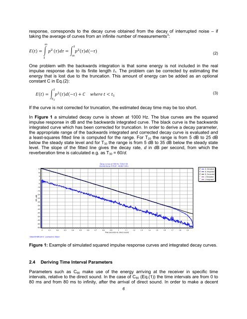In Figure 1 a simulated decay curve is shown at 1000 Hz. The blue curves are the squared impulse response in dB and the backwards integrated curve. The black curve is the backwards integrated curve which has been corrected for truncation. In order to derive a decay parameter, the appropriate range of the backwards integrated and corrected decay curve is evaluated and a least-squares fitted line is computed for the range. For T 20 the range is from 5 dB to 25 dB below the steady state level and for T 30 the range is from 5 dB to 35 dB below the steady state level. The slope of the fitted line gives the decay rate, d in dB per second, from which the reverberation time is calculated e.g. as T 30 = 60/d. Decay curves at 1000 Hz, T(30)=1,90 Zoomed decay T(15,67, -46,26)=1,90 s 15 10 5 0 gfedcb gfedcb gfedcb gfedc gfedc E, Simulated E, Integrated E, Corrected I, Simulated I, Integrated -5 -10 -15 -20 -25 -30 -35 -40 -45 -50 -55 -60 -65 0 0,1 0,2 0,3 0,4 0,5 0,6 0,7 0,8 0,9 1 1,1 Time (seconds rel. direct sound) 1,2 1,3 1,4 1,5 1,6 1,7 1,8 1,9 <strong>Odeon</strong>©1985-2013 Licensed to: <strong>Odeon</strong> Figure 1: Example of simulated squared impulse response curves and integrated decay curves. 2.4 Deriving Time Interval Parameters Parameters such as C 80 make use of the energy arriving at the receiver in specific time intervals, relative to the direct sound. In the case of C 80 (Eq.(1)) the time intervals are from 0 to 80 ms and from 80 ms to infinity, after the arrival of direct sound. In order to make a decent 6
prediction of C 80 it is important that the onset time is well defined. When the source is visible from the receiver this is not a problem as the onset time can be derived from source and receiver position and even in slightly coupled spaces this may be precise enough. Measured time interval parameters may not be precisely derived if calculated directly from the filtered response, because filters create delay and smear the response in time. This can be particularly significant for the lower frequency octave bands where the filters are “long”. In order to bypass this filter problem, ISO 3382-1 suggest the “Window-before-filtering” approach which is the method implemented in ODEON. First the onset time is estimated from the broad band impulse response. In order to estimate the energy arriving for example during the first 80 ms, the first 80 ms of the broad band response arriving after the onset time is gated and octave band filtered afterwards. This creates a filtered response which is longer than the original broad band response in order to include the filter tail. Then the energy of the gated filtered response is counted including the tail of the filter, taking into account most of the smeared energy. Note that the C 80 parameter may not make sense in a space where receiver and source positions are strongly decoupled as the build-up of the impulse response may take considerably longer than the 80 milliseconds. 3 IMPULSE RESPONSE MEASUREMENTS In contrast to impulse response simulations (Sec.2), measurements may be considered accurate in a broader frequency area, due to the actual representation of wave phenomena (interaction due to phase shifts, diffraction etc.). Input data such as absorption and scattering coefficients are inherent and the room geometry is fully included by definition. On the other hand, a group of limitations, such as imperfect omni-directional sources, presence of background noise and distortion due to the filtering required impose errors in the final results. Table 4 summarizes the facts associated with existing measurement and simulation processes. The main issues for measurements are those related to the sound source and the background noise. For the simulations the most important issues are the material data and the approximation of the wave phenomena. Table 4: Facts associated to measurements and simulations. Facts Measurements Simulations Room geometry Fully included by definition Approximated Alteration of room geometry Difficult Easy Wave phenomena (phase information, diffraction) Wall properties Fully included – inherent in the real sound field Fully included – inherent in the real room Approximated with varying accuracy Absorption - scattering coefficients have to measured or assumed, with limited accuracy 7
Page 1 and 2: Toronto, Canada International Sympo
Page 3 and 4: Table 1: Room Acoustic Parameters i
Page 5: scattering coefficients have been a
Page 9 and 10: SPL(dB) can be some influence from
Page 11 and 12: is used for separating multiple imp
Page 13 and 14: p x E-1 Impulse response recordings
Page 15 and 16: SPL / Noise (dB) an indicator wheth
Page 17 and 18: Ts (ms) SPL (dB) Statistics Active
Page 19 and 20: 4.3 Different excitation stimuli Fo
Page 21 and 22: R3 at 4,55 m R2 at 6,84 m R5 at 8,9
Page 23 and 24: In Figure 16 measured and simulated
Page 25 and 26: 6 CONCLUSIONS It is possible to mak

paper - Odeon

Create successful ePaper yourself

Delete template?

Save as template?