Chapter 9: Introduction to Hypothesis Testing

382 CHAPTER 9 • INTRODUCTION TO HYPOTHESIS TESTING
Critical Value
The value corresponding to a
significance level that determines
those test statistics that lead to
rejecting the null hypothesis and
those that lead to a decision not to
reject the null hypothesis.
CHAPTER OUTCOME #4
Business
Application
The decision maker carrying out the test specifies the significance level, . The value
of is determined based on the costs involved in committing a Type I error. If making a
Type I error is costly, we will want the probability of a Type I error to be small. If a Type I
error is less costly, then we can allow a higher probability of a Type I error.
However, in determining , we must also take into account the probability of making
a Type II error, which is given the symbol (beta). The two error probabilities, and ,
are inversely related. 2 That is, if we reduce , then will increase. Thus, in setting , you
must consider both sides of the issue.
Calculating the specific dollar costs associated with making Type I and Type II errors
is often difficult and may require a subjective management decision. Therefore, any two
managers might well arrive at different alpha levels. However, in the end, the choice for
alpha must reflect the decision maker’s best estimate of the costs of these two errors. 3
Having chosen a significance level , the decision maker then must calculate the
corresponding cutoff point, which is called a critical value.
Hypothesis Test for , Known
Calculating Critical Values To calculate critical values corresponding to a chosen , we
need to know the sampling distribution of the sample mean x. If our sampling conditions
satisfy the Central Limit Theorem requirements or if the population is normally distributed
and we know the population standard deviation , then the sampling distribution of x is
normal with mean equal to the population mean μ and standard deviation / n. 4 With this
information we can calculate a critical z-value, called z
, or a critical x-value, called x .
We illustrate both calculations in the Morgan Lane Real Estate example.
MORGAN LANE REAL ESTATE (CONTINUED) Suppose the managing partners decide they
are willing to incur a 0.10 probability of committing a Type I error. Assume also that the
population standard deviation, , for closing is 3 days and the sample size is 64 homes.
Given that the sample size is large (n 30) and that the population standard deviation is
known (3 days), we can state the critical value in two ways. First, we can establish the
critical value as a z-value.
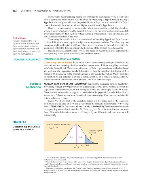
Figure 9.3 shows that if the rejection region on the upper end of the sampling
distribution has an area of 0.10, the z-value from the standard normal table (or by using
Excel’s NORMSINV function or Minitab’s Calc Probability Distributions command)
corresponding to the critical value is 1.28. Thus, z 0.10
1.28. If the sample mean lies more
than 1.28 standard deviations above 25 days, H 0
should be rejected; otherwise we will
not reject H 0
.
FIGURE 9.3
Determining the Critical
Value as a z-Value
From the standard normal table
z 0.10 = 1.28
0.5 0.4
Rejection region
α = 0.10
0
μ = 25
z 0.10 = 1.28
z
2 The sum of alpha and beta may coincidently equal 1. However, in general, the sum of these two error
probabilities does not equal 1.
3 We will discuss Type II errors more fully later in this chapter. Contrary to the Type I situation in which we
specify the desired alpha level, beta is computed based on certain assumptions. Methods for computing beta are
shown in Section 9.3.
4 For many population distributions, the Central Limit Theorem applies for sample sizes as small as 4 or 5.
Sample sizes n 30 assure us that the sampling distribution will be approximately normal regardless of population
distribution.