Chapter 9: Introduction to Hypothesis Testing
Chapter 9: Introduction to Hypothesis Testing
Chapter 9: Introduction to Hypothesis Testing

You also want an ePaper? Increase the reach of your titles
YUMPU automatically turns print PDFs into web optimized ePapers that Google loves.
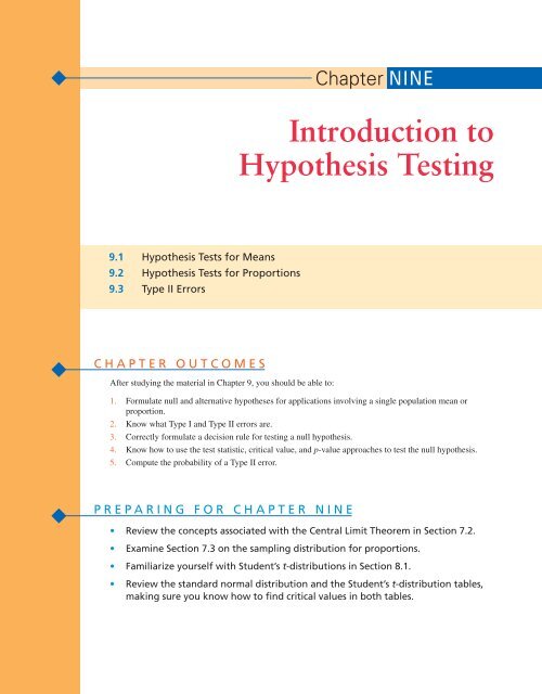
<strong>Chapter</strong> NINE<br />
<strong>Introduction</strong> <strong>to</strong><br />
<strong>Hypothesis</strong> <strong>Testing</strong><br />
9.1 <strong>Hypothesis</strong> Tests for Means<br />
9.2 <strong>Hypothesis</strong> Tests for Proportions<br />
9.3 Type II Errors<br />
CHAPTER OUTCOMES<br />
After studying the material in <strong>Chapter</strong> 9, you should be able <strong>to</strong>:<br />
1. Formulate null and alternative hypotheses for applications involving a single population mean or<br />
proportion.<br />
2. Know what Type I and Type II errors are.<br />
3. Correctly formulate a decision rule for testing a null hypothesis.<br />
4. Know how <strong>to</strong> use the test statistic, critical value, and p-value approaches <strong>to</strong> test the null hypothesis.<br />
5. Compute the probability of a Type II error.<br />
PREPARING FOR CHAPTER NINE<br />
• Review the concepts associated with the Central Limit Theorem in Section 7.2.<br />
• Examine Section 7.3 on the sampling distribution for proportions.<br />
• Familiarize yourself with Student’s t-distributions in Section 8.1.<br />
• Review the standard normal distribution and the Student’s t-distribution tables,<br />
making sure you know how <strong>to</strong> find critical values in both tables.
376 CHAPTER 9 • INTRODUCTION TO HYPOTHESIS TESTING<br />
W HY Y OU N EED T O K NOW<br />
As a business decision maker, you will encounter many<br />
applications that will require you <strong>to</strong> estimate a population<br />
parameter. <strong>Chapter</strong> 8 introduced statistical estimation and<br />
included many examples. Estimating a population parameter<br />
based on a sample statistic is a component of business<br />
statistics called statistical inference. An important component<br />
of statistical inference is hypothesis testing. In<br />
hypothesis testing, we begin with some belief regarding<br />
what the value of a population parameter is, or should be.<br />
We then use sample data <strong>to</strong> either refute or support the<br />
initial belief.<br />
For example, suppose the Coca-Cola plant in Tampa,<br />
Florida, produces approximately 400,000 cans of Coke<br />
products daily. Each can is supposed <strong>to</strong> contain 12 fluid<br />
ounces. However, like all processes, the au<strong>to</strong>mated filling<br />
machine is subject <strong>to</strong> variation and each can will contain<br />
either slightly more or less than the 12-ounce target. The<br />
important thing is that the mean fill is 12 fluid ounces.<br />
Every two hours, the plant quality manager selects a random<br />
sample of cans and computes the sample mean. His<br />
initial belief is that the filling process is providing an average<br />
fill of 12 ounces. This is his hypothesis. If the sample<br />
mean is “close” <strong>to</strong> 12 ounces, then the sample data would<br />
tend <strong>to</strong> support the hypothesis and the machine would be<br />
allowed <strong>to</strong> continue filling cans. However, if the sample<br />
mean is “significantly” higher or lower than 12 ounces,<br />
the data would refute the hypothesis and the machine<br />
would be s<strong>to</strong>pped and adjusted.<br />
<strong>Hypothesis</strong> testing is performed regularly in many<br />
industries. Companies in the pharmaceutical industry must<br />
perform many hypothesis tests on new drug products<br />
before they are deemed <strong>to</strong> be safe and effective by the<br />
federal Food and Drug Administration (FDA). In these<br />
instances, the drug is hypothesized <strong>to</strong> be both unsafe and<br />
ineffective. Then, if the sample results from the studies<br />
performed provide “significant” evidence <strong>to</strong> the contrary,<br />
the FDA will allow the company <strong>to</strong> market the drug.<br />
<strong>Hypothesis</strong> testing is the basis of the legal system in<br />
which judges and juries hear evidence in court cases. In a<br />
criminal case, the hypothesis in the American legal system<br />
is that the defendant is innocent. Based upon the <strong>to</strong>tality<br />
of the evidence presented in the trial, if the jury concludes<br />
that “beyond a reasonable doubt” the defendant committed<br />
the crime, the hypothesis of innocence will be rejected<br />
and the defendant will be found guilty. If the evidence is<br />
not strong enough, the defendant will be judged not guilty.<br />
<strong>Hypothesis</strong> testing is a major part of business statistics.<br />
<strong>Chapter</strong> 9 introduces the fundamentals involved in<br />
conducting hypothesis tests. Many of the remaining chapters<br />
in this text will introduce additional hypothesis-testing<br />
techniques, so you need <strong>to</strong> gain a solid understanding of<br />
concepts presented in this chapter.<br />
Null <strong>Hypothesis</strong><br />
The statement about the<br />
population parameter that will be<br />
tested. The null hypothesis will<br />
be rejected only if the sample data<br />
provide substantial contradic<strong>to</strong>ry<br />
evidence.<br />
Alternative <strong>Hypothesis</strong><br />
The hypothesis that includes all<br />
population values not included in<br />
the null hypothesis. The alternative<br />
hypothesis is deemed <strong>to</strong> be true if<br />
the null hypothesis is rejected.<br />
9.1 <strong>Hypothesis</strong> Tests for Means<br />
By now you know that information contained in a sample is subject <strong>to</strong> sampling error. The<br />
sample mean will almost certainly not equal the population mean. Therefore, in situations in<br />
which you need <strong>to</strong> test a claim about a population mean by using the sample mean, you can’t<br />
simply compare the sample mean <strong>to</strong> the claim and reject the claim if x and the claim are different.<br />
Instead, you need a testing procedure that incorporates the potential for sampling error.<br />
Statistical hypothesis testing provides managers with a structured analytical method for<br />
making decisions of this type. It lets them make decisions in such a way that the probability<br />
of decision errors can be controlled, or at least measured. Even though statistical hypothesis<br />
testing does not eliminate the uncertainty in the managerial environment, the techniques<br />
involved often allow managers <strong>to</strong> identify and control the level of uncertainty.<br />
The techniques presented in this chapter assume the data are selected using an appropriate<br />
statistical sampling process and that the data are interval or ratio level. In short, we<br />
assume we are working with good data.<br />
Formulating the Hypotheses<br />
Null and Alternative Hypotheses In hypothesis testing, two hypotheses are formulated.<br />
One is the null hypothesis. The null hypothesis is represented by H 0<br />
and contains an<br />
equality sign, such as “,” “,” or “.” The second hypothesis is the alternative hypothesis<br />
(represented by H A<br />
). Based on the sample data, we either reject H 0<br />
or we do not<br />
reject H 0<br />
.<br />
Correctly specifying the null and alternative hypotheses is important. If done incorrectly,<br />
the results obtained from the hypothesis test may be misleading. Unfortunately, how you
CHAPTER 9 • INTRODUCTION TO HYPOTHESIS TESTING 377<br />
should formulate the null and alternative hypotheses is not always obvious. As you gain<br />
experience with hypothesis-testing applications, the process becomes easier. To help you get<br />
started, we have developed some guidelines for specifying the null and alternative hypotheses.<br />
The major point <strong>to</strong> remember is the “benefit of the doubt” goes <strong>to</strong> the null hypothesis.<br />
Only significant differences will lead <strong>to</strong> rejecting the null hypothesis.<br />
<strong>Testing</strong> the Status Quo In many cases, you will be interested in whether a situation has<br />
changed. We refer <strong>to</strong> this as testing the status quo, and this is a common application of<br />
hypothesis testing. For example, the Kellogg Company makes many food products, including<br />
a variety of breakfast cereals. At the company’s Battle Creek, Michigan, plant, Frosted<br />
Mini-Wheats are produced and packaged for distribution around the world. If the packaging<br />
process is working properly, the mean fill per box is 16 ounces. Every hour quality<br />
analysts at the plant select a random sample of filled boxes and measure their contents.<br />
They use the sample data <strong>to</strong> test the following null and alternative hypotheses:<br />
H 0<br />
: 16 ounces (status quo)<br />
H A<br />
: 16 ounces<br />
The null hypothesis is reasonable because the line supervisor would assume the<br />
process is operating correctly before starting production. As long as the sample mean is<br />
“reasonably” close <strong>to</strong> 16 ounces, the analysts will assume the filling process is working<br />
properly. Only when the sample mean is seen <strong>to</strong> be <strong>to</strong>o large or <strong>to</strong>o small will the analysts<br />
reject the null hypothesis (the status quo) and take action <strong>to</strong> identify and fix the problem.<br />
As another example, the Transportation Security Administration (TSA), which is<br />
responsible for screening passengers at U.S. airports, publishes on its Web site the average<br />
waiting times for cus<strong>to</strong>mers <strong>to</strong> pass through security. For example, on Mondays between<br />
9:00 and 10:00 A.M., the average waiting time at Atlanta’s Hartsfield International Airport<br />
is supposed <strong>to</strong> be 15 minutes or less. Periodically, TSA staff will select a random sample of<br />
passengers during this time slot and measure their actual wait times. These sample data<br />
will be used <strong>to</strong> test the following null and alternative hypotheses:<br />
H 0<br />
: 15 minutes (status quo)<br />
H A<br />
: 15 minutes<br />
Only if the sample mean wait time is “substantially” greater than 15 minutes will TSA<br />
employees reject the null hypothesis and conclude there is a problem with staffing levels.<br />
Otherwise, they will assume that the 15-minute standard (the status quo) is being met and<br />
no action will be taken.<br />
Research <strong>Hypothesis</strong><br />
The hypothesis the decision maker<br />
attempts <strong>to</strong> demonstrate <strong>to</strong> be true.<br />
Because this is the hypothesis<br />
deemed <strong>to</strong> be the most important<br />
<strong>to</strong> the decision maker, it will be<br />
declared true only if the sample<br />
data strongly indicates that it is true.<br />
<strong>Testing</strong> a Research <strong>Hypothesis</strong> Many business and scientific applications involve<br />
research applications. For example, companies such as Intel, Procter & Gamble, Dell<br />
Computers, Pfizer, and 3M continually introduce new and improved products. However,<br />
before introducing a new product, the companies want <strong>to</strong> be sure that the new product is superior<br />
<strong>to</strong> the original. In the case of drug companies like Pfizer, the government requires them <strong>to</strong><br />
show their product is both safe and effective. Because statistical evidence is needed <strong>to</strong> indicate<br />
that the new product is effective, the default position (or null hypothesis) is it is no better than<br />
the original (or in the case of a drug, it is unsafe and ineffective.) The burden of proof is placed<br />
on the new product and the alternative hypothesis is formulated as the research hypothesis.<br />
For example, suppose the Goodyear Tire and Rubber Company has a new tread design<br />
that its engineers claim will outlast its competi<strong>to</strong>r’s leading tire. The competi<strong>to</strong>r’s tire<br />
has been demonstrated <strong>to</strong> provide an average of 60,000 miles of use. Thus the research<br />
hypothesis for Goodyear is that its tire is superior, meaning that it will last more than<br />
60,000 miles. The research hypothesis becomes the alternative hypothesis:<br />
H 0<br />
: 60,000<br />
H A<br />
: 60,000 (research hypothesis)<br />
The burden of proof is on Goodyear. Only if the sample data show a sample mean that<br />
is “substantially” larger than 60,000 miles will the null hypothesis be rejected and<br />
Goodyear’s position be affirmed.
378 CHAPTER 9 • INTRODUCTION TO HYPOTHESIS TESTING<br />
In another example, suppose the Agri-Seed Company has developed a new fertilizer for<br />
commercial farming. Agri-Seed would introduce this product on the market only if it provides<br />
yields superior <strong>to</strong> its current fertilizer product. Experience shows that when the current fertilizer<br />
is used <strong>to</strong> grow sugar beets, a mean yield of 30 <strong>to</strong>ns per acre is expected. To test the new<br />
fertilizer, Agri-Seed researchers will set up the following null and alternative hypotheses:<br />
H 0<br />
: 30 <strong>to</strong>ns<br />
H A<br />
: 30 <strong>to</strong>ns (research hypothesis)<br />
The alternative hypothesis is the research hypothesis. If the null hypothesis is rejected, then<br />
Agri-Seed will have statistical evidence <strong>to</strong> show that the new fertilizer is superior <strong>to</strong> the<br />
existing product.<br />
<strong>Testing</strong> a Claim About the Population Analyzing claims using hypothesis tests can be<br />
complicated because the benefit of the doubt goes <strong>to</strong> the null hypothesis. Sometimes you<br />
will want <strong>to</strong> give the benefit of the doubt <strong>to</strong> the claim, but in other instances you will be<br />
skeptical about the claim and will want <strong>to</strong> place the burden of proof on the claim. For consistency<br />
purposes, the rule adopted in this text is that if the claim contains the equality, the<br />
claim goes in the null. If the claim does not contain the equality, it goes in the alternative.<br />
A recent radio commercial has stated the average waiting time at a medical clinic is<br />
less than 15 minutes. A claim like this can be tested using hypothesis testing. The null and<br />
alternative hypotheses should be formulated such that one contains the claim and the other<br />
reflects the opposite position. Since the claim does not contain the equality ( 15), the<br />
claim should be the alternative hypothesis. The appropriate null and alternative hypotheses<br />
are, then, as follows:<br />
H 0<br />
: 15<br />
H A<br />
: 15 (claim)<br />
In cases like this where the claim corresponds <strong>to</strong> the alternative hypothesis, the burden<br />
of proof is on the medical clinic. If the sample mean is “substantially” less than 15 minutes,<br />
the null hypothesis would be rejected and the alternative hypothesis (and the claim)<br />
would be accepted. Otherwise, the null hypothesis would not be rejected and the claim<br />
could not be accepted.<br />
SUMMARY Formulating the Null and Alternative Hypotheses<br />
1. The null and alternative hypotheses must be stated<br />
in terms of the population of interest (e.g., , ,<br />
or ).<br />
2. If the application involves a test of the status quo,<br />
the status quo forms the null hypothesis and the<br />
burden of proof is <strong>to</strong> show that the status quo has<br />
changed.<br />
3. If the application involves a research issue, the research<br />
hypothesis forms the alternative hypothesis.<br />
4. If a claim has been made about the population parameter,<br />
the decision maker must determine if he or she is<br />
inclined <strong>to</strong> agree with the claim before gathering any<br />
data. If so, the claim establishes the null hypothesis;<br />
otherwise, it forms the alternative hypothesis.<br />
EXAMPLE 9-1 Formulating the Null and Alternative Hypotheses<br />
CHAPTER OUTCOMES #1<br />
TRY PROBLEM 9.13<br />
Student Work Hours In <strong>to</strong>day’s economy, university students often work many<br />
hours <strong>to</strong> help pay for the high costs of a college education. Suppose a university in the<br />
Midwest is considering changing its class schedule <strong>to</strong> accommodate students working<br />
long hours. The registrar has stated a change is needed because the mean number of
CHAPTER 9 • INTRODUCTION TO HYPOTHESIS TESTING 379<br />
hours worked by undergraduate students at the university is more than 20 per week. The<br />
following steps can be taken <strong>to</strong> establish the appropriate null and alternative hypotheses:<br />
Step 1 Determine the population parameter of interest.<br />
In this case, the population parameter of interest is the mean hours<br />
worked, μ. The null and alternative hypotheses must be stated in terms of<br />
the population parameter.<br />
Step 2 Determine whether the application involves a test of the status quo,<br />
a research application, or a claim about the population parameter.<br />
In this case, the registrar has made a claim stating that the mean hours<br />
worked “is more than 20” per week. Because changing the class scheduling<br />
system would be expensive and time-consuming, the assumption is<br />
made that the number of hours worked is less than or equal <strong>to</strong> 20. Thus,<br />
the burden of proof is placed on the registrar <strong>to</strong> justify her claim that the<br />
mean is greater than 20 hours.<br />
Step 3 Formulate the null and alternative hypotheses.<br />
Keep in mind that the equality goes in the null hypothesis.<br />
H 0<br />
: 20 hours<br />
H A<br />
: 20 hours (claim)<br />
Example 9-2 illustrates another example of how the null and alternative hypotheses<br />
are formulated.<br />
EXAMPLE 9-2<br />
Formulating the Null and Alternative Hypotheses<br />
TRY PROBLEM 9.14<br />
Boulder Pota<strong>to</strong> Company The Boulder Pota<strong>to</strong> Company produces several snack and<br />
food products that are sold in food s<strong>to</strong>res throughout Colorado and Arizona. The company<br />
uses an au<strong>to</strong>matic filling machine <strong>to</strong> fill the sacks with the desired weight. For instance,<br />
when the company is running pota<strong>to</strong> chips on the fill line, the machine is set <strong>to</strong> fill the sacks<br />
with 20 ounces. Thus, if the machine is working properly, the mean fill will be 20 ounces.<br />
Each hour, a sample of sacks is collected and weighed, and the technicians determine<br />
whether the machine is still operating correctly or whether it needs adjustment. The following<br />
steps can be used <strong>to</strong> establish the null and alternative hypotheses <strong>to</strong> be tested.<br />
Step 1 Determine the population parameter of interest.<br />
In this case, the population parameter of interest is the mean weight per<br />
sack, .<br />
Step 2 Determine whether the application involves a claim about the population<br />
parameter, a research application, or a test of the status quo.<br />
The status quo is that the machine is filling the sacks with the proper<br />
amount, which is 20 ounces. We will believe this <strong>to</strong> be true unless we<br />
find evidence <strong>to</strong> suggest otherwise. If such evidence exists, then the filling<br />
process needs <strong>to</strong> be adjusted.<br />
Step 3 Formulate the null and alternative hypotheses.<br />
Keep in mind that the equality goes in the null hypothesis.<br />
The null and alternative hypotheses are<br />
H 0<br />
: 20 ounces (status quo)<br />
H A<br />
: 20 ounces
380 CHAPTER 9 • INTRODUCTION TO HYPOTHESIS TESTING<br />
FIGURE 9.1<br />
State of Nature<br />
The Relationship<br />
Between Decisions and<br />
States of Nature<br />
Decision<br />
Conclude Null True<br />
(Don’t reject H 0 )<br />
Conclude Null False<br />
(Reject H 0 )<br />
Null <strong>Hypothesis</strong> True Null <strong>Hypothesis</strong> False<br />
Correct Decision<br />
Type II Error<br />
Type I Error<br />
Correct Decision<br />
Type I Error<br />
Rejecting the null hypothesis when<br />
it is, in fact, true.<br />
Type II Error<br />
Failing <strong>to</strong> reject the null hypothesis<br />
when it is, in fact, false.<br />
CHAPTER OUTCOME #2<br />
Business<br />
Application<br />
Types of Statistical Errors Because of the potential for extreme sampling error, two<br />
possible errors can occur when a hypothesis is tested: Type I and Type II errors. These<br />
errors show the relationship between what actually exists (a state of nature) and the decision<br />
made based on the sample information.<br />
Figure 9.1 shows the possible actions and states of nature associated with any hypothesis-testing<br />
application. As you can see, there are three possible outcomes: no error (correct<br />
decision), Type I error, and Type II error. Only one of these outcomes will occur for a<br />
hypothesis test. From Figure 9.1, if the null hypothesis is true and an error is made, it must<br />
be a Type I error. On the other hand, if the null hypothesis is false and an error is made, it<br />
must be a Type II error.<br />
Many statisticians argue that you should never use the phrase “accept the null<br />
hypothesis.” Instead you should use “do not reject the null hypothesis.” Thus, the only two<br />
hypothesis-testing decisions would be reject H 0<br />
or “do not reject H 0<br />
.” This is why in a jury<br />
verdict <strong>to</strong> acquit a defendant, the verdict is “not guilty” rather than innocent. Just because<br />
the evidence is insufficient <strong>to</strong> convict does not necessarily mean that the defendant is<br />
innocent.<br />
This thinking is appropriate when hypothesis testing is employed in situations in<br />
which some future action is not dependent on the results of the hypothesis test. However,<br />
in most business applications, the purpose of the hypothesis test is <strong>to</strong> direct the decision<br />
maker <strong>to</strong> take one action or another, based on the test results. So, in this text, when hypothesis<br />
testing is applied <strong>to</strong> decision-making situations, not rejecting the null hypothesis is<br />
essentially the same as accepting it. 1<br />
MORGAN LANE REAL ESTATE COMPANY The Morgan Lane Real Estate Company has<br />
offices in and around the Napa Valley in the northern California wine country. The real<br />
estate market in this area has been “hot” for a number of years and homes commonly sell<br />
above the asking price very quickly. Once a buyer and seller agree <strong>to</strong> terms on a home, the<br />
closing process (appraisal, inspection, loan application, etc.) begins. The standard time for<br />
closings in the Napa area is no more than 25 days. The managing partner at Morgan Lane<br />
wishes <strong>to</strong> test whether her agency’s closings are meeting this standard. Treating the<br />
25 days as the status quo, the null and alternative hypotheses <strong>to</strong> be tested are<br />
H 0<br />
: 25 days (status quo)<br />
H A<br />
: 25 days<br />
She will select a random sample of home sales closed by Morgan Lane agents. In this<br />
application, a Type I error would occur if the sample data lead the manager <strong>to</strong> conclude<br />
that the mean closing time exceeds 25 days (H 0<br />
is rejected) when in fact 25 days. If a<br />
Type I error occurred, the manager would needlessly spend time and resources trying <strong>to</strong><br />
speed up a process that already meets the industry standards.<br />
Alternatively, a Type II error would occur if the sample evidence leads the manager <strong>to</strong><br />
incorrectly conclude that 25 days (H 0<br />
is not rejected) when the mean closing time<br />
1 Whichever language you use, you should make an effort <strong>to</strong> understand both arguments and make an<br />
informed choice. If your instruc<strong>to</strong>r requests that you reference the action in a particular way, it would behoove<br />
you <strong>to</strong> follow the instructions. Having gone through this process ourselves, we prefer <strong>to</strong> state the choice as<br />
“don’t reject the null hypothesis.” This terminology will be used throughout this text.
CHAPTER 9 • INTRODUCTION TO HYPOTHESIS TESTING 381<br />
exceeds 25 days. Now the manager would take no action <strong>to</strong> improve closing times at<br />
Morgan Lane when changes are needed <strong>to</strong> improve cus<strong>to</strong>mer service.<br />
CHAPTER OUTCOME #3<br />
Significance Level and Critical Value<br />
The objective of a hypothesis test is <strong>to</strong> use sample information <strong>to</strong> decide whether <strong>to</strong> reject<br />
the null hypothesis about a population parameter. How do decision makers determine<br />
whether the sample information supports or refutes the null hypothesis? The answer <strong>to</strong> this<br />
question is the key <strong>to</strong> understanding statistical hypothesis testing.<br />
In hypotheses tests for a single population mean, the sample mean, x, is used <strong>to</strong> test<br />
the hypotheses under consideration. Depending on how the null and alternative hypotheses<br />
are formulated, certain values of x will tend <strong>to</strong> support the null hypothesis, whereas other<br />
values will appear <strong>to</strong> contradict it. In the Morgan Lane example, the null and alternative<br />
hypotheses were formulated as<br />
H 0<br />
: 25 days<br />
H A<br />
: 25 days<br />
Values of x less than or equal <strong>to</strong> 25 days would tend <strong>to</strong> support the null hypothesis. By<br />
contrast, values of x greater than 25 days would tend <strong>to</strong> refute the null hypothesis. The<br />
larger the value of x, the greater the evidence that the null hypothesis should be rejected.<br />
However, because we expect some sampling error, do we want <strong>to</strong> reject H 0<br />
for any value<br />
of x that is greater than 25 days? Probably not. But should we reject H 0<br />
if x 26 days,<br />
or x 30 days, or x 35 days? At what point do we s<strong>to</strong>p attributing the result <strong>to</strong> sampling<br />
error?<br />
In order <strong>to</strong> perform the hypothesis test, we need <strong>to</strong> select a cu<strong>to</strong>ff point that is the demarcation<br />
between rejecting and not rejecting the null hypothesis. Our decision rule for the<br />
Morgan Lane application is then<br />
If x cu<strong>to</strong>ff, reject H0 .<br />
If x cu<strong>to</strong>ff, do not reject H 0<br />
.<br />
Significance Level<br />
The maximum allowable<br />
probability of committing a Type I<br />
statistical error. The probability is<br />
denoted by the symbol .<br />
If x is greater than the cu<strong>to</strong>ff, we will reject H 0<br />
and conclude that the average closing time<br />
does exceed 25 days. If x is less than or equal <strong>to</strong> the cu<strong>to</strong>ff, we will not reject H 0<br />
; in this<br />
case our test does not give sufficient evidence that the closing time exceeds 25 days.<br />
Recall from the Central Limit Theorem (see <strong>Chapter</strong> 7) that, for large samples, the<br />
distribution of the possible sample means is approximately normal, with a center at the<br />
population mean . The null hypothesis in our example is 25 days. Figure 9.2 shows<br />
the sampling distribution for x assuming that 25. The shaded region on the right is<br />
called the rejection region. The area of the rejection region gives the probability of getting<br />
an x larger than the cu<strong>to</strong>ff when μ is really 25, so it is the probability of making a Type I<br />
statistical error. This probability is called the significance level of the test and is given the<br />
symbol (alpha).<br />
FIGURE 9.2<br />
Sampling Distribution<br />
of x for Morgan Lane<br />
Sampling Distribution<br />
Do not reject H 0<br />
Probability of<br />
committing a Type I<br />
error = α<br />
μ = 25<br />
x<br />
Cu<strong>to</strong>ff Reject H 0
382 CHAPTER 9 • INTRODUCTION TO HYPOTHESIS TESTING<br />
Critical Value<br />
The value corresponding <strong>to</strong> a<br />
significance level that determines<br />
those test statistics that lead <strong>to</strong><br />
rejecting the null hypothesis and<br />
those that lead <strong>to</strong> a decision not <strong>to</strong><br />
reject the null hypothesis.<br />
CHAPTER OUTCOME #4<br />
Business<br />
Application<br />
The decision maker carrying out the test specifies the significance level, . The value<br />
of is determined based on the costs involved in committing a Type I error. If making a<br />
Type I error is costly, we will want the probability of a Type I error <strong>to</strong> be small. If a Type I<br />
error is less costly, then we can allow a higher probability of a Type I error.<br />
However, in determining , we must also take in<strong>to</strong> account the probability of making<br />
a Type II error, which is given the symbol (beta). The two error probabilities, and ,<br />
are inversely related. 2 That is, if we reduce , then will increase. Thus, in setting , you<br />
must consider both sides of the issue.<br />
Calculating the specific dollar costs associated with making Type I and Type II errors<br />
is often difficult and may require a subjective management decision. Therefore, any two<br />
managers might well arrive at different alpha levels. However, in the end, the choice for<br />
alpha must reflect the decision maker’s best estimate of the costs of these two errors. 3<br />
Having chosen a significance level , the decision maker then must calculate the<br />
corresponding cu<strong>to</strong>ff point, which is called a critical value.<br />
<strong>Hypothesis</strong> Test for , Known<br />
Calculating Critical Values To calculate critical values corresponding <strong>to</strong> a chosen , we<br />
need <strong>to</strong> know the sampling distribution of the sample mean x. If our sampling conditions<br />
satisfy the Central Limit Theorem requirements or if the population is normally distributed<br />
and we know the population standard deviation , then the sampling distribution of x is<br />
normal with mean equal <strong>to</strong> the population mean μ and standard deviation / n. 4 With this<br />
information we can calculate a critical z-value, called z <br />
, or a critical x-value, called x .<br />
We illustrate both calculations in the Morgan Lane Real Estate example.<br />
MORGAN LANE REAL ESTATE (CONTINUED) Suppose the managing partners decide they<br />
are willing <strong>to</strong> incur a 0.10 probability of committing a Type I error. Assume also that the<br />
population standard deviation, , for closing is 3 days and the sample size is 64 homes.<br />
Given that the sample size is large (n 30) and that the population standard deviation is<br />
known (3 days), we can state the critical value in two ways. First, we can establish the<br />
critical value as a z-value.<br />
Figure 9.3 shows that if the rejection region on the upper end of the sampling<br />
distribution has an area of 0.10, the z-value from the standard normal table (or by using<br />
Excel’s NORMSINV function or Minitab’s Calc Probability Distributions command)<br />
corresponding <strong>to</strong> the critical value is 1.28. Thus, z 0.10<br />
1.28. If the sample mean lies more<br />
than 1.28 standard deviations above 25 days, H 0<br />
should be rejected; otherwise we will<br />
not reject H 0<br />
.<br />
FIGURE 9.3<br />
Determining the Critical<br />
Value as a z-Value<br />
From the standard normal table<br />
z 0.10 = 1.28<br />
0.5 0.4<br />
Rejection region<br />
α = 0.10<br />
0<br />
μ = 25<br />
z 0.10 = 1.28<br />
z<br />
2 The sum of alpha and beta may coincidently equal 1. However, in general, the sum of these two error<br />
probabilities does not equal 1.<br />
3 We will discuss Type II errors more fully later in this chapter. Contrary <strong>to</strong> the Type I situation in which we<br />
specify the desired alpha level, beta is computed based on certain assumptions. Methods for computing beta are<br />
shown in Section 9.3.<br />
4 For many population distributions, the Central Limit Theorem applies for sample sizes as small as 4 or 5.<br />
Sample sizes n 30 assure us that the sampling distribution will be approximately normal regardless of population<br />
distribution.
CHAPTER 9 • INTRODUCTION TO HYPOTHESIS TESTING 383<br />
FIGURE 9.4<br />
Determining the Critical<br />
Value as an x-Value,<br />
Morgan Lane Example<br />
σ<br />
σ x = =<br />
n<br />
3<br />
64<br />
0.5 0.4<br />
Rejection region<br />
α = 0.10<br />
0<br />
μ = 25<br />
z 0.10 = 1.28<br />
x 0.10 = 25.48<br />
z<br />
Solving for x α<br />
x 0.10 = μ + z 0.10<br />
x 0.10 = 25.48<br />
σ<br />
n<br />
= 25 + 1.28<br />
3<br />
64<br />
We can also express the critical value in the same units as the sample mean. In the<br />
Morgan Lane example, we can calculate a critical x value, x , so that if x is greater than the<br />
critical value, we should reject H 0<br />
. If x is less than or equal <strong>to</strong> x , we should not reject H 0<br />
.<br />
Equation 9.1 shows how x is computed. Figure 9.4 illustrates the use of Equation 9.1 for<br />
computing the critical value, .<br />
x <br />
x <br />
for <strong>Hypothesis</strong> Tests, Known<br />
x<br />
<br />
z<br />
<br />
<br />
n<br />
(9.1)<br />
where:<br />
Hypothesized value for the population mean<br />
z <br />
Critical value from the standard normal distribution<br />
Population standard deviation<br />
n Sample size<br />
Applying Equation 9.1, we determine the value for<br />
as follows:<br />
Also refer <strong>to</strong> Figure 9.4 for a graphical illustration showing how<br />
x<br />
x<br />
x<br />
<br />
010 .<br />
010 .<br />
<br />
<br />
z<br />
n<br />
25 1.<br />
28 3 64<br />
25. 48 days<br />
is determined.<br />
If x 25.48 days, H 0<br />
should be rejected and changes made in the process; otherwise,<br />
H 0<br />
should not be rejected and the process should not be changed. Any sample mean<br />
between 25.48 and 25 days would be attributed <strong>to</strong> sampling error, and the null hypothesis<br />
would not be rejected. A sample mean of 25.48 or fewer days will support the null hypothesis.<br />
Decision Rules and Test Statistics To conduct a hypothesis test, you can use three equivalent<br />
approaches. You can calculate a z-value and compare it <strong>to</strong> the critical value, z <br />
.<br />
Alternatively, you can calculate the sample mean, x, and compare it <strong>to</strong> the critical value, x .<br />
Finally, you can use a method called the p-value approach, <strong>to</strong> be discussed later in this<br />
section. It makes no difference which approach you use, each method yields the same<br />
conclusion.<br />
x <br />
x
384 CHAPTER 9 • INTRODUCTION TO HYPOTHESIS TESTING<br />
Suppose x 26 days. How we test the null hypothesis depends on the procedure we<br />
used <strong>to</strong> establish the critical value. First, using the z-value method, we establish the following<br />
decision rule:<br />
Hypotheses<br />
Decision Rule<br />
H 0<br />
: 25 days<br />
H A<br />
: 25 days<br />
0.10<br />
Test Statistic<br />
A function of the sampled<br />
observations that provides a basis<br />
for testing a statistical hypothesis.<br />
where:<br />
If z z 0.10<br />
, reject H 0<br />
.<br />
If z z 0.10<br />
, do not reject H 0<br />
.<br />
z 0.10<br />
1.28<br />
Recall that the number of homes sampled is 64 and the population standard deviation<br />
is assumed known at 3 days. The calculated z-value is called the test statistic.<br />
The z-test statistic is computed using Equation 9.2.<br />
z-Test Statistic for <strong>Hypothesis</strong> Tests for , Known<br />
x<br />
z <br />
<br />
<br />
n<br />
(9.2)<br />
where:<br />
x Sample mean<br />
Hypothesized value for the population mean<br />
Population standard deviation<br />
n Sample size<br />
Given that x 26 days, applying Equation 9.2 we get<br />
Thus, x 26 is 2.67 standard deviations above the hypothesized mean. Because z is<br />
greater than the critical value,<br />
z 2.67 z 0.10<br />
1.28, reject H 0<br />
.<br />
Now we use the second approach, which established (see Figure 9.4) a decision rule,<br />
as follows:<br />
Decision Rule<br />
Then,<br />
x<br />
z 26<br />
25<br />
267 .<br />
3<br />
n<br />
64<br />
If x x 010 .<br />
, reject H 0<br />
;<br />
Otherwise, do not reject H 0<br />
.<br />
If x 25. 48 days, reject H0;<br />
Otherwise, do not reject H 0<br />
.
CHAPTER 9 • INTRODUCTION TO HYPOTHESIS TESTING 385<br />
Then, because<br />
x26 x010 .<br />
25. 48, reject H0.<br />
Note that the two approaches yield the same conclusion, as they always will if you<br />
perform the calculations correctly. We have found that academic applications of hypothesis<br />
testing tend <strong>to</strong> use the z-value method, whereas organizational applications of hypothesis<br />
testing often use the x approach.<br />
You will often come across a different language used <strong>to</strong> express the outcome of a<br />
hypothesis test. For instance, a statement for the hypothesis test just presented would be<br />
“The hypothesis test was significant at an α (or significance level) of 0.10.” This simply<br />
means that the null hypothesis was rejected using a significance level of 0.10.<br />
SUMMARY One-Tailed Test for a <strong>Hypothesis</strong> About a Population Mean, Known<br />
To test the hypothesis, perform the following steps:<br />
1. Specify the population parameter of interest.<br />
2. Formulate the null hypothesis and the alternative<br />
hypothesis in terms of the population mean, .<br />
3. Specify the desired significance level ().<br />
4. Construct the rejection region. (We strongly suggest you<br />
draw a picture showing where in the distribution the<br />
rejection region is located.)<br />
5. Compute the test statistic.<br />
x x<br />
x ∑ or z <br />
n <br />
n<br />
6. Reach a decision. Compare the test statistic with x or z α<br />
.<br />
7. Draw a conclusion regarding the null hypothesis.<br />
EXAMPLE 9-3 One-Tailed <strong>Hypothesis</strong> Test for , Known<br />
TRY PROBLEM 9.3<br />
Providence Heart Institute The Providence Heart Institute in Columbia, South<br />
Carolina, performs many open-heart surgery procedures. Recently, research physicians at<br />
Providence have developed a new heart bypass surgery procedure that they believe will<br />
reduce the average recovery time. The hospital board will not recommend the new procedure<br />
unless there is substantial evidence <strong>to</strong> suggest that it is better than the existing<br />
procedure. Records indicate that the current mean recovery rate for the standard procedure<br />
is 42 days, with a standard deviation of 5 days. To test whether the new procedure<br />
actually results in a lower mean recovery time, the procedure was performed on a random<br />
sample of 36 patients.<br />
Step 1 Specify the population parameter of interest.<br />
We are interested in the mean recovery time, .<br />
Step 2 Formulate the null and alternative hypotheses.<br />
H 0<br />
: 42 (status quo)<br />
H A<br />
: 42<br />
Step 3 Specify the desired significance level ().<br />
The researchers wish <strong>to</strong> test the hypothesis using a 0.05 level of significance.<br />
Step 4 Construct the rejection region.<br />
This will be a one-tailed test, with the rejection region in the<br />
lower (left-hand) tail of the sampling distribution. The critical
386 CHAPTER 9 • INTRODUCTION TO HYPOTHESIS TESTING<br />
FIGURE 9.5<br />
Providence Heart Institute <strong>Hypothesis</strong> Test<br />
σ x =<br />
n<br />
σ<br />
=<br />
5<br />
36<br />
Rejection region<br />
α = 0.05 0.45<br />
0.50<br />
−z 0.05 = –1.645<br />
0<br />
μ = 42<br />
z<br />
value is z 0.05<br />
1.645. Therefore, the decision rule becomes<br />
If z 1.645, reject H 0<br />
; otherwise, do not reject H 0<br />
.<br />
Step 5 Compute the test statistic.<br />
For this example we will use z. Assume the sample mean, computed<br />
using x<br />
x ∑ , is 40.2 days. Then,<br />
n<br />
Step 6 Reach a decision. (See Figure 9.5.)<br />
The decision rule is<br />
If z 1.645, reject H 0<br />
Otherwise, do not reject.<br />
Because 2.16 1.645, reject H 0<br />
.<br />
x<br />
z <br />
40.<br />
2 42<br />
216 .<br />
5<br />
n<br />
Step 7 Draw a conclusion.<br />
There is sufficient evidence <strong>to</strong> conclude that the new bypass procedure<br />
does result in a shorter average recovery period.<br />
36<br />
EXAMPLE 9-4<br />
<strong>Hypothesis</strong> Test for , Known<br />
TRY PROBLEM 9.5<br />
Employee Commute Time A study in southern California claimed that the mean<br />
commute time for all employees working in Orange County exceeds 40 minutes. This<br />
figure is higher than what has been assumed in the past. The plan is <strong>to</strong> test this claim<br />
using an alpha level equal <strong>to</strong> 0.05 and a sample size of n 100 commuters. Based on<br />
previous studies, suppose that the population standard deviation is known <strong>to</strong> be σ 8<br />
minutes. The hypothesis test can be conducted using the following steps:<br />
Step 1 Specify the population parameter of interest.<br />
The population parameter of interest is the mean commute time, μ.
CHAPTER 9 • INTRODUCTION TO HYPOTHESIS TESTING 387<br />
Step 2 Formulate the null and alternative hypotheses.<br />
The new claim is that 40. Because this is different from past studies,<br />
it will become the alternative hypothesis. Thus, the null and alternative<br />
hypotheses are<br />
H 0<br />
: 40 minutes<br />
H A<br />
: 40 minutes (claim)<br />
Step 3 Specify the significance level.<br />
The alpha level is specified <strong>to</strong> be 0.05.<br />
Step 4 Construct the rejection region.<br />
Alpha is the area under the standard normal distribution <strong>to</strong> the right<br />
of the critical value. Because the population standard deviation is known,<br />
the critical z-value, z α<br />
, is found by locating the z-value that corresponds <strong>to</strong><br />
an area equal <strong>to</strong> 0.50 0.05 0.45. The critical z-value from the standard<br />
normal table is 1.645.<br />
Step 5 Compute the critical value.<br />
Suppose that the sample of 100 commuters showed a sample mean of<br />
43.5 minutes. We can calculate using Equation 9.1 as follows:<br />
x<br />
x<br />
x<br />
<br />
<br />
z<br />
n<br />
⎛<br />
40 1.<br />
645<br />
⎝<br />
⎜<br />
41.<br />
32<br />
005 .<br />
005 .<br />
x <br />
x 005 .<br />
8 ⎞<br />
100 ⎠<br />
⎟<br />
Step 6 Reach a decision.<br />
The decision rule is<br />
If x 41.32, reject H 0<br />
;<br />
Otherwise, do not reject.<br />
Because x 43.5 41.32, we reject H 0<br />
.<br />
Step 7 Draw a conclusion.<br />
There is sufficient evidence <strong>to</strong> conclude that the mean commute time<br />
exceeds 40 minutes.<br />
p-value<br />
The probability (assuming the null<br />
hypothesis is true) of obtaining a<br />
test statistic at least as extreme as<br />
the test statistic we calculated<br />
from the sample. The p-value is<br />
also known as the observed<br />
significance level.<br />
p-value Approach In addition <strong>to</strong> the two hypothesis-testing approaches discussed previously,<br />
a third approach for conducting hypothesis tests also exists. This third approach uses<br />
a p-value instead of a critical value.<br />
If the calculated p-value is smaller than the probability in the rejection region (), then<br />
the null hypothesis is rejected. If the calculated p-value is greater than or equal <strong>to</strong> ,<br />
then the hypothesis will not be rejected. The p-value approach is popular <strong>to</strong>day because<br />
p-values are usually computed by statistical software packages, including Excel and<br />
Minitab. The advantage <strong>to</strong> reporting test results using a p-value is that it provides more<br />
information than simply stating whether the null hypothesis is rejected. The decision<br />
maker is presented with a measure of the degree of significance of the result (i.e., the<br />
p-value). This allows the reader the opportunity <strong>to</strong> evaluate the extent <strong>to</strong> which the data<br />
disagree with the null hypothesis, not just whether they disagree.
388 CHAPTER 9 • INTRODUCTION TO HYPOTHESIS TESTING<br />
EXAMPLE 9-5<br />
<strong>Hypothesis</strong> Test Using p-values, σ Known<br />
TRY PROBLEM 9.9<br />
OmniFitness Club The manager at the Omni Fitness Club in Muskegon, Michigan,<br />
believes that the recent remodeling project has greatly improved the club’s appeal for<br />
members and that they now stay longer at the club per visit than before the remodeling.<br />
Studies show that the previous mean time per visit was 36 minutes, with a standard deviation<br />
equal <strong>to</strong> 11 minutes. A simple random sample of n 200 visits is selected, and the<br />
current sample mean is 36.8 minutes. To test the manager’s claim, and partially justify<br />
the remodeling project, using an alpha 0.05 level, the following steps can be used:<br />
Step 1 Specify the population parameter of interest.<br />
The manager is interested in the mean time per visit, μ.<br />
Step 2 Formulate the null and alternative hypotheses.<br />
Based on the manager’s claim that the current mean stay is longer than<br />
before the remodeling, the null and alternative hypotheses are<br />
H 0<br />
: 36 minutes<br />
H A<br />
: 36 minutes (claim)<br />
Step 3 Specify the significance level.<br />
The alpha level specified for this test is α 0.05.<br />
Step 4 Compute the test statistic.<br />
Because the sample size is large and the population standard deviation is<br />
assumed known, the test statistic will be a z-value, which is computed as<br />
follows:<br />
x<br />
z <br />
36.<br />
836<br />
1. 0285 1.<br />
03<br />
11<br />
n<br />
200<br />
Step 5 Calculate the p-value.<br />
In this example, the p-value is the probability of a z-value from the standard<br />
normal distribution being at least as large as 1.03. This is stated as<br />
p-value P (z 1.03)<br />
From the standard normal distribution table in Appendix D,<br />
p(z 1.03) 0.5000 0.3485 0.1515<br />
Step 6 Reach a decision.<br />
The decision rule is<br />
If p-value 0.05, reject H 0<br />
;<br />
Otherwise, do not reject H 0<br />
.<br />
Because the p-value 0.1515 0.05, do not reject the null<br />
hypothesis.<br />
Step 7 Draw a conclusion.<br />
The difference between the sample mean and the hypothesized population<br />
mean is not large enough <strong>to</strong> attribute the difference <strong>to</strong> anything but sampling<br />
error.<br />
Why do we need three methods <strong>to</strong> test the same hypothesis when they all give the same<br />
result? The answer is that we don’t. However, you need <strong>to</strong> be aware of all three methods<br />
because you will encounter each in business situations. The p-value approach is especially<br />
important because many statistical software packages provide a p-value that you can use <strong>to</strong><br />
test a hypothesis quite easily, and a p-value provides a measure of the degree of significance
CHAPTER 9 • INTRODUCTION TO HYPOTHESIS TESTING 389<br />
associated with the hypothesis test. This text will use both test-statistic approaches, as well<br />
as the p-value approach <strong>to</strong> hypothesis testing.<br />
One-tailed Test<br />
A hypothesis test in which the<br />
entire rejection region is located<br />
in one tail of the sampling<br />
distribution. In a one-tailed test,<br />
the entire alpha level is located<br />
in one tail of the distribution.<br />
Two-tailed Test<br />
A hypothesis test in which the<br />
entire rejection region is split in<strong>to</strong><br />
the two tails of the sampling<br />
distribution. In a two-tailed test,<br />
the alpha level is split evenly<br />
between the two tails.<br />
Business<br />
Application<br />
Types of <strong>Hypothesis</strong> Tests<br />
<strong>Hypothesis</strong> tests are formulated as either one-tailed tests or two-tailed tests depending on<br />
how the null and alternative hypotheses are presented.<br />
For instance, in the Morgan Lane application, the null and alternative hypotheses are<br />
Null hypothesis<br />
Alternative hypothesis<br />
H 0<br />
: 25 days<br />
H A<br />
: 25 days<br />
This hypothesis test is one-tailed because the entire rejection region is located in<br />
the upper tail and the null hypothesis will be rejected only when the sample mean falls in the<br />
extreme upper tail of the sampling distribution (see Figure 9.4). In this application, it will<br />
take a sample mean substantially larger than 25 days in order <strong>to</strong> reject the null hypothesis.<br />
In Example 9.2 involving the Boulder Pota<strong>to</strong> Company, the null and alternative<br />
hypotheses involving the mean fill of pota<strong>to</strong> chip sacks is<br />
H 0<br />
: μ 20 ounces (status quo)<br />
H A<br />
: μ 20 ounces<br />
In this two-tailed hypotheses test, the null hypothesis will be rejected if the sample mean is<br />
extremely large (upper tail) or extremely small (lower tail). The alpha level would be split<br />
evenly between the two tails.<br />
p-Value for Two-Tailed Tests<br />
In the previous p-value example, the rejection region was located in one tail of the sampling<br />
distribution. In those cases, the null hypothesis was of the or format. However, sometimes<br />
the null hypothesis will be stated as a direct equality. The following application involving the<br />
Golden Peanut Company shows how <strong>to</strong> use the p-value approach for a two-tailed test.<br />
GOLDEN PEANUT COMPANY Consider the Golden Peanut Company in Alpharetta, Georgia<br />
which packages salted and unsalted, unshelled peanuts in 16-ounce sacks. The company’s<br />
filling process strives for an average fill amount equal <strong>to</strong> 16 ounces. Therefore, Golden would<br />
test the following null and alternative hypotheses:<br />
H 0<br />
: 16 ounces (status quo)<br />
H A<br />
: 16 ounces<br />
The null hypothesis will be rejected if the test statistic falls in either tail of the sampling<br />
distribution. The size of the rejection region is determined by α. Each tail has an area equal<br />
<strong>to</strong> α/2.<br />
The p-value for the two-tailed test is computed in a manner similar <strong>to</strong> that for a<br />
one-tailed test. First, determine the z-test statistic as follows:<br />
Suppose for this situation, Golden managers calculated a z 3.32. Next, find P(z 3.32)<br />
using either the standard normal table in Appendix D, Excel’s NORMSDIST function, or<br />
Minitab’s Calc Probability Distributions command. In this case, because z 3.32<br />
exceeds the table values, we will use Excel or Minitab <strong>to</strong> obtain<br />
Then<br />
x<br />
z <br />
<br />
<br />
P(z 3.32) 0.9995<br />
P(z 3.32) 1 0.9995 0.0005<br />
n
390 CHAPTER 9 • INTRODUCTION TO HYPOTHESIS TESTING<br />
FIGURE 9.6<br />
Two-Tailed Test—<br />
Golden Peanut<br />
Example<br />
H 0 : μ = 16<br />
H 0 : μ = 16<br />
α = 0.10<br />
Rejection region<br />
α/2 = 0.05<br />
Decision Rule:<br />
0.45<br />
0.45<br />
μ = 16<br />
z = 0<br />
p-value = 2(0.0005) = 0.0010<br />
Rejection region<br />
α/2 = 0.05<br />
z = 3.32<br />
P(z > 3.32)<br />
= 0.0005<br />
x<br />
If p-value < α = 0.10, reject H 0.<br />
Otherwise, do not reject H 0.<br />
Because p-value = 0.0010 < α = 0.10, reject H 0.<br />
However, because this is a two-tailed hypothesis test, the p-value is found by multiplying<br />
the 0.0005 value by 2 (<strong>to</strong> account for the chance that our sample result could have<br />
been on either side of the distribution). Thus<br />
p-value 2(0.0005) 0.0010<br />
Assuming an alpha 0.10 level, then because the<br />
p-value 0.0010 α 0.10, we reject H 0<br />
.<br />
Figure 9.6 illustrates the two-tailed test for the Golden Peanut Company example.<br />
SUMMARY Two-Tailed Test for a <strong>Hypothesis</strong> About a Population Mean, σ Known<br />
To conduct a two-tailed hypothesis test when the population<br />
standard deviation is known, you can perform the following<br />
steps.<br />
1. Specify the population parameter of interest.<br />
2. Formulate the null and alternative hypotheses in terms<br />
of the population mean, μ.<br />
3. Specify the desired significance level, α.<br />
4. Construct the rejection region.<br />
Determine the critical values for each tail, z α/2<br />
and z α/2<br />
from the standard normal table. If needed, calculate x(/2)L<br />
and x(/2)U<br />
Define the two-tailed decision rule using one of the following:<br />
If z z /2<br />
, or if z z /2<br />
reject H 0<br />
; otherwise, do<br />
not reject H 0<br />
.<br />
If x x (/2)<br />
or x x (/2)U reject H 0<br />
; otherwise, do<br />
not reject H 0<br />
.<br />
If p-value α, reject H 0<br />
; otherwise, do not reject H 0<br />
.<br />
5. Compute the test statistic, z( x ) ( / n)<br />
, or<br />
find the p-value.<br />
6. Reach a decision.<br />
7. Draw a conclusion.<br />
TRY PROBLEM 9.2<br />
EXAMPLE 9-6 Two-Tailed <strong>Hypothesis</strong> Test for µ, Known<br />
The Wilson Glass Company The Wilson Glass Company has a contract <strong>to</strong> supply<br />
plate glass for home and commercial windows. The contract specifies that the mean thickness<br />
of the glass must be 0.375 inches. The standard deviation, σ, is known <strong>to</strong> be 0.05 inch.<br />
Before sending the first shipment, Wilson managers wish <strong>to</strong> test whether they are meeting<br />
the requirements by selecting a random sample of n 100 thickness measurements.
CHAPTER 9 • INTRODUCTION TO HYPOTHESIS TESTING 391<br />
Step 1 Specify the population parameter of interest.<br />
The mean thickness of glass is of interest.<br />
Step 2 Formulate the null and the alternative hypotheses.<br />
The null and alternative hypotheses are<br />
H 0<br />
: 0.375 inch (status quo)<br />
H A<br />
: 0.375 inch<br />
Note, the test is two-tailed because the company is concerned that the<br />
glass could be <strong>to</strong>o thick or <strong>to</strong>o thin.<br />
Step 3 Specify the desired significance level ().<br />
The managers wish <strong>to</strong> test the hypothesis using an 0.05.<br />
Step 4 Construct the rejection region.<br />
This is a two-tailed test. The critical z values for the upper and lower tails<br />
are found in the standard normal table. These are<br />
z /2<br />
z 0.05/2<br />
z 0.025<br />
1.96<br />
and<br />
z α/2<br />
z 0.05/2<br />
z 0.025<br />
1.96<br />
Define the two-tailed decision rule:<br />
If z 1.96, or if z 1.96, reject H 0<br />
; otherwise, do not reject H 0<br />
.<br />
Step 5 Compute the test statistic.<br />
Select the random sample and calculate the sample mean.<br />
Suppose that the sample mean for the random sample of 100 measurements<br />
is<br />
The z test statistic is<br />
∑ x<br />
x <br />
n<br />
x<br />
z <br />
0. 378 0.<br />
375<br />
<br />
060 .<br />
005 .<br />
n<br />
0. 378 inch<br />
Step 6 Reach a decision.<br />
Because 1.96 z 0.60 1.96, do not reject the null hypothesis.<br />
Step 7 Draw a conclusion.<br />
The Wilson Company does not have sufficient evidence <strong>to</strong> conclude that it<br />
is not meeting the contract.<br />
100<br />
<strong>Hypothesis</strong> Test for , Unknown<br />
In <strong>Chapter</strong> 8, we introduced situations where the objective was <strong>to</strong> estimate a population<br />
mean when the population standard deviation was not known. In those cases, the critical<br />
value is a t-value from the t-distribution rather than a z-value from the standard normal<br />
distribution. The same logic is used in hypothesis testing when is unknown (which will<br />
usually be the case). Equation 9.3 is used <strong>to</strong> compute the test statistic for testing hypotheses<br />
about a population mean when the population standard deviation is unknown.<br />
t-Test Statistic for <strong>Hypothesis</strong> Test for u, Unknown<br />
x<br />
t <br />
<br />
s<br />
n<br />
(9.3)
392 CHAPTER 9 • INTRODUCTION TO HYPOTHESIS TESTING<br />
where:<br />
x Sample mean<br />
Hypothesized value for the population mean<br />
s Sample standard deviation,<br />
n Sample size<br />
s <br />
∑( xx) 2<br />
n1<br />
In order <strong>to</strong> employ the t-distribution, we must make the following assumption:<br />
Assumption<br />
The population is normally distributed.<br />
If the population from which the simple random sample is selected is approximately<br />
normal, the t-test statistic computed using Equation 9.3 will be distributed according <strong>to</strong> a<br />
t-distribution with n 1 degrees of freedom.<br />
SUMMARY One- or Two-Tailed Tests for , Unknown<br />
1. Specify the population parameter of interest, μ.<br />
2. Formulate the null hypothesis and the alternative<br />
hypothesis.<br />
3. Specify the desired significance level (α).<br />
4. Construct the rejection region.<br />
If it is a two-tailed test, determine the critical values<br />
for each tail, t /2<br />
and t /2<br />
, from the t-distribution table. If<br />
the test is a one-tailed test, find either t <br />
or t <br />
, depending<br />
on the tail of the rejection region. Degrees of freedom<br />
are n 1. If desired, the critical t-values can be used <strong>to</strong><br />
find the appropriate x or the /2L and /2U Values.<br />
<br />
x x<br />
Define the decision rule.<br />
a. If the test statistic falls in<strong>to</strong> the rejection region,<br />
reject H 0<br />
; otherwise, do not reject H 0<br />
.<br />
b. If the p-value is less than α, reject H 0<br />
; otherwise, do<br />
not reject H 0<br />
.<br />
5. Assuming that the population is approximately normal,<br />
compute the test statistic.<br />
Select the random sample and calculate the sample<br />
mean, x ∑ x/<br />
n, and the sample standard deviation,<br />
∑( x x) s <br />
2<br />
. Then calculate<br />
n1<br />
6. Reach a decision.<br />
7. Draw a conclusion.<br />
x<br />
t <br />
or p-value<br />
s<br />
n<br />
EXAMPLE 9-7 <strong>Hypothesis</strong> Test for , Unknown<br />
TRY PROBLEM 9.15<br />
Dairy Fresh Ice Cream The Dairy Fresh Ice Cream plant in Greensboro,<br />
Alabama, uses a filling machine for its 64-ounce car<strong>to</strong>ns. There is some variation in the<br />
actual amount of ice cream that goes in<strong>to</strong> the car<strong>to</strong>n. The machine can go out of adjustment<br />
and put a mean amount either less or more than 64 ounces in the car<strong>to</strong>ns. To moni<strong>to</strong>r<br />
the filling process, the production manager selects a simple random sample of 16<br />
filled ice cream car<strong>to</strong>ns each day. He can test whether the machine is still in adjustment<br />
using the following steps:<br />
Step 1 Specify the population parameter of interest.<br />
The manager is interested in the mean amount of ice cream.
CHAPTER 9 • INTRODUCTION TO HYPOTHESIS TESTING 393<br />
Step 2 Formulate the appropriate null and alternative hypotheses.<br />
The status quo is that the machine continues <strong>to</strong> fill ice cream car<strong>to</strong>ns with<br />
a mean equal <strong>to</strong> 64 ounces. Thus, the null and alternative hypotheses are<br />
H 0<br />
: 64 ounces (Machine is in adjustment.)<br />
H A<br />
: 64 ounces (Machine is out of adjustment.)<br />
Step 3 Specify the desired level of significance.<br />
The test will be conducted using an alpha level equal <strong>to</strong> 0.05.<br />
Step 4 Construct the rejection region.<br />
We first produce a box and whisker plot for a rough check on the<br />
normality assumption.<br />
The sample data are<br />
62.7 64.7 64.0 64.5 64.6 65.0 64.4 64.2<br />
64.6 65.5 63.6 64.7 64.0 64.2 63.0 63.6<br />
The box and whisker plot is<br />
72<br />
Minimum<br />
First Quartile<br />
Median<br />
Third Quartile<br />
Maximum<br />
62.7<br />
63.6<br />
64.3<br />
64.7<br />
65.5<br />
70<br />
68<br />
66<br />
64<br />
62<br />
60<br />
The box and whisker diagram does not indicate that the population<br />
distribution is unduly skewed. Thus, the normal distribution assumption<br />
is reasonable based on these sample data.<br />
Now we determine the critical values from the t-distribution.<br />
Based on the null and alternative hypotheses, this test is two-tailed.<br />
Thus, we will split the alpha in<strong>to</strong> two tails and determine the critical<br />
value from the t-distribution with n 1 degrees of freedom. Using<br />
Appendix F, the critical t for /2 0.025, and 16 1 15 degrees<br />
of freedom is t 2.1315.<br />
The decision rule for this two-tailed test is<br />
If t 2.1315 or t 2.1315, reject H 0<br />
;<br />
Otherwise, do not reject H 0<br />
.<br />
Step 5 Compute the t-test statistic using Equation 9.3.<br />
The sample mean is<br />
The sample standard deviation is<br />
x<br />
x ∑<br />
n<br />
1, 027.<br />
3<br />
16<br />
64.<br />
2<br />
s <br />
2<br />
∑( x<br />
x)<br />
n1<br />
072 .
394 CHAPTER 9 • INTRODUCTION TO HYPOTHESIS TESTING<br />
The t-test statistic is<br />
x<br />
t <br />
64.<br />
2 64<br />
111 .<br />
s 072 .<br />
n<br />
Step 6 Reach a decision.<br />
Because t 1.11 is not less than 2.1315 and not greater than 2.1315, we<br />
do not reject the null hypothesis.<br />
Step 7 Draw a conclusion.<br />
Based on these sample data, the company does not have sufficient<br />
evidence <strong>to</strong> conclude that the filling machine is out of adjustment.<br />
16<br />
EXAMPLE 9-8 <strong>Testing</strong> the <strong>Hypothesis</strong> for , Unknown<br />
TRY PROBLEM 9.16 The Qwest Company The Qwest Company operates service centers in various<br />
cities where cus<strong>to</strong>mers can call <strong>to</strong> get answers <strong>to</strong> questions about their bills. Previous<br />
studies indicate that the distribution of time required for each call is normally distributed,<br />
with a mean equal <strong>to</strong> 540 seconds. Company officials have selected a random sample of<br />
16 calls and wish <strong>to</strong> determine whether the mean call time is now fewer than 540 seconds<br />
after a training program given <strong>to</strong> call center employees.<br />
Step 1 Specify the population parameter of interest.<br />
The mean call time is the population parameter of interest.<br />
Step 2 Formulate the null and alternative hypotheses.<br />
The null and alternative hypotheses are<br />
H 0<br />
: μ 540 seconds (status quo)<br />
H A<br />
: μ 540 seconds<br />
Step 3 Specify the significance level.<br />
The test will be conducted at the 0.01 level of significance. Thus, α 0.01.<br />
Step 4 Construct the rejection region.<br />
Because this is a one-tailed test and the rejection region is in the lower<br />
tail, the critical value from the t-distribution with 16 1 15 degrees<br />
of freedom is t <br />
t 0.01<br />
2.6025.<br />
Step 5 Compute the test statistic.<br />
The sample mean for the random sample of 16 calls is<br />
seconds, and the sample standard deviation is s <br />
Step 6 Reach a decision.<br />
Because t 2.67 2.6025, the null hypothesis is rejected.<br />
n<br />
45 seconds.<br />
Assuming that the population distribution is approximately normal, the<br />
test statistic is<br />
x<br />
t <br />
510 540<br />
267<br />
.<br />
s 45<br />
Step 7 Draw a conclusion.<br />
There is sufficient evidence <strong>to</strong> conclude that the mean call time for service<br />
calls has been reduced below 540 seconds.<br />
16<br />
∑( x<br />
x) 2<br />
n 1<br />
x∑ x/ n510
CHAPTER 9 • INTRODUCTION TO HYPOTHESIS TESTING 395<br />
Business<br />
Application<br />
Excel and Minitab Tu<strong>to</strong>rial<br />
FRANKLIN TIRE AND RUBBER COMPANY The Franklin Tire and Rubber Company<br />
recently conducted a test on a new tire design <strong>to</strong> determine whether the company could<br />
make the claim that the mean tire mileage would exceed 60,000 miles. The test was conducted<br />
in Alaska. A simple random sample of 100 tires was tested, and the number of<br />
miles each tire lasted until it no longer met the federal government minimum tread thickness<br />
was recorded. The data (shown in thousands of dollars) are in the CD-ROM file called<br />
Franklin.<br />
The null and alternative hypotheses <strong>to</strong> be tested are<br />
H 0<br />
: 60<br />
H A<br />
: 60 (research hypothesis)<br />
0.05<br />
Excel does not have a special procedure for testing hypotheses for single population<br />
means. However, the Excel add-ins software called PHStat on the CD-ROM that accompanies<br />
this text has the necessary hypothesis-testing <strong>to</strong>ols. Figure 9.7a and Figure 9.7b<br />
show the Excel PHStat and the Minitab outputs. 5<br />
We denote the critical value of an upper- or lower-tail test with a significance level of<br />
as t <br />
or t <br />
. The critical value for 0.05 and 99 degrees of freedom is t <br />
1.6604.<br />
Using the critical value approach, the decision rule is<br />
If the t test statistic > 1.6604 t α<br />
, reject H 0<br />
; otherwise, do not reject H 0<br />
.<br />
FIGURE 9.7A<br />
Excel 2007 (PHStat)<br />
Output for Franklin Tire<br />
<strong>Hypothesis</strong> Test Results<br />
Because t = 0.361 < 1.6604, do not reject H 0 .<br />
Because p-value = 0.3592 > alpha = 0.05, do not<br />
reject H 0 .<br />
Test<br />
Statistic<br />
p-value<br />
Excel 2007 (PHStat)<br />
Instructions:<br />
1. Open file Franklin.xls.<br />
2. Click on PHStat tab.<br />
3. Select One Sample Test,<br />
t-test for Mean, Sigma<br />
Unknown.<br />
4. Enter Hypothesized Mean.<br />
5. Check “Sample Statistics<br />
Unknown”.<br />
6. Check One-Tailed Test.<br />
5 This test can be done in Excel without the benefit of the PHStat add-ins by using Excel equations. Please<br />
refer <strong>to</strong> the Excel tu<strong>to</strong>rial on your CD-ROM for the specifics.
396 CHAPTER 9 • INTRODUCTION TO HYPOTHESIS TESTING<br />
FIGURE 9.7B<br />
Minitab Output for<br />
Franklin Tire <strong>Hypothesis</strong><br />
Test Results<br />
p-value<br />
Test<br />
Statistic<br />
Minitab Instructions:<br />
1. Open file: Franklin.MTW.<br />
2. Choose Stat Basic Statistics <br />
1-sample t.<br />
3. In Samples in columns, enter data<br />
column.<br />
4. Select Perform hypothesis test and enter<br />
hypothesized mean.<br />
5. Select Options, in Confidence level insert<br />
confidence level.<br />
6. In Alternative, select hypothesis direction.<br />
7. Click OK.<br />
The sample mean, based on a sample of 100 tires is x 60.17 (60,170 miles), and<br />
the sample standard deviation is s 4.701 (4,701 miles). The t test statistics shown in<br />
Figure 9.7a and 9.7b are computed as follows:<br />
Because<br />
t 0.3616 < t 0.05<br />
1.6604, do not reject the null hypothesis.<br />
Thus, based upon the sample data, the evidence is insufficient <strong>to</strong> conclude that the new<br />
tires have an average life exceeding 60,000 miles. Based on this test, the company would<br />
not be justified in making the claim.<br />
Franklin managers could also use the p-value approach <strong>to</strong> test the null hypothesis<br />
because the output shown in Figures 9.7a and 9.7b provides the p-value. In this case, the<br />
p-value 0.3592. The decision rule for a test is<br />
Because<br />
x<br />
t <br />
60.<br />
17 60<br />
0.<br />
3616<br />
s 4.<br />
701<br />
n 100<br />
If p-value α reject H 0<br />
; otherwise, do not reject H 0<br />
.<br />
p-value 0.3592 0.05<br />
we do not reject the null hypothesis. This is the same conclusion we reached using the t test<br />
statistic approach.<br />
This section has introduced the basic concepts of hypothesis testing. There are several<br />
ways <strong>to</strong> test a null hypothesis. Each method will yield the same result; however, computer<br />
software such as Minitab and Excel show the p-values au<strong>to</strong>matically. Therefore, decision<br />
makers increasingly use the p-value approach.
CHAPTER 9 • INTRODUCTION TO HYPOTHESIS TESTING 397<br />
9-1: Exercises<br />
Skill Development<br />
9-1. Determine the appropriate critical value(s) for each of<br />
the following tests concerning the population mean:<br />
a. upper-tailed test: 0.025; n 25; 3.0<br />
b. lower-tailed test: 0.05; n 30; s 9.0<br />
c. two-tailed test: 0.02; n 51; s 6.5<br />
d. two-tailed test: 0.10; n 36; 3.8<br />
9-2. For the following hypothesis test:<br />
H 0<br />
: 200<br />
H A<br />
: 200<br />
0.01<br />
with n 64, σ 9, and x 196.5, state<br />
a. the decision rule in terms of the critical value of<br />
the test statistic.<br />
b. the calculated value of the test statistic.<br />
c. the conclusion.<br />
9-3. For the following hypothesis test:<br />
H 0<br />
: 23<br />
H A<br />
: 23<br />
0.025<br />
with n 25, s 8, and x 20, state<br />
a. the decision rule in terms of the critical value of<br />
the test statistic.<br />
b. the calculated value of the test statistic.<br />
c. the conclusion.<br />
9-4. For the following hypothesis test:<br />
H 0<br />
: 45<br />
H A<br />
: 45<br />
0.02<br />
with n 80, 9, and x 47.1, state<br />
a. the decision rule in terms of the critical value of<br />
the test statistic.<br />
b. the calculated value of the test statistic.<br />
c. the appropriate p-value.<br />
d. the conclusion.<br />
9-5. For the following hypothesis test:<br />
H 0<br />
: 60.5<br />
H A<br />
: 60.5<br />
0.05<br />
with n 15, s 7.5, and x 62.2, state<br />
a. the decision rule in terms of the critical value of<br />
the test statistic.<br />
b. the calculated value of the test statistic.<br />
c. the conclusion.<br />
9-6. For the following hypothesis:<br />
H 0<br />
: 70<br />
H A<br />
: 70<br />
with n 20, x 71.2, s 6.9, and 0.1, state<br />
a. the decision rule in terms of the critical value of<br />
the test statistic.<br />
b. the calculated value of the test statistic.<br />
c. the conclusion.<br />
9-7. For each of the following z-test statistics, compute<br />
the p-value assuming that the hypothesis test is a<br />
one-tailed test:<br />
a. z 1.34<br />
b. z 2.09<br />
c. z 1.55<br />
9-8. For each of the following pairs of hypotheses,<br />
determine whether each pair represents valid<br />
hypotheses for a hypothesis test. Explain reasons<br />
for any pair that is indicated <strong>to</strong> be invalid.<br />
a. H 0<br />
: 15, H A<br />
: 15<br />
b. H 0<br />
: 20, H A<br />
: 20<br />
c. H 0<br />
: 30, H A<br />
: 30<br />
d. H 0<br />
: 40, H A<br />
: 40<br />
e. H 0<br />
: x 45, H A<br />
: x 45<br />
f. H 0<br />
: 50, H A<br />
: 55<br />
9-9. A sample taken from a population yields a sample<br />
mean of 58.4. Calculate the p-value for each of the<br />
following circumstances:<br />
a. H A<br />
: 58, n 16, 0.8<br />
b. H A<br />
: 45, n 41, s 35.407<br />
c. H A<br />
: 45, n 41, 35.407<br />
d. H A<br />
: 69; data: 60.1, 54.3, 57.1, 53.1, 67.4<br />
9-10. Provide the relevant critical value for each of the<br />
following circumstances:<br />
a. H A<br />
: 13, n 15, 10.3, 0.05<br />
b. H A<br />
: 21, n 23, s 35.40, 0.02<br />
c. H A<br />
: 35, n 41, 35.407, 0.01<br />
d. H A<br />
: 49; data: 12.5, 15.8, 44.3, 22.6, 18.4;<br />
0.10<br />
e. H A<br />
: 15, n 27, 12.4<br />
9-11. For each of the following scenarios, indicate which<br />
type of statistical error could have been committed<br />
or, alternatively, that no statistical error was made.<br />
When warranted, provide a definition for the indicated<br />
statistical error.<br />
a. Unknown <strong>to</strong> the statistical analyst, the null<br />
hypothesis is actually true.<br />
b. The statistical analyst fails <strong>to</strong> reject the null<br />
hypothesis.<br />
c. The statistical analyst rejects the null hypothesis.<br />
d. Unknown <strong>to</strong> the statistical analyst, the null<br />
hypothesis is actually true and the analyst fails<br />
<strong>to</strong> reject the null hypothesis.<br />
e. Unknown <strong>to</strong> the statistical analyst, the null<br />
hypothesis is actually false.<br />
f. Unknown <strong>to</strong> the statistical analyst, the null<br />
hypothesis is actually false and the analyst<br />
rejects the null hypothesis.
398 CHAPTER 9 • INTRODUCTION TO HYPOTHESIS TESTING<br />
Business Applications<br />
9-12. A mail-order business prides itself in its ability <strong>to</strong><br />
fill cus<strong>to</strong>mers’ orders in six calendar days or less<br />
on the average. Periodically, the operations manager<br />
selects a random sample of cus<strong>to</strong>mer orders<br />
and determines the number of days required <strong>to</strong> fill<br />
the orders. Based upon this sample information, he<br />
decides whether the desired standard is being met.<br />
He will assume that the average number of days <strong>to</strong><br />
fill cus<strong>to</strong>mers’ orders is six or less unless the data<br />
suggest strongly otherwise.<br />
a. Establish the appropriate null and alternative<br />
hypotheses.<br />
b. On one occasion where a sample of 40 cus<strong>to</strong>mers<br />
was selected, the average number of<br />
days was 6.65, with a sample standard deviation<br />
of 1.5 days. Can the operations manager conclude<br />
that his mail-order business is achieving<br />
its goal? Use a significance level of 0.025 <strong>to</strong><br />
answer this question.<br />
c. Calculate the p-value for this test. Conduct the<br />
test using this p-value.<br />
d. The operations manager wishes <strong>to</strong> moni<strong>to</strong>r the<br />
efficiency of his mail-order service often.<br />
Therefore, he does not wish <strong>to</strong> repeatedly<br />
calculate z-values <strong>to</strong> conduct the hypothesis<br />
tests. Obtain the critical value, x, so that the<br />
manager can simply compare the sample mean<br />
<strong>to</strong> this value <strong>to</strong> conduct the test. Use x as the<br />
test statistic <strong>to</strong> conduct the test.<br />
9-13. The National Club Association reported that the<br />
average initiation fee for full membership in U.S.<br />
country clubs was $33,757 in 2004 (Natlclub.org).<br />
Suppose a recent random sample of nine U.S.<br />
country clubs revealed the following initiation<br />
fees:<br />
Full Membership Initiation Fees ($)<br />
34,121 36,472 30,054 36,005 41,295<br />
37,771 31,205 38,299 30,602<br />
Based on the sample information, can you<br />
conclude that initiation fees for U.S. country<br />
club memberships have increased over the 2004<br />
amount? Conduct your test at the α 0.05 level<br />
of significance.<br />
9-14. The direc<strong>to</strong>r of a state agency believes that the<br />
average starting salary for clerical employees in the<br />
state is less than $30,000 per year. To test her<br />
hypothesis, she has collected a simple random sample<br />
of 100 starting clerical salaries from across the<br />
state and found that the sample mean is $29,750.<br />
a. State the appropriate null and alternative<br />
hypotheses.<br />
b. Assuming the population standard deviation is<br />
known <strong>to</strong> be $2,500 and the significance level<br />
for the test is <strong>to</strong> be 0.05, what is the critical<br />
value (stated in dollars)?<br />
c. Referring <strong>to</strong> your answer in part b, what<br />
conclusion should be reached with respect <strong>to</strong><br />
the null hypothesis?<br />
d. Referring <strong>to</strong> your answer in part c, which of the<br />
two statistical errors might have been made in<br />
this case? Explain.<br />
9-15. The makers of Mini-Oats Cereal have an<br />
au<strong>to</strong>mated packaging machine that can be set at<br />
any targeted fill level between 12 and 32 ounces.<br />
Every box of cereal is not expected <strong>to</strong> contain<br />
exactly the targeted weight, but the average of<br />
all boxes filled should. At the end of every shift<br />
(eight hours), 16 boxes are selected at random<br />
and the mean and standard deviation of the<br />
sample are computed. Based on these sample<br />
results, the production control manager determines<br />
whether the filling machine needs <strong>to</strong> be readjusted<br />
or whether it remains all right <strong>to</strong> operate. Use<br />
0.05.<br />
a. Establish the appropriate null and alternative<br />
hypotheses <strong>to</strong> be tested for boxes that are<br />
supposed <strong>to</strong> have an average of 24 ounces.<br />
b. At the end of a particular shift during which<br />
the machine was filling 24-ounce boxes of<br />
Mini-Oats, the sample mean of 16 boxes was<br />
24.32 ounces, with a standard deviation of<br />
0.70 ounce. Assist the production control<br />
manager in determining if the machine is<br />
achieving its targeted average.<br />
c. Why do you suppose the production control<br />
manager would prefer <strong>to</strong> make this hypothesis<br />
test a two-tailed test? Discuss.<br />
d. Conduct the test using a p-value. (Hint: Use<br />
Excel’s TINV function.)<br />
e. Considering the result of the test, which of the<br />
two types of errors in hypothesis testing could<br />
you have made?<br />
9-16. A recent internal report issued by the marketing<br />
manager for a national oil-change franchise indicated<br />
that the mean number of miles between oil<br />
changes for franchise cus<strong>to</strong>mers is at least 3,600<br />
miles. One Texas franchise owner conducted a<br />
study <strong>to</strong> determine whether the marketing manager’s<br />
statement was accurate for his franchise’s<br />
cus<strong>to</strong>mers. He selected a simple random sample of<br />
10 cus<strong>to</strong>mers and determined the number of miles<br />
each had driven the car between oil changes. The<br />
following sample data were obtained:<br />
3,655 4,204 1,946 2,789 3,555<br />
3,734 3,208 3,311 3,920 3,902
CHAPTER 9 • INTRODUCTION TO HYPOTHESIS TESTING 399<br />
a. State the appropriate null and alternative<br />
hypotheses.<br />
b. Use the test statistic approach with α 0.05 <strong>to</strong><br />
test the null hypothesis.<br />
9-17. On May 25, 2005, The Wall Street Journal carried<br />
a feature s<strong>to</strong>ry titled “Millionaire Ranks Hit New<br />
High.” The article discussed the results of a survey<br />
conducted by the Bos<strong>to</strong>n Consulting Group,<br />
which showed that the number of individuals<br />
in the United States with net worth exceeding<br />
$20,000,000 had increased by 3,000 per year<br />
since 1999. Suppose a second group has claimed<br />
that the average age of a millionaire is now<br />
under 55 years. To test this, a random sample<br />
of 30 millionaires, was selected; the following<br />
sample data reflect the ages of the sampled<br />
individuals:<br />
40 55 78 27 55 33<br />
51 76 54 67 40 31<br />
60 61 50 42 78 80<br />
25 38 74 46 48 57<br />
30 65 80 26 46 49<br />
a. State the appropriate null and alternative<br />
hypotheses.<br />
b. Use the test statistic approach <strong>to</strong> test the null<br />
hypothesis with 0.01.<br />
Computer Database Exercises<br />
9-18. The Center on Budget and Policy Priorities<br />
(www.cbpp.org) reported that average out-of-pocket<br />
medical expenses for prescription drugs for privately<br />
insured adults with incomes over 200% of the poverty<br />
level was $173 in 2002. Suppose an investigation<br />
was conducted <strong>to</strong> determine whether the increased<br />
availability of generic drugs, Internet drug purchases,<br />
and cost controls has reduced out-of-pocket drug<br />
expenses. A random sample of 196 privately insured<br />
adults with incomes over 200% of the poverty level<br />
was recently taken, and their 2005 out-of-pocket<br />
medical expenses for prescription drugs were<br />
collected. The data are in the file Drug Expenses.<br />
Based on the sample data, can you provide statistical<br />
support <strong>to</strong> conclude that 2005 out-of-pocket prescription<br />
drug expenses are lower than the 2002 average?<br />
Use a level of significance of 0.01 <strong>to</strong> conduct<br />
your analysis.<br />
9-19. At a recent meeting, the manager of a national<br />
call center for a major Internet bank made the statement<br />
that the average past-due amount for cus<strong>to</strong>mers<br />
who have been called previously about their bill is<br />
now no larger than $20.00. Other bank managers<br />
at the meeting suggested that this statement may be<br />
in error and that it might be worthwhile <strong>to</strong> conduct<br />
a test <strong>to</strong> see if there is statistical support for the<br />
call center manager’s statement. The file called<br />
Bank Call Center contains data for a random sample<br />
of 67 cus<strong>to</strong>mers from the call center population.<br />
Assuming that the population standard deviation<br />
for past due amounts is known <strong>to</strong> be $60.00, what<br />
should be concluded based on the sample data?<br />
Test using 0.10.<br />
9-20. The U.S. Census Bureau Consumer Expenditure<br />
Survey reported that the average annual household<br />
spending on food at home for 2002–2003 in the<br />
Midwest was $2,918 (www.census.gov). Suppose a<br />
sample was taken of 137 households in Detroit <strong>to</strong><br />
determine whether the average annual household<br />
spending of food at home for Detroit residents<br />
was greater than the Midwest average. The sample<br />
results are contained in the file Detroit Eats.<br />
Based on the sample data, can you conclude at the<br />
0.02 level of significance that average household<br />
spending for food at home in Detroit is higher than<br />
the Midwest average?<br />
9-21. Hono Golf is a professional R&D manufacturer for<br />
golf products in Taiwan and China. One of the golf<br />
accessories it produces at its plant in Tainan Hsing,<br />
Taiwan, is plastic golf tees. The injec<strong>to</strong>r molder<br />
produces golf tees that are designed <strong>to</strong> have an<br />
average height of 66 mm. To determine if this<br />
specification is met, random samples are taken<br />
from the production floor. One sample is contained<br />
in the CD-ROM file labeled THeight.<br />
a. Determine if the process is not producing the tees<br />
<strong>to</strong> specification. Use a significance level of 0.01.<br />
b. If the hypothesis test determines the specification<br />
is not being met, the production process<br />
will be shut down while causes and remedies are<br />
determined. At times this occurs even though<br />
the process is functioning <strong>to</strong> specification. What<br />
type of statistical error would this be?<br />
9-22. A key fac<strong>to</strong>r in the world’s economic condition is<br />
the population growth of the countries in the world.<br />
The file called Countries contains data for 74 countries<br />
in alphabetic order. Consider these 74 countries<br />
<strong>to</strong> be the population of all countries in the world.<br />
a. From this population, suppose a systematic<br />
random sample of every fifth country is selected<br />
starting with the fifth country on the list. From<br />
this sample, test the null hypothesis that the<br />
mean population growth percentage between the<br />
years 1990 and 2000 is equal <strong>to</strong> 1.5%. Test<br />
using 0.05.<br />
b. Now compute the average population growth<br />
rate for all 74 countries. After examining the<br />
result of the hypothesis test in part a, what type<br />
of statistical error, if any, was committed?<br />
Explain your answer.
400 CHAPTER 9 • INTRODUCTION TO HYPOTHESIS TESTING<br />
9.2 <strong>Hypothesis</strong> Tests for Proportions<br />
So far, this chapter has focused on hypothesis tests about a single population mean. Although<br />
many decision problems involve a test of a population mean, there are also cases in which the<br />
parameter of interest is the population proportion. For example, a production manager might<br />
consider the proportion of defective items produced on an assembly line in order <strong>to</strong> determine<br />
whether the line should be restructured. Likewise, a life insurance salesperson’s performance<br />
assessment might include the proportion of existing clients who renew their policies.<br />
Business<br />
Application<br />
Requirement<br />
<strong>Testing</strong> a <strong>Hypothesis</strong> About a Single Population Proportion<br />
The basic concepts of hypothesis testing for proportions are the same as for means.<br />
1. The null and alternative hypotheses are stated in terms of a population parameter,<br />
now instead of , and the sample statistic becomes p instead of x.<br />
2. The null hypothesis should be a statement concerning the parameter that includes the<br />
equality.<br />
3. The significance level of the hypothesis determines the size of the rejection region.<br />
4. The test can be one- or two-tailed, depending on how the alternative hypothesis is<br />
formulated.<br />
FIRST AMERICAN BANK AND TITLE The internal audi<strong>to</strong>rs at First American Bank and<br />
Title Company routinely test the bank’s system of internal controls. Recently, the audit<br />
manager examined the documentation on the bank’s 22,500 outstanding au<strong>to</strong>mobile loans.<br />
The bank’s procedures require that the file on each au<strong>to</strong> loan account contain certain specific<br />
documentation, such as a list of applicant assets, statement of monthly income, list of<br />
liabilities, and certificate of au<strong>to</strong>mobile insurance. If an account contains all the required<br />
documentation, then it complies with bank procedures.<br />
The audit manager has established a 1% noncompliance rate as the bank’s standard. If<br />
more than 1% of the 22,500 loans do not have appropriate documentation, then the internal<br />
controls are not effective and the bank needs <strong>to</strong> improve the situation. The audit staff does<br />
not have enough time <strong>to</strong> examine all 22,500 files <strong>to</strong> determine the true population<br />
noncompliance rate. As a result, the audit staff selects a random sample of 600 files, examines<br />
them, and determines the number of files not in compliance with bank documentation<br />
requirements. The sample findings will tell the manager if the bank is exceeding the 1%<br />
noncompliance rate for the population of all 22,500 loan files. The manager will not act<br />
unless the noncompliance rate exceeds 1%. The default position is that the internal controls<br />
are effective. Thus, the null and alternative hypotheses are<br />
H 0<br />
: 0.01 (Internal controls are effective.)<br />
H A<br />
: 0.01 (Internal controls are not effective.)<br />
Suppose the sample of 600 accounts uncovered 9 files with inadequate loan documentation.<br />
The question is whether 9 out of 600 is sufficient <strong>to</strong> conclude that the bank has a<br />
problem. To answer this question statistically, we need <strong>to</strong> recall a lesson from <strong>Chapter</strong> 7.<br />
The sample size, n, is large such that n 5 and n(1 ) 5. 6<br />
If this requirement is satisfied, the sampling distribution is approximately normal with<br />
mean and standard deviation ( 1)/<br />
n .<br />
The bank’s audi<strong>to</strong>rs have a general policy of performing these tests with a significance<br />
level of<br />
0.02<br />
6 A paper published in Statistical Science by L. Brown et. al. entitled “Interval Estimation for a Binomial<br />
Proportion” in 2001, pp. 101–133, suggests that the requirement should be n 15 and n(1 − ) 15.<br />
However, most sources still use the 5 limit.
CHAPTER 9 • INTRODUCTION TO HYPOTHESIS TESTING 401<br />
They are willing <strong>to</strong> reject a true null hypothesis 2% of the time. In this case, if a Type I statistical<br />
error is committed, the internal controls will be considered ineffective when, in<br />
fact, they are working as intended.<br />
Once the null and alternative hypotheses and the significance level have been specified,<br />
we can formulate the decision rule for this test. Figure 9.8 shows how the decision rule<br />
is developed. Notice the critical value, p 0.02<br />
, is 2.05 standard deviations above 0.01.<br />
Thus, the decision rule is:<br />
Because<br />
If p p 0.02<br />
0.0182, reject H 0<br />
.<br />
Because there were 9 deficient files in the sample of 600 files, this means that<br />
p 9/600 0.015<br />
p 0.015 p 0.02<br />
0.0182, do not reject H 0<br />
.<br />
The null hypothesis H 0<br />
should not be rejected, based on these sample data. Therefore, the<br />
audi<strong>to</strong>rs will conclude the system of internal controls is working effectively.<br />
Alternatively, we could have based the test on a test statistic (z) with a standard normal<br />
distribution. This test statistic is calculated using Equation 9.4.<br />
z-Test Statistic for Proportions<br />
p<br />
z <br />
(1 )<br />
n<br />
(9.4)<br />
where:<br />
p Sample proportion<br />
Hypothesized population proportion<br />
n Sample size<br />
FIGURE 9.8<br />
Decision Rule for First<br />
American Bank and<br />
Title Example<br />
H 0 : ≤ 0.01<br />
H A : > 0.01<br />
α = 0.02<br />
σ p =<br />
(1 – )<br />
n<br />
0.01(1 – 0.01)<br />
σ p = = 0.004<br />
600<br />
α = 0.02<br />
π = 0.01 p 0.02 = ?<br />
p<br />
Solving for p α : p α = + z α σ p<br />
From the normal table z 0.02 = 2.05; then:<br />
Decision Rule:<br />
p 0.02 = 0.01 + (2.05)(0.004)<br />
p 0.02 = 0.0182<br />
If p > 0.0182, reject H 0 ; otherwise, do not reject.<br />
Because p = 0.015 < 0.0182, do not reject H 0.<br />
Sample results:<br />
x = 9 bad files<br />
p = x/n = 9/600<br />
= 0.015
402 CHAPTER 9 • INTRODUCTION TO HYPOTHESIS TESTING<br />
The z-value for this test statistic is<br />
0. 0150.<br />
01<br />
z <br />
125<br />
.<br />
0.<br />
004<br />
As was established in Figure 9.8, the critical value is<br />
z 0.02<br />
2.05<br />
We reject the null hypothesis only if z z 0.02<br />
. Because<br />
z 1.25 2.05<br />
we don’t reject the null hypothesis.<br />
This, of course, was the same conclusion we reached when we used p as the test statistic.<br />
Both test statistics must yield the same decision.<br />
SUMMARY <strong>Testing</strong> Hypotheses About a Single Population Proportion<br />
1. Specify the population parameter of interest.<br />
2. Formulate the null and alternative hypotheses.<br />
3. Specify the significance level for testing the null<br />
hypothesis.<br />
4. Construct the rejection region.<br />
For a one-tail test, determine the critical value, z <br />
,<br />
from the standard normal distribution table or<br />
p ( 1)<br />
z<br />
n<br />
For a two-tail test, determine the critical values<br />
z (/2)L<br />
and z (/2)U<br />
from the standard normal table<br />
or p (/2)L<br />
and p (/2)U<br />
x p<br />
5. Compute the test statistic, p or z <br />
n p( 1)/<br />
n<br />
6. Reach a decision by comparing z <strong>to</strong> z <br />
or p <strong>to</strong> p <br />
or by<br />
comparing the p-value <strong>to</strong> .<br />
7. Draw a conclusion.<br />
EXAMPLE 9-9<br />
<strong>Testing</strong> Hypotheses for a Single Population Proportion<br />
TRY PROBLEM 9.27<br />
Season Ticket Sales A major university is considering increasing the season ticket<br />
prices for basketball games. The athletic direc<strong>to</strong>r is concerned that some people will terminate<br />
their ticket orders if this change occurs. If more than 10% of the season ticket<br />
orders would be terminated, the AD does not want <strong>to</strong> implement the price increase. To<br />
test this, a random sample of ticket holders are surveyed and asked what they would do if<br />
the prices were increased.<br />
Step 1 Specify the population parameter of interest.<br />
The parameter of interest is the population proportion of season ticket<br />
holders who would terminate their orders.<br />
Step 2 Formulate the null and alternative hypotheses.<br />
The null and alternative hypotheses are<br />
H 0<br />
: 0.10<br />
H A<br />
: 0.10 (research hypothesis)<br />
Step 3 Specify the significance level.<br />
The alpha level for this test is 0.05.
CHAPTER 9 • INTRODUCTION TO HYPOTHESIS TESTING 403<br />
Step 4 Construct the rejection region.<br />
The critical value from the standard normal table for this upper-tailed test<br />
is z <br />
z 0.05<br />
1.645.<br />
The decision rule is<br />
If z 1.645, reject H 0<br />
; otherwise, do not reject.<br />
Step 5 Compute the test statistic.<br />
The random sample of n 100 season ticket holders showed that 14<br />
would cancel their ticket orders if the price change were implemented.<br />
The sample proportion is<br />
Step 6 Reach a decision.<br />
The decision rule is<br />
x 14<br />
p 014<br />
.<br />
n 100<br />
p <br />
z <br />
014 . 010 .<br />
133<br />
.<br />
(1 ) 0.10(1 010 . )<br />
n<br />
100<br />
If z z 0.05<br />
, reject H 0<br />
.<br />
Because z 1.33 1.645, do not reject H 0<br />
.<br />
As you learned in Section 9.1, there are alternative approaches <strong>to</strong><br />
testing a hypothesis. In addition <strong>to</strong> the z-test statistic approach, you could<br />
compute the critical value, p <br />
, and compare p 0.14 <strong>to</strong> p <br />
. The critical<br />
value is computed as follows:<br />
p<br />
p<br />
The decision rule is<br />
If p p α<br />
, reject H 0<br />
.<br />
Because 0.14 0.149, do not reject H 0<br />
. This is the same decision we<br />
reached using the z-test statistic approach.<br />
The hypothesis can also be tested using the p-value approach. To find<br />
the p-value for a one-tailed test, we use the calculated z-value shown previously<br />
in step 5 <strong>to</strong> be z 1.33. Then,<br />
p-value P(z 1.33)<br />
From the standard normal table, the probability associated with z 1.33 is<br />
0.4082. Then,<br />
The decision rule is<br />
<br />
005 .<br />
( 1)<br />
z<br />
n<br />
0101 . ( 010<br />
. )<br />
0. 101.<br />
645<br />
100<br />
p-value 0.5 0.4082 0.0918<br />
If p-value , reject H 0<br />
.<br />
Because p-value 0.0918 0.05, do not reject H 0<br />
.<br />
0.<br />
149<br />
All three hypothesis testing approaches provide the same decision.
404 CHAPTER 9 • INTRODUCTION TO HYPOTHESIS TESTING<br />
Step 7 Draw a conclusion.<br />
Based on the sample data, the athletic direc<strong>to</strong>r does not have sufficient evidence<br />
<strong>to</strong> conclude that more than 10% of the season ticket holders will<br />
cancel their ticket orders.<br />
9-2: Exercises<br />
Skill Development<br />
9-23. Determine the appropriate critical value(s) for each<br />
of the following tests concerning the population<br />
proportion:<br />
a. upper-tailed test: 0.025, n 48<br />
b. lower-tailed test: 0.05, n 30<br />
c. two-tailed test: 0.02, n 129<br />
d. two-tailed test; 0.10, n 36<br />
9-24. For the following hypothesis test:<br />
H 0<br />
: 0.40<br />
H A<br />
: 0.40<br />
0.01<br />
with n 64 and p 0.42, state<br />
a. the decision rule in terms of the critical value<br />
of the test statistic.<br />
b. the calculated value of the test statistic.<br />
c. the conclusion.<br />
9-25. For the following hypothesis test:<br />
H 0<br />
: 0.75<br />
H A<br />
: 0.75<br />
0.025<br />
with n 100 and p 0.66, state<br />
a. the decision rule in terms of the critical value<br />
of the test statistic.<br />
b. the calculated value of the test statistic.<br />
c. the conclusion.<br />
9-26. Calculate the z-test statistic for a hypothesis test in<br />
which the null hypothesis states that the population<br />
proportion, , equals 0.40 if the following sample<br />
information is present:<br />
n 150, x 30<br />
9-27. Given the following null and alternative hypotheses:<br />
H 0<br />
: 0.60<br />
H A<br />
: 0.60<br />
test the hypothesis using 0.01 assuming that a<br />
sample of n 200 yielded x 105 items with the<br />
desired attribute.<br />
9-28. A test of hypothesis has the following hypotheses:<br />
H 0<br />
: 0.45<br />
H A<br />
: 0.45<br />
For a sample size of 30, and a sample proportion of<br />
0.55,<br />
a. for an 0.025, determine the critical value.<br />
b. calculate the numerical value of the test statistic.<br />
c. state the test’s conclusion.<br />
d. determine the p-value.<br />
9-29. A sample of size 25 was obtained <strong>to</strong> test the<br />
hypotheses<br />
H 0<br />
: 0.30<br />
H A<br />
: 0.30<br />
Calculate the p-value for each of the following<br />
sample results:<br />
a. p 0.12<br />
b. p 0.35<br />
c. p 0.42<br />
d. p 0.5<br />
Business Applications<br />
9-30. A major issue facing many states is whether <strong>to</strong><br />
legalize casino gambling. Suppose the governor of<br />
one state believes that more than 55% of the state’s<br />
registered voters would favor some form of legal<br />
casino gambling. However, before backing a<br />
proposal <strong>to</strong> allow such gambling, the governor has<br />
instructed his aides <strong>to</strong> conduct a statistical test on<br />
the issue. To do this, the aides have hired a consulting<br />
firm <strong>to</strong> survey a simple random sample of<br />
300 voters in the state. Of these 300 voters, 175<br />
actually favored legalized gambling.<br />
a. State the appropriate null and alternative<br />
hypotheses.<br />
b. Assuming that a significance level of 0.05 is<br />
used, what conclusion should the governor reach<br />
based upon these sample data? Discuss.<br />
9-31. An issue that faces individuals investing for retirement<br />
is allocating assets among different investment<br />
choices. Suppose a study conducted 10 years<br />
ago showed that 65% of inves<strong>to</strong>rs preferred s<strong>to</strong>cks<br />
<strong>to</strong> real estate as an investment. In a recent random<br />
sample of 900 inves<strong>to</strong>rs, 360 preferred real estate <strong>to</strong><br />
s<strong>to</strong>cks. Is this new data sufficient <strong>to</strong> allow you <strong>to</strong><br />
conclude that the proportion of inves<strong>to</strong>rs preferring
CHAPTER 9 • INTRODUCTION TO HYPOTHESIS TESTING 405<br />
s<strong>to</strong>cks <strong>to</strong> real estate has declined from 10 years<br />
ago? Conduct your analysis at the 0.02 level<br />
of significance.<br />
9-32. A Washing<strong>to</strong>n Post–ABC News poll taken in<br />
March 2005 found that 72% of people are concerned<br />
about the possibility that their personal<br />
records could be s<strong>to</strong>len over the Internet (Salina<br />
Journal, June 13, 2005). If a random sample of 300<br />
college students at a Midwestern university were<br />
taken and 228 of them were concerned about the<br />
possibility that their personal records could be<br />
s<strong>to</strong>len over the Internet, could you conclude at the<br />
0.025 level of significance that a higher proportion<br />
of the university’s college students are concerned<br />
about Internet theft than the public at large? Report<br />
the p-value for this test.<br />
9-33. An April 2004 article published by the Detroit Free<br />
Press entitled “Assistance: IRS Help Centers Give<br />
the Wrong Information” discusses the propensity<br />
of IRS staff employees <strong>to</strong> give wrong tax information<br />
<strong>to</strong> taxpayers who call with questions. IRS<br />
Inspec<strong>to</strong>r General Pamela Gardiner <strong>to</strong>ld a Senate<br />
subcommittee that “. . . the IRS employees at 400<br />
taxpayer assistance centers nationwide encountered<br />
8.5 million taxpayers face-<strong>to</strong>-face last year. The<br />
problem: When inspec<strong>to</strong>r general audi<strong>to</strong>rs posing<br />
as taxpayers asked them <strong>to</strong> answer tax questions,<br />
the answers were right 69% of the time” (see<br />
www.freep.com/money/business/taxhel12_<br />
20040412.htm).<br />
Suppose an independent commission was formed<br />
<strong>to</strong> test whether the 0.69 accuracy rate is correct or<br />
whether it is actually higher or lower. The commission<br />
has randomly selected n 180 tax returns<br />
that were completed by IRS assistance employees<br />
and found that 105 of the returns were accurately<br />
completed.<br />
a. State the appropriate null and alternative<br />
hypotheses.<br />
b. Using an 0.05 level, based on the sample<br />
data, what conclusion should be reached about<br />
the IRS rate of correct tax returns? Discuss your<br />
results.<br />
9-34. A July 13, 2005 article on the front page of The Wall<br />
Street Journal entitled “As Identity Theft Moves<br />
Online, Crime Rings Mimic Big Business” states<br />
that 39% of the consumer scam complaints by<br />
American consumers is about identity theft. Suppose<br />
a random sample of 90 complaints is obtained. Of<br />
these complaints, 40 were regarding identity theft.<br />
Based on these sample data, what conclusion should<br />
be reached about the statement made in The Wall<br />
Street Journal? (Test using 0.10.)<br />
9-35. In July 2005, an Associated Press article written<br />
by Eileen Powell entitled “Credit Card Payments<br />
Going Up” described a recent change in credit card<br />
policies. Under pressure from federal regula<strong>to</strong>rs,<br />
credit card issuers have started <strong>to</strong> raise the minimum<br />
payment that consumers are required <strong>to</strong> pay<br />
on outstanding credit card balances. Suppose a<br />
claim is made that more than 40% of all credit card<br />
holders pay the minimum payment. To test this<br />
claim, a random sample of payments made by<br />
credit card cus<strong>to</strong>mers was collected. The sample<br />
contained data for 400 cus<strong>to</strong>mers, of which 174<br />
paid the minimum payment.<br />
a. State the appropriate null and alternative<br />
hypotheses.<br />
b. Based on the sample data, test the null hypothesis<br />
using an alpha level equal <strong>to</strong> 0.05. Discuss the<br />
results of the test.<br />
9-36. The practice of “phishing,” or using the Internet <strong>to</strong><br />
pilfer personal information, has become an increasing<br />
concern, not only for individual computer users<br />
but also for online retailers and financial institutions.<br />
The Wall Street Journal (June 23, 2005)<br />
reported 28% of people who bank online have cut<br />
back on their Internet use. The North Central<br />
Educa<strong>to</strong>rs Credit Union instituted an extensive<br />
online security and educational program six<br />
months ago in an effort <strong>to</strong> combat phishing before<br />
the problem became extreme. The credit union’s<br />
managers are certain that while Internet use may<br />
be down, it is much less than 28% of its cus<strong>to</strong>mers.<br />
In fact, they are convinced that at most 10% of<br />
their cus<strong>to</strong>mers have reduced their Internet banking<br />
transactions.<br />
The credit union’s IT department analyzed 200<br />
randomly selected accounts and determined that<br />
24 indicated Internet banking had either been<br />
reduced or s<strong>to</strong>pped entirely.<br />
a. State the appropriate null and alternative<br />
hypotheses for this situation.<br />
b. Using 0.05 and the p-value approach, indicate<br />
whether the sample data support the managers’<br />
contention.<br />
9-37. CEO Chris Foreman of Pacific Theaters Exhibition<br />
Corp. is taking steps <strong>to</strong> reverse the decline in movie<br />
attendance. Moviegoers’ comfort is one of the<br />
issues facing theaters. Pacific Theaters has begun<br />
offering assigned seating, no in-theater advertising,<br />
and a live announcer who introduces films and<br />
warns patrons <strong>to</strong> turn off cell phones. Despite such<br />
efforts, an Associated Press/America Online News<br />
poll of 1,000 adults (USA Today, “Movie maladies,”<br />
June 23, 2005) discovered that 730 of those<br />
surveyed preferred seeing movies in their homes.<br />
a. Using a significance level of 0.025, conduct a statistical<br />
procedure <strong>to</strong> determine if the Associated<br />
Press/America Online News poll indicates that<br />
more than 70% of adults prefer seeing movies in<br />
their homes. Use a p-value approach.
406 CHAPTER 9 • INTRODUCTION TO HYPOTHESIS TESTING<br />
b. Express a Type II error in the context of this<br />
exercise’s scenario.<br />
9-38. Harris Interactive Inc., the 15th largest market<br />
research firm in the world, is a Rochester, New<br />
York-based company. In 2005, one of their surveys<br />
indicated that 26% of women have had experience<br />
with a Global Positioning System device. The survey<br />
(USA Today, Snapshots, July 12, 2005) indicated<br />
that 36% of the men surveyed used a Global<br />
Positioning System device.<br />
a. If the survey was based upon a sample size of 290<br />
men, does this data indicate that the proportion of<br />
men is the same as the proportion of women who<br />
have had experience with a Global Positioning<br />
System device? Use a significance level of 0.05.<br />
b. Obtain the p-value for the test indicated in part a.<br />
9-39. A large number of complaints have been received<br />
in the past six months regarding airlines losing<br />
fliers’ baggage. The airlines claim the problem is<br />
nowhere near as great as the newspaper articles<br />
have indicated. In fact, one airline spokesman<br />
claimed that less than 1% of all bags fail <strong>to</strong> arrive at<br />
the destination with the passenger. To test this<br />
claim, 800 bags were randomly selected at various<br />
airports in the United States when they were<br />
checked with this airline. Of these, 6 failed <strong>to</strong> reach<br />
the destination when the passenger (owner) arrived.<br />
a. Is this sufficient evidence <strong>to</strong> support the airline<br />
spokesman’s claim? Test using a significance<br />
level of 0.05. Discuss.<br />
b. Estimate the proportion of bags that fail <strong>to</strong> arrive<br />
at the proper destination using a technique for<br />
which 95% confidence applies.<br />
Computer Database Exercises<br />
9-40. According <strong>to</strong> the Employee Benefit Research<br />
Institute (www.ebri.org), 34% of workers between<br />
the ages of 35 and 44 owned a 401(k)-type retirement<br />
plan in 2002. Suppose a recent survey was<br />
conducted by the Atlanta Chamber of Commerce <strong>to</strong><br />
determine the participation rate of 35–44-year-old<br />
working adults in the Atlanta metropolitan area<br />
who owned 401(k)-type retirement plans. The<br />
results of the survey can be found in the file<br />
Atlanta Retirement. Based on the survey results,<br />
can the Atlanta Chamber of Commerce conclude<br />
that the participation rate for 35–44-year-old working<br />
adults in Atlanta is higher than the 2002<br />
national rate? Conduct your analysis at the 0.025<br />
level of significance.<br />
9-41. A survey by the Pew Internet & American Life<br />
Project conducted between January 13 and<br />
February 9, 2005 (http://www.pewinternet.org/<br />
pdfs/PIP_Spam_Ap05.pdf) found that 21% of<br />
workers with an e-mail account at work say that<br />
they are getting more spam than a year ago.<br />
Suppose a large multinational company, after<br />
implementing a policy <strong>to</strong> combat spam, asked 198<br />
randomly selected employees with e-mail accounts<br />
at work whether they are receiving more spam<br />
<strong>to</strong>day than they did a year ago. The results of the<br />
survey are in the file Spam. At the 0.025 level of<br />
significance, can the company conclude that a<br />
smaller percentage of its employees is receiving<br />
more spam than a year ago than that found by the<br />
Pew study?<br />
9-42. A study by the Investment Company Institute (ICI)<br />
in 2004, which randomly surveyed 3,500 households<br />
and drew upon information from the<br />
Internal Revenue Service, found that 72% of<br />
households have conducted at least one IRA<br />
rollover from an employer-sponsored retirement<br />
plan (www.financial-planning.com). Suppose a<br />
recent random sample of 90 households in the<br />
greater Miami area was taken and respondents<br />
were asked whether they had ever funded an<br />
IRA account with a rollover from an employersponsored<br />
retirement plan. The results are in the<br />
file Miami Rollover. Based on the sample data,<br />
can you conclude at the 0.10 level of significance<br />
that the proportion of households in the greater<br />
Miami area that have funded an IRA with a<br />
rollover is different from the proportion for all<br />
households reported in the ICI study?<br />
9-43. Cell phones are becoming an integral part of our<br />
daily lives. Commissioned by Mo<strong>to</strong>rola, a new<br />
behavioral study <strong>to</strong>ok researchers <strong>to</strong> nine cities<br />
worldwide from New York <strong>to</strong> London. Using a<br />
combination of personal interviews, field studies,<br />
and observation, the study identified a variety of<br />
behaviors that demonstrate the dramatic impact<br />
cell phones are having on the way people interact.<br />
The study found cell phones give people a<br />
newfound personal power, enabling unprecedented<br />
mobility and allowing them <strong>to</strong> conduct their business<br />
on the go. Interesting enough, gender differences<br />
can be found in phone use. Women see their<br />
cell phone as a means of expression and social<br />
communication, while males tend <strong>to</strong> use it as an<br />
interactive <strong>to</strong>y. A cell phone industry spokesman<br />
stated that half of all cell phones in use are registered<br />
<strong>to</strong> females.<br />
a. State the appropriate null and alternative<br />
hypotheses for testing the industry claim.<br />
b. Based on a random sample of cell phone<br />
owners shown in the data file called Cell<br />
Phone Survey, test the null hypothesis. (Use<br />
0.05.)<br />
9-44. The Electronic Controls Company (ECCO) is one<br />
of the largest makers of backup alarms in the<br />
world. Backup alarms are the safety devices that<br />
emit a high-pitched beeping sound when a truck,
CHAPTER 9 • INTRODUCTION TO HYPOTHESIS TESTING 407<br />
forklift, or other equipment is operated in reverse.<br />
ECCO is well known in the industry for its high<br />
quality and excellent cus<strong>to</strong>mer service, but some<br />
products are returned under warranty due <strong>to</strong> quality<br />
problems. ECCO’s operations manager<br />
recently stated that less than half of the warranty<br />
returns are wiring-related problems. To verify if<br />
she is correct, a company intern was asked <strong>to</strong><br />
select a random sample of warranty returns and<br />
determine the proportion that were returned due <strong>to</strong><br />
wiring problems. The data the intern collected are<br />
shown in the data file called ECCO.<br />
a. State the appropriate null and alternative<br />
hypotheses.<br />
b. Conduct the hypothesis test using 0.02 and<br />
provide an interpretation of the result of the<br />
hypothesis test in terms of the operation manager’s<br />
claim.<br />
9-45. Joseph-Armand Bombardier founded the company<br />
in the 1930s that is now known as Seadoo in<br />
Canada. His initial invention of the snowmobile in<br />
1937 led the way <strong>to</strong> what is now a 7,600-employee,<br />
worldwide company specializing in both snow and<br />
water sports vehicles. The company stresses high<br />
quality in both manufacturing and dealer service.<br />
Suppose that the company standard for cus<strong>to</strong>mer<br />
satisfaction is 95% “highly satisfied.” Company<br />
managers recently completed a cus<strong>to</strong>mer survey<br />
of 700 cus<strong>to</strong>mers from around the world. The<br />
responses <strong>to</strong> the question, “What is your overall<br />
level of satisfaction with Seadoo?” are provided<br />
in the file called Seadoo.<br />
a. State the appropriate null and alternative<br />
hypotheses <strong>to</strong> be tested.<br />
b. Using an alpha level of 0.05, conduct the<br />
hypothesis test and discuss the conclusions.<br />
9.3 Type II Errors<br />
Sections 9.1 and 9.2 provided several examples that illustrated how hypotheses and<br />
decision rules for tests of the population mean or population proportion are formulated.<br />
In these examples, we determined the critical values by first specifying the significance<br />
level, alpha: the maximum allowable probability of committing a Type I error. As we<br />
indicated, if the cost of committing a Type I error is high, the decision maker will want <strong>to</strong><br />
specify a small significance level.<br />
This logic provides a basis for establishing the critical value for the hypothesis test.<br />
However, it ignores the possibility of committing a Type II error. Recall that a Type II error<br />
occurs if a false null hypothesis is “accepted.” The probability of a Type II error is given by<br />
the symbol , the Greek letter beta. We discussed in Section 9.1 that and are inversely<br />
related. That is, if we make smaller, will increase. However, the two are not proportional.<br />
A case in point: Cutting in half will not necessarily double .<br />
CHAPTER OUTCOME #5<br />
Business<br />
Application<br />
Calculating Beta<br />
Once has been specified for a hypothesis test involving a particular sample size, cannot<br />
also be specified. Rather, the value is fixed, and all the decision maker can do is calculate<br />
it. However, is not a single value. Because a Type II error occurs when a false null hypothesis<br />
is “accepted” (refer <strong>to</strong> Figure 9.1), there is a value for each possible population value for<br />
which the null hypothesis is false. To calculate beta, we must first specify a “what-if” value<br />
for the true population parameter. Then, is computed conditional on that parameter being<br />
true. Keep in mind that is computed before the sample is taken, so its value is not dependent<br />
on the sample outcome.<br />
For instance, if the null hypothesis is that the mean income for a population is equal <strong>to</strong><br />
or greater than $30,000, then could be calculated for any value of less than $30,000. We<br />
would get a different for each value of . An application will help clarify this concept.<br />
AMERICAN LIGHTING COMPANY The American Lighting Company has developed a<br />
new light bulb <strong>to</strong> last more than 700 hours on average. If a hypothesis test could confirm<br />
this, the company would use the “greater than 700 hour” statement in its advertising. The<br />
null and alternative hypotheses are<br />
H 0<br />
: 700 hours<br />
H A<br />
: 700 hours (research hypothesis)
408 CHAPTER 9 • INTRODUCTION TO HYPOTHESIS TESTING<br />
The null hypothesis is false for all possible values of 700 hours. Thus, for each of the<br />
infinite number of possibilities, a value of can be determined. (Note: is assumed <strong>to</strong> be a<br />
known value of 15 hours.)<br />
Figure 9.9 shows how is calculated if the true value of is 701 hours. By specifying<br />
the significance level <strong>to</strong> be 0.05 and a sample size of 100 bulbs, the chance of committing<br />
a Type II error is approximately 0.8365. This means that if the true population mean is 701<br />
hours, there is nearly an 84% chance that the sampling plan American Lighting is using<br />
will not reject the assumption that the mean is 700 hours or less.<br />
Figure 9.10 shows that if the “what-if” mean value ( 704) is farther from the<br />
hypothesized mean ( 700), beta becomes smaller. The greater the difference between<br />
the mean specified in H 0<br />
and the mean selected from H A<br />
, the easier it is <strong>to</strong> tell the two apart,<br />
and the less likely we are <strong>to</strong> not reject the null hypothesis when it is actually false. Of course<br />
the opposite is also true. As the mean selected from H A<br />
moves increasingly closer <strong>to</strong> the<br />
mean specified in H 0<br />
, the harder it is for the hypothesis test <strong>to</strong> distinguish between the two.<br />
Controlling Alpha and Beta<br />
Ideally, we want both alpha and beta <strong>to</strong> be as small as possible. Although we can set alpha<br />
at any desired level, for a specified sample size and standard deviation, the calculated value<br />
of beta depends on the population mean chosen from the alternative hypothesis and the significance<br />
level. For a specified sample size, reducing alpha will increase beta. However, we<br />
FIGURE 9.9<br />
Beta Calculation for<br />
True µ 701<br />
Hypothesized<br />
Distribution<br />
Rejection region<br />
α = 0.05<br />
x 0.05 = μ + z 0.05<br />
σ<br />
n<br />
x 0.05 = 700 + 1.645<br />
x 0.05 = 702.468<br />
15<br />
100<br />
0<br />
μ = 700<br />
z<br />
z 0.05 = 1.645<br />
x 0.05 = 702.468<br />
Beta<br />
“True” Distribution<br />
0<br />
μ = 701<br />
z = 0.98<br />
x 0.05 = 702.468<br />
z<br />
z =<br />
x 0.05 – μ = 702.468 − 701 = 0.98<br />
σ/ n<br />
15<br />
100<br />
From the standard normal table, P(0 z 0.98) = 0.3365<br />
Beta = 0.5000 + 0.3365 = 0.8365
CHAPTER 9 • INTRODUCTION TO HYPOTHESIS TESTING 409<br />
FIGURE 9.10<br />
Beta Calculation for<br />
True 704<br />
Hypothesized<br />
Distribution<br />
Rejection region<br />
α = 0.05<br />
0<br />
μ = 700<br />
z<br />
z 0.05<br />
= 1.645<br />
x 0.05<br />
= 702.468 (see Figure 9.10)<br />
Beta<br />
“True”<br />
Distribution<br />
z =<br />
x 0.05 – μ = 702.468 704 = 1.02<br />
σ/ n<br />
15<br />
100<br />
z = 1.02<br />
x 0.05 = 702.468<br />
0<br />
μ = 704<br />
From the standard normal table<br />
P(–1.02 z 0) = 0.3461<br />
Beta = 0.5000 0.3461 = 0.1539<br />
z<br />
can simultaneously control the size of both alpha and beta if we are willing <strong>to</strong> increase the<br />
sample size.<br />
The American Lighting Company planned <strong>to</strong> take a sample of 100 light bulbs. In<br />
Figure 9.9, we showed that beta 0.8365 when the “true” population mean was 701 hours.<br />
This is a very large probability and would be unacceptable <strong>to</strong> the company. However, if the<br />
company is willing <strong>to</strong> incur the cost associated with a sample size of 500 bulbs, the probability<br />
of a Type II error could be reduced <strong>to</strong> 0.5596, as shown in Figure 9.11. This is a big<br />
improvement and is due <strong>to</strong> the fact that the standard error (/ n ) is reduced because of the<br />
increased sample size.<br />
SUMMARY Calculating Beta<br />
The probability of committing a Type II error can be<br />
calculated using the following steps.<br />
1. Formulate the null and alternative hypotheses.<br />
2. Specify the significance level. (Hint: Draw a picture of<br />
the hypothesized sampling distribution showing the<br />
rejection region(s) and the acceptance region found by<br />
specifying the significance level.)<br />
3. Determine the critical value, z <br />
, from the standard<br />
normal distribution.<br />
4. Determine the critical value, x<br />
z/<br />
n for an<br />
upper-tail test, or x<br />
z/<br />
n for a lower-tail<br />
test.<br />
5. Specify the stipulated value for μ, the “true” population<br />
mean for which you wish <strong>to</strong> compute β. (Hint: Draw the<br />
“true” distribution immediately below the hypothesized<br />
distribution.)<br />
6. Compute the z-value based on the stipulated population<br />
mean as<br />
x z <br />
<br />
<br />
n<br />
7. Use the standard normal table <strong>to</strong> find β, the probability<br />
associated with “accepting” the null hypothesis when it<br />
is false.
410 CHAPTER 9 • INTRODUCTION TO HYPOTHESIS TESTING<br />
EXAMPLE 9-10 Computing Beta<br />
TRY PROBLEM 9.52 Wright Tax Assistance, Inc. Wright Tax Assistance, Inc., a major income tax<br />
preparation company, has claimed its clients save an average of more than $200 each by<br />
using the company’s services. A consumer’s group plans <strong>to</strong> randomly sample 64 cus<strong>to</strong>mers<br />
<strong>to</strong> test this claim. The standard deviation of the amount saved is assumed <strong>to</strong> be $100. Before<br />
testing, the consumer’s group is interested in knowing the probability that they will mistakenly<br />
conclude that the mean savings is less than or equal <strong>to</strong> $200 when, in fact, it does<br />
exceed $200, as the company claims. To find beta if the true population mean is $210, the<br />
company can use the following steps.<br />
Step 1 Specify the null and alternative hypotheses.<br />
The null and alternative hypotheses are<br />
H 0<br />
: $200<br />
H A<br />
: $200 (claim)<br />
Step 2 Specify the significance level.<br />
The one-tailed hypothesis test will be conducted using 0.05.<br />
Step 3 Determine the critical value, z <br />
, from the standard normal<br />
distribution.<br />
The critical value from the standard normal is z α<br />
z 0.05<br />
1.645.<br />
Step 4 Calculate the critical value.<br />
<br />
x005 z005 200 1 645 100<br />
.<br />
<br />
<br />
.<br />
. 220.<br />
56<br />
n<br />
64<br />
Thus, the null hypothesis will be rejected if x 220.56.<br />
Step 5 Specify the stipulated value for .<br />
The null hypothesis is false for all values greater than $200. What is beta if<br />
the stipulated mean is $210?<br />
Step 6 Compute the z-value based on the stipulated population mean.<br />
The z-value based on stipulated population mean is<br />
x005 .<br />
220.<br />
56 210<br />
z <br />
084 .<br />
<br />
100<br />
n<br />
64<br />
Step 7 Determine beta.<br />
From the standard normal table, the probability associated with z 0.84 is<br />
0.2995. Then 0.5000 0.2995 0.7995. There is a 0.7995 probability<br />
that the hypothesis test will lead the consumer agency <strong>to</strong> mistakenly<br />
believe that the mean tax savings is less than or equal <strong>to</strong> $200 when, in<br />
fact, the mean savings is $210.
CHAPTER 9 • INTRODUCTION TO HYPOTHESIS TESTING 411<br />
FIGURE 9.11<br />
American Lighting<br />
Company, Beta<br />
Calculation for “True”<br />
µ 701 and n 500<br />
x 0.05 = 700 + 1.645<br />
x 0.05 = 701.1035<br />
Beta Calculation for True = 701 and n = 500<br />
Hypothesized<br />
Distribution<br />
15<br />
500<br />
Rejection region<br />
α = 0.05<br />
0<br />
μ = 700<br />
z 0.05 = 1.645<br />
x 0.05 = 701.1035<br />
z<br />
“True”<br />
Distribution<br />
Beta<br />
z =<br />
701.1035 – 701<br />
15<br />
500<br />
= 0.15<br />
0 z = 0.15<br />
701 x 0.05<br />
= 701.1035<br />
z<br />
From the standard normal table, P (0 z 0.15) = 0.0596<br />
Beta = 0.5000 + 0.0596 = 0.5596<br />
EXAMPLE 9-11 Calculating Beta for a Two-Tailed Test<br />
TRY PROBLEM 9.54<br />
Saluc, a Belgium-based manufacturer of billiard balls, produces and distributes billiard<br />
balls under the registered trademark Aramith in more than 85 countries and has a market<br />
share of 80% worldwide. High-technology machinery and computerized equipment<br />
allow the company <strong>to</strong> produce balls that require tight dimensional <strong>to</strong>lerances. Perhaps the<br />
most important dimension is the diameter of the balls. They must have a diameter that is<br />
2.25 inches wide for the American market. If the diameter is <strong>to</strong>o large or small, it affects<br />
the playing characteristics of the balls. Therefore, each hour the quality control engineers<br />
select a random sample of 20 balls from the production line and measure the diameter of<br />
each ball. The standard deviation is tightly controlled as well. Assume 0.005 inches.<br />
Experience might show that as the production machinery ages, the diameter of the balls<br />
tends <strong>to</strong> increase. Suppose that the quality engineers are interested in how likely the test<br />
procedure they use will conclude that the mean diameter is equal <strong>to</strong> 2.25 inches when,<br />
in fact, the mean equals 2.255 inches. They want <strong>to</strong> know the probability of a Type II
412 CHAPTER 9 • INTRODUCTION TO HYPOTHESIS TESTING<br />
error. To find beta for this test procedure under these conditions, the engineers can use the<br />
following steps:<br />
Step 1 Specify the null and alternative hypotheses.<br />
The null and alternative hypotheses are<br />
H 0<br />
: 2.25 (status quo)<br />
H A<br />
: 2.25<br />
Step 2 Specify the significance level.<br />
The two-tailed hypothesis test will be conducted using α 0.05.<br />
Step 3 Determine the critical values, z (/2)L<br />
and z (/2)U<br />
, from the standard<br />
normal distribution.<br />
The critical value from the standard normal is z (α/2)L<br />
and<br />
z (α/2)U<br />
z 0.025<br />
1.96.<br />
Step 4 Calculate the critical values.<br />
x<br />
<br />
.<br />
,<br />
z0. 025<br />
225 . 196 .<br />
0 005 → xL2. 2478;<br />
x U<br />
2.<br />
2522<br />
n<br />
20<br />
LU<br />
Thus, the null hypothesis will be rejected if x 2.2478 or x 2.2522<br />
Step 5 Specify the stipulated value of .<br />
The stipulated value of is 2.255.<br />
Step 6 Compute the z-values based on the stipulated population mean.<br />
The z-values based on the stipulated population mean is<br />
xL<br />
z 2. 24782.<br />
255<br />
xU<br />
<br />
644<br />
. and z 2. 25222.<br />
255<br />
<br />
250<br />
.<br />
0.<br />
005<br />
0.<br />
005<br />
n 20<br />
n 20<br />
Step 7 Determine beta and reach a conclusion.<br />
Beta is the probability from the standard normal distribution between<br />
z 6.44 and z 2.50. From the standard normal table, we get<br />
(0.5000 0.5000) (0.5000 0.4938) 0.0062<br />
Thus, beta 0.0062. There is a very small chance (only 0.0062) that<br />
this hypothesis test will fail <strong>to</strong> detect that the mean diameter has shifted<br />
<strong>to</strong> 2.255 inches from desired mean of 2.25 inches. This low beta will<br />
give the engineers confidence that their test can detect problems when<br />
they occur.<br />
As shown in Section 9.2, many business applications will involve hypotheses tests<br />
about population proportions rather than population means. Example 9-12 illustrates the<br />
steps needed <strong>to</strong> compute the beta for a hypothesis test involving proportions.
CHAPTER 9 • INTRODUCTION TO HYPOTHESIS TESTING 413<br />
EXAMPLE 9-12 Calculating Beta for a Test of a Population Proportion<br />
TRY PROBLEM 9.56<br />
The National Federation of Independent Business (NFIB) has offices in Washing<strong>to</strong>n,<br />
D.C., and all 50 state capitals. NFIB is the nation’s largest small-business lobbying<br />
group. Its research foundation provides policymakers, small-business owners, and other<br />
interested parties empirically based information on small businesses. NFIB often initiates<br />
surveys <strong>to</strong> provide this information. In 2004, a speech by a senior Republican administration<br />
official claimed that at least 30% of all small businesses were owned, or operated,<br />
by women. NFIB internal analyses had the number at closer <strong>to</strong> 25%. As a result, the<br />
NFIB analysts planned <strong>to</strong> conduct a test of the Republican claim but were interested<br />
in the probability (beta) of accepting the claim if in fact the true percentage was 25%.<br />
A simple random sample of 500 small businesses will be selected.<br />
Step 1 Specify the population parameter of interest.<br />
NFIB is interested in the proportion of female-owned small<br />
businesses, .<br />
Step 2 Specify the null and alternative hypotheses.<br />
H 0<br />
: 0.30 (claim)<br />
H A<br />
: 0.30<br />
Step 3 Specify the significance level.<br />
The one-tailed hypothesis test will be conducted using 0.025.<br />
Step 4 Determine the critical value, z <br />
, from the standard normal<br />
distribution.<br />
The critical value from the standard normal is z <br />
z 0.025<br />
1.96.<br />
Step 5 Calculate the critical value.<br />
p<br />
<br />
z<br />
0. 025 0.<br />
025<br />
( 1 )<br />
0301 . ( 070<br />
. )<br />
030 . 196 .<br />
0.<br />
2598<br />
n<br />
500<br />
Therefore, the null hypothesis will be rejected if p 0.2598.<br />
Step 6 Specify the stipulated value for the “true” .<br />
The stipulated value is 0.25.<br />
Step 7 Compute the z-value based on the stipulated population<br />
proportion.<br />
The z-value is<br />
z <br />
p<br />
<br />
0. 2598 0.<br />
25<br />
( 1 )<br />
0251 . ( 025<br />
. )<br />
n<br />
500<br />
051 .<br />
Step 8 Determine beta.<br />
From the standard normal table, the probability associated with z 0.51<br />
is 0.1950. Then 0.5000 0.1950 0.3050. Thus, there is a 0.3050<br />
chance that the hypothesis test will “accept” the null hypothesis that the<br />
percentage of women-owned or operated small businesses is 30% if in<br />
fact the true percentage is only 25%. The NFIB may wish <strong>to</strong> increase the<br />
sample size <strong>to</strong> improve beta.
414 CHAPTER 9 • INTRODUCTION TO HYPOTHESIS TESTING<br />
As you now know, hypothesis tests are subject <strong>to</strong> error. The two potential statistical<br />
errors are<br />
Type I (rejecting a true null hypothesis)<br />
Type II (“accepting” a false null hypothesis)<br />
In most business applications, there are adverse consequences associated with each type of<br />
error. In some cases, the errors can mean dollar costs <strong>to</strong> a company. For instance, suppose<br />
a health insurance company is planning <strong>to</strong> set its premium rates based on a hypothesized<br />
mean annual claims amount per participant as follows:<br />
H 0<br />
: $1,700<br />
H A<br />
: $1,700<br />
If the company tests the hypothesis and “accepts” the null, it will institute the planned premium<br />
rate structure. However, if a Type II error is committed, the actual average claim will<br />
exceed $1,700 and the company will incur unexpected payouts and will suffer reduced<br />
profits. On the other hand, if the company rejects the null hypothesis, it will probably<br />
increase its premium rates. But if a Type I error is committed, there would be no justification<br />
for the rate increase and the company may not be competitive in the marketplace and<br />
could lose cus<strong>to</strong>mers.<br />
In other cases, the costs associated with either a Type I or a Type II error may be even<br />
more serious. If a drug company’s hypothesis tests for a new drug incorrectly conclude that<br />
the drug is safe when in fact it is not (Type I error), the company’s cus<strong>to</strong>mers may become<br />
ill or even die as a result. You might refer <strong>to</strong> recent reports dealing with pain medications<br />
such as Vicodin. On the other hand, a Type II error would mean that a potentially useful<br />
and safe drug would most likely not be made available <strong>to</strong> people who need it if the hypothesis<br />
tests incorrectly determined that the drug was not safe.<br />
In the U.S. legal system where a defendant is hypothesized <strong>to</strong> be innocent, a Type I<br />
error by a jury would result in a conviction of an innocent person. DNA evidence has<br />
recently resulted in a number of convicted people being set free. A case in point is Hubert<br />
Geralds, who was convicted of killing Rhonda King in 1994 in the state of Illinois.<br />
However, Type II errors in our court system result in guilty people being set free <strong>to</strong> potentially<br />
commit other crimes.<br />
The bot<strong>to</strong>m line is that as a decision maker using hypothesis testing, you need <strong>to</strong> be<br />
aware of the potential costs associated with both Type I and Type II statistical errors and<br />
conduct your tests accordingly.<br />
Power<br />
The probability that the hypothesis<br />
test will reject the null hypothesis<br />
when the null hypothesis is false.<br />
Power of the Test<br />
In the previous examples, we have been concerned about the chance of making a Type II<br />
error. We would like beta <strong>to</strong> be as small as possible. If the null hypothesis is false, we want<br />
<strong>to</strong> reject it. Another way <strong>to</strong> look at this is that we would like the hypothesis test <strong>to</strong> have a<br />
high probability of rejecting a false null hypothesis. This concept is expressed by what is<br />
called the power of the test. When the alternative hypothesis is true, the power of the test<br />
is computed using Equation 9.5.<br />
Power<br />
Power 1 β (9.5)<br />
Refer again <strong>to</strong> the business application involving the American Lighting Company.<br />
Beta calculations were presented in Figure 9.9, 9.10, and 9.11. For example, in Figure 9.9,<br />
the company was interested in the probability of a Type II error if the “true” population
CHAPTER 9 • INTRODUCTION TO HYPOTHESIS TESTING 415<br />
mean was 701 hours instead of the hypothesized mean of 700 hours. This probability,<br />
called beta, was shown <strong>to</strong> be 0.8365. Then for this same test,<br />
Power 1 B<br />
Power 1 0.8365 0.1635<br />
Thus, in this situation, there is only a 0.1635 chance that the hypothesis test will correctly<br />
reject the null hypothesis that the mean is 700 or fewer hours when in fact it really is<br />
701 hours.<br />
In Figure 9.10, when a “true” mean of 704 hours was considered, the value of beta<br />
dropped <strong>to</strong> 0.1539. Likewise, power is increased:<br />
Power 1 0.1539 0.8461<br />
Power Curve<br />
A graph showing the probability<br />
that the hypothesis test will<br />
correctly reject a false null<br />
hypothesis for a range of possible<br />
“true” values for the population<br />
parameter.<br />
So the probability of correctly rejecting the null hypothesis increases <strong>to</strong> 0.8461 when the<br />
“true” mean is 704 hours.<br />
We also saw in Figure 9.11 that an increase in sample size resulted in a decreased beta<br />
value. For a “true” mean of 701 but with a sample size increase from 100 <strong>to</strong> 500, the value<br />
of beta dropped from 0.8365 <strong>to</strong> 0.5596. That means that power is increased from 0.1635 <strong>to</strong><br />
0.4404 due <strong>to</strong> the increased size of the sample.<br />
A graph called a power curve can be created <strong>to</strong> show the power of a hypothesis test<br />
for various levels of the “true” population parameter. Figure 9.12 shows the power curve<br />
for the American Lighting Company application for a sample size of n 100.<br />
FIGURE 9.12<br />
Power Curve—American<br />
Lighting Company<br />
H 0 : μ 700<br />
H A<br />
: μ 700<br />
α = 0.05<br />
x 0.05 = 702.468<br />
“True” μ<br />
z =<br />
702.468 – μ<br />
15<br />
100<br />
Beta<br />
Power<br />
(1Beta)<br />
700.5<br />
701<br />
702<br />
703<br />
704<br />
705<br />
706<br />
1.31<br />
0.98<br />
0.31<br />
–0.36<br />
–1.02<br />
–1.69<br />
–2.36<br />
0.9049<br />
0.8365<br />
0.6217<br />
0.3594<br />
0.1539<br />
0.0455<br />
0.0091<br />
0.0951<br />
0.1635<br />
0.3783<br />
0.6406<br />
0.8461<br />
0.9545<br />
0.9909<br />
Power (1 – B)<br />
1.00<br />
0.90<br />
0.80<br />
0.70<br />
0.60<br />
0.50<br />
0.40<br />
0.30<br />
0.20<br />
0.10<br />
0<br />
Power Curve<br />
700 700.5 701 702 703 704 705 706<br />
H 0<br />
is false<br />
“True” μ
416 CHAPTER 9 • INTRODUCTION TO HYPOTHESIS TESTING<br />
9-3: Exercises<br />
Skill Development<br />
9-46. You are given the following null and alternative<br />
hypotheses:<br />
H 0<br />
: 1.20<br />
H A<br />
: 1.20<br />
0.10<br />
a. If the true population mean is 1.25, determine<br />
the value of beta. Assume the population<br />
standard deviation is known <strong>to</strong> be 0.50 and the<br />
sample size is 60.<br />
b. Referring <strong>to</strong> part a, calculate the power of the test.<br />
c. Referring <strong>to</strong> parts a and b, what could be done<br />
<strong>to</strong> increase power and reduce beta when the<br />
true population mean is 1.25? Discuss.<br />
d. Indicate clearly the decision rule that would<br />
be used <strong>to</strong> test the null hypothesis, and determine<br />
what decision should be made if the<br />
sample mean were 1.23.<br />
9-47. You are given the following null and alternative<br />
hypotheses:<br />
H 0<br />
: 4,350<br />
H A<br />
: 4,350<br />
0.05<br />
a. If the true population mean is 4,345, determine<br />
the value of beta. Assume the population standard<br />
deviation is known <strong>to</strong> be 200 and the sample<br />
size is 100.<br />
b. Referring <strong>to</strong> part a, calculate the power of the test.<br />
c. Referring <strong>to</strong> parts a and b, what could be done<br />
<strong>to</strong> increase power and reduce beta when the true<br />
population mean is 4,345? Discuss.<br />
d. Indicate clearly the decision rule that would be<br />
used <strong>to</strong> test the null hypothesis, and determine<br />
what decision should be made if the sample<br />
mean were 4,337.50.<br />
9-48. You are given the following null and alternative<br />
hypotheses:<br />
H 0<br />
: 500<br />
H A<br />
: 500<br />
0.01<br />
Calculate the probability of committing a Type II<br />
error when the population mean is 505, the sample<br />
size is 64, and the population standard deviation is<br />
known <strong>to</strong> be 36.<br />
9-49. You are given the following null and alternative<br />
hypotheses:<br />
H 0<br />
: 200<br />
H A<br />
: 200<br />
0.10<br />
Calculate the probability of committing a Type II<br />
error when the population mean is 197, the sample<br />
size is 36, and the population standard deviation is<br />
known <strong>to</strong> be 24.<br />
9-50. For each of the following situations, indicate what<br />
the general impact on the Type II error probability<br />
will be:<br />
a. The alpha level is increased.<br />
b. The “true” population mean is moved farther<br />
from the hypothesized population mean.<br />
c. The alpha level is decreased.<br />
d. The sample size is increased.<br />
9-51. Solve for beta when the “true” population mean is<br />
103 and the following information is given:<br />
H 0<br />
: 100<br />
H A<br />
: 100<br />
0.05<br />
10<br />
n 49<br />
9-52. Consider the following hypotheses:<br />
H 0<br />
: 103<br />
H A<br />
: 103<br />
A sample of size 20 is <strong>to</strong> be taken from a population<br />
with a mean of 100 and a standard deviation<br />
of 4. Determine the probability of committing a<br />
Type II error for each of the following significance<br />
levels:<br />
a. α 0.01<br />
b. α 0.025<br />
c. α 0.05<br />
9-53. Consider the following hypotheses:<br />
H 0<br />
: 30<br />
H A<br />
: 30<br />
A sample of size 50 is <strong>to</strong> be taken from a population<br />
with a standard deviation of 13. The hypothesis<br />
is <strong>to</strong> be conducted using a significance level of<br />
0.05. Determine the probability of committing a<br />
Type II error when<br />
a. 22<br />
b. 25<br />
c. 29<br />
9-54. Consider the following hypotheses:<br />
H 0<br />
: 201<br />
H A<br />
: 201<br />
A sample is <strong>to</strong> be taken from a population with a<br />
mean of 203 and a standard deviation of 3. The<br />
hypothesis is <strong>to</strong> be conducted using a significance
CHAPTER 9 • INTRODUCTION TO HYPOTHESIS TESTING 417<br />
level of 0.05. Determine the probability of committing<br />
a Type II error when<br />
a. n 10<br />
b. n 20<br />
c. n 50<br />
9-55. The following hypotheses are <strong>to</strong> be tested:<br />
H 0<br />
: 0.35<br />
H A<br />
: 0.35<br />
A random sample of 400 is taken. Using each set of<br />
information following, compute the power of the test.<br />
a. 0.01, true 0.32<br />
b. 0.025, true 0.33<br />
c. 0.05, true 0.34<br />
9-56. The following hypotheses are <strong>to</strong> be tested:<br />
H 0<br />
: 0.65<br />
H A<br />
: 0.65<br />
A random sample of 500 is taken. Using each set of<br />
information following, compute the power of the test.<br />
a. 0.01, true 0.68<br />
b. 0.025, true 0.67<br />
c. 0.05, true 0.66<br />
Business Applications<br />
9-57. Waiters at Finegold’s Restaurant and Lounge earn<br />
most of their income from tips. Each waiter is<br />
required <strong>to</strong> “tip-out” a portion of tips <strong>to</strong> the table<br />
bussers and hostesses. The manager has based<br />
the “tip-out” rate on the assumption that the mean<br />
tip is at least 15% of the cus<strong>to</strong>mer bill. To make<br />
sure that this is the correct assumption, he has<br />
decided <strong>to</strong> conduct a test by randomly sampling<br />
60 bills and recording the actual tips.<br />
a. State the appropriate null and alternative<br />
hypotheses.<br />
b. Calculate the probability of a Type II error if the<br />
true mean is 14%. Assume that the population<br />
standard deviation is known <strong>to</strong> be 2% and a<br />
significance level equal of 0.01 will be used <strong>to</strong><br />
conduct the hypothesis test.<br />
9-58. According <strong>to</strong> data from the Environmental<br />
Protection Agency, the average daily water consumption<br />
for a household of four people in the<br />
United States is approximately 243 gallons.<br />
(Source: http://www.catskillcenter.org/programs/<br />
csp/H20/Lesson3/house3.htm) Suppose a state<br />
agency plans <strong>to</strong> test this claim using an alpha level<br />
equal <strong>to</strong> 0.05 and a random sample of 100 households<br />
with four people.<br />
a. State the appropriate null and alternative<br />
hypotheses.<br />
b. Calculate the probability of committing a Type II<br />
error if the true population mean is 230 gallons.<br />
Assume that the population standard deviation is<br />
known <strong>to</strong> be 40 gallons.<br />
9-59. According <strong>to</strong> JobWeb ® , a Web site of career<br />
development and job-search information for<br />
college students and new college graduates, owned<br />
and sponsored by the National Association of<br />
Colleges and Employers (NACE), the average<br />
starting salary for accounting graduates in 2004<br />
exceeded $41,000. Suppose that the American<br />
Society for Certified Public Accountants planned<br />
<strong>to</strong> test this claim by randomly sampling 200<br />
accountants who graduated in 2004.<br />
a. State the appropriate null and alternative<br />
hypotheses.<br />
b. Compute the power of the hypothesis test <strong>to</strong><br />
reject the null hypothesis if the true population<br />
mean starting salary is only $40,000. Assume<br />
that the population standard deviation is known<br />
<strong>to</strong> be $4,600 and the test is <strong>to</strong> be conducted<br />
using an alpha level equal <strong>to</strong> 0.01.<br />
9-60. Swift is the holding company for Swift Transportation<br />
Co., Inc., a truckload carrier headquartered<br />
in Phoenix, Arizona. Swift operates the<br />
largest truckload fleet in the United States. Before<br />
Swift switched <strong>to</strong> its current computer-based<br />
billing system, the average payment time from cus<strong>to</strong>mers<br />
was approximately 40 days. Suppose before<br />
purchasing the present billing system, it performed<br />
a test by examining a random sample of 24<br />
invoices <strong>to</strong> see if the system would reduce the<br />
average billing time. The sample indicates that the<br />
average payment time is 38.7 days.<br />
a. The company that created the billing system<br />
indicates that it would reduce the average billing<br />
time <strong>to</strong> less than 40 days. Conduct a hypothesis<br />
test <strong>to</strong> determine if the new computer-based<br />
billing system would reduce the average billing<br />
time <strong>to</strong> less than 40 days. Assume the standard<br />
deviation is known <strong>to</strong> be 6 days. Use a significance<br />
level of 0.025.<br />
b. If the billing system actually reduced the average<br />
billing time <strong>to</strong> 36 days, determine the probability<br />
that a wrong decision was made in part a.<br />
9-61. Nationwide Mutual Insurance, based in Columbus,<br />
Ohio, is one of the largest diversified insurance<br />
and financial services organizations in the world,<br />
with more than $157 billion in assets. Nationwide<br />
ranked #99 on the Fortune 100 list in 2005. The<br />
company provides a full range of insurance<br />
and financial services. In a July 26, 2005 news<br />
release (“ID Theft Victims Struggle <strong>to</strong> Achieve<br />
Resolution”), Nationwide reported the results of a<br />
new survey of 1,097 identity theft victims. The survey<br />
shows victims spend an average of 81 hours<br />
trying <strong>to</strong> resolve their case. If the true average time<br />
spent was 81 hours, determine the probability that a<br />
test of hypothesis designed <strong>to</strong> test that the average<br />
was less than 85 hours would select the research
418 CHAPTER 9 • INTRODUCTION TO HYPOTHESIS TESTING<br />
hypothesis. Use 0.05 and a standard deviation<br />
of 50.<br />
9-62. The union negotiations between labor and<br />
management at the S<strong>to</strong>ne Container paper mill in<br />
Minnesota hit a snag when management asked<br />
labor <strong>to</strong> take a cut in health insurance coverage.<br />
As part of its justification, management claimed<br />
that the average amount of insurance claims filed<br />
by union employees did not exceed $250 per<br />
employee. The union’s chief negotia<strong>to</strong>r requested<br />
that a sample of 100 employees’ records be<br />
selected and that this claim be tested statistically.<br />
The claim would be accepted if the sample data did<br />
not strongly suggest otherwise. The significance<br />
level for the test was set at 0.10.<br />
a. State the null and alternative hypotheses.<br />
b. Before the sample was selected, the negotia<strong>to</strong>r<br />
was interested in knowing the power of the null<br />
hypothesis if the mean amount of insurance<br />
claims were $260. (Assume the standard deviation<br />
in claims is $70.00, as determined in a similar<br />
study at another plant location.) Calculate<br />
this probability for the negotia<strong>to</strong>r.<br />
c. Referring <strong>to</strong> part b, how would the power of the<br />
test change if 0.05 is used?<br />
d. Suppose alpha is left at 0.10, but the standard<br />
deviation of the population is $50.00 rather than<br />
$70.00. What will be the power of the test? State<br />
the generalization that explains the relationship<br />
between the answers <strong>to</strong> part b and d.<br />
e. Referring <strong>to</strong> part d, based on the probability<br />
computed, if you were the negotia<strong>to</strong>r, would<br />
you be satisfied with the sampling plan in<br />
this situation? Explain why or why not.<br />
What steps could be taken <strong>to</strong> improve the<br />
sampling plan?<br />
9-63. BusinessWeek indicated in an article (Robert<br />
Barker, “Brew at Bargain Prices,” August 8, 2005)<br />
that per capita U. S. beer consumption in 2004 was<br />
21.6 gallons. A survey is designed <strong>to</strong> determine if<br />
the per capita consumption has changed in the current<br />
year. A hypothesis test is <strong>to</strong> be conducted<br />
using a sample size of 1,500, a significance level of<br />
0.01, and a standard deviation of 40. Determine the<br />
probability that the test will be able <strong>to</strong> correctly<br />
detect that the per capita consumption has changed<br />
if it has declined by 10%.<br />
9-64. Runzheimer International, a management consulting<br />
firm specializing in transportation reimbursement,<br />
released the results of a survey on July 28,<br />
2005. It indicated that it costs more <strong>to</strong> own a car in<br />
Detroit, an amazing $11,844 a year for a mid-sized<br />
sedan, than in any other city in the country. The<br />
survey revealed that insurance, at $5,162 annually<br />
for liability, collision, and comprehensive coverage,<br />
is the biggest single reason that maintaining a car<br />
in the Mo<strong>to</strong>r City is so expensive. A sample size<br />
of 100 car owners in Los Angeles was used<br />
<strong>to</strong> determine if the cost of owning a car was<br />
more than 10% less than in Detroit. A hypothesis<br />
test with a significance level of 0.01 and a<br />
standard deviation of $750 is used. Determine the<br />
probability that the test will conclude that the cost<br />
of owning a car in Los Angeles is not more than<br />
10% less than in Detroit when in fact the average<br />
cost is $10,361.<br />
Computer Database Exercises<br />
9-65. In an article in BusinessWeek (“Living on the<br />
Edge at American Apparel,” June 27, 2005),<br />
Dov Chaney, the CEO of American Apparel,<br />
indicated that the apparel s<strong>to</strong>re industry’s average<br />
sales were $1,800/7 ( $257.14) a square foot.<br />
A hypothesis test was requested <strong>to</strong> determine if<br />
the data supported the statement made by the<br />
American Apparel CEO using an 0.05 and<br />
the sample size of 41. Produce the probability<br />
that the data will indicate that American Apparel<br />
s<strong>to</strong>res produce an average of seven times the<br />
apparel industry average when in fact they only<br />
produce an average six times the apparel industry<br />
average with a standard deviation of 100. The<br />
CD-ROM file called Apparel contains data for a<br />
random sample of several competi<strong>to</strong>rs’ sales per<br />
square foot. Use 0.05.<br />
9-66. USA Today reports (Gary S<strong>to</strong>ller, “Hotel bill mistakes<br />
mean many pay <strong>to</strong>o much,” July 12, 2005)<br />
that George Hansen, CEO of Wichita-based<br />
Corporate Lodging Consultants, conducted a recent<br />
review of hotel bills over a 12-month period. The<br />
review indicated that, on average, errors in hotel<br />
bills resulted in overpayment of $11.35 per night.<br />
To determine if such mistakes are being made at a<br />
major hotel chain, the CEO might direct a survey<br />
yielding the following data:<br />
9.99 9.87 11.53 12.40 12.36 11.68 12.52 9.34 13.13 10.78<br />
9.76 10.88 10.61 10.29 10.23 9.29 8.82 8.70 8.22 11.01<br />
12.40 9.55 11.30 10.21 8.19 10.56 8.49 7.99 8.03 10.53<br />
The CD-ROM file OverPay contains this data.<br />
a. Conduct a hypothesis test with 0.05 <strong>to</strong><br />
determine if the average overpayment is smaller<br />
than that indicated by Corporate Lodging<br />
Consultants.<br />
b. If the actual average overpayment at the hotel<br />
chain was $11 with an actual standard deviation<br />
of $1.50, determine the probability that the<br />
hypothesis test would correctly indicate that the<br />
actual average is less than $11.35.
CHAPTER 9 • INTRODUCTION TO HYPOTHESIS TESTING 419<br />
Summary and Conclusions<br />
This chapter has introduced the fundamentals of hypothesis<br />
testing. The concepts presented here provide decision makers<br />
with <strong>to</strong>ols for using sample information <strong>to</strong> decide whether a<br />
given null hypothesis should be rejected.<br />
In this chapter we have concentrated on examples of<br />
hypothesis tests involving a single population mean and a<br />
single population proportion. In subsequent chapters you<br />
will see that the hypothesis-testing methodology is basically<br />
the same for all situations. The central issue is always<br />
<strong>to</strong> determine whether the sample information tends <strong>to</strong><br />
support or refute the null hypothesis.<br />
We have emphasized the importance of recognizing<br />
that when a hypothesis is tested, an error might occur.<br />
Type I and Type II statistical errors have been discussed.<br />
We have shown how <strong>to</strong> determine the probability of committing<br />
each type of error for applications involving a single<br />
population mean.<br />
You have probably noticed that the statistical estimation<br />
techniques discussed in <strong>Chapter</strong> 8 and hypothesis testing<br />
have much in common. Both estimation and hypothesis testing<br />
are used extensively by business decision makers.<br />
Estimation procedures are most useful when decision makers<br />
FIGURE 9.13<br />
Deciding Which<br />
<strong>Hypothesis</strong> <strong>Testing</strong><br />
Procedure <strong>to</strong> Use<br />
Inference About One or<br />
Two Populations?<br />
One<br />
Two<br />
See <strong>Chapter</strong> 10<br />
See <strong>Chapter</strong> 7<br />
Estimation<br />
Estimation or<br />
<strong>Hypothesis</strong><br />
Test?<br />
H 0 Test<br />
See <strong>Chapter</strong> 11<br />
Variances<br />
Population<br />
Is Normally<br />
Distributed<br />
Test of Means,<br />
Proportions, or<br />
Variances<br />
Means<br />
Proportions<br />
n 5<br />
n(1 – ) 5<br />
H 0: ≤ 0.20<br />
H A : > 0.20<br />
= 0.05<br />
H 0 : ≤ 200<br />
H A : > 200<br />
= 0.05<br />
Test Statistic:<br />
p – <br />
z =<br />
(1 – )<br />
n<br />
Decision Rule:<br />
If z > z 0.05 , reject H 0<br />
Yes<br />
Is σ known?<br />
Test Statistic:<br />
z =<br />
x – <br />
<br />
√n<br />
No<br />
Test Statistic:<br />
t = x – <br />
s<br />
√n<br />
Population<br />
Is Normally<br />
Distributed<br />
Decision Rule:<br />
If z > z 0.05 , reject H 0<br />
Decision Rule:<br />
If t > t 0.05 , reject H 0
420 CHAPTER 9 • INTRODUCTION TO HYPOTHESIS TESTING<br />
TABLE 9.1 Statistical Inference Tools—One Sample Situations<br />
Statistic<br />
Confidence Interval<br />
Population Mean <br />
Population Proportion <br />
x<br />
x<br />
x ∑<br />
p <br />
n<br />
n<br />
known:<br />
p( 1<br />
p)<br />
x z<br />
pz<br />
n<br />
n<br />
unknown:<br />
s<br />
x t<br />
n<br />
Hypotheses Example Example<br />
Test Statistic<br />
H 0<br />
: 200 H 0<br />
: 0.60<br />
H A<br />
: 200 H A<br />
: 0.60<br />
known:<br />
p<br />
z <br />
x<br />
z <br />
<br />
( 1)<br />
<br />
n<br />
n<br />
unknown:<br />
x<br />
t s<br />
n<br />
have little or no idea of the value of a population parameter<br />
and are primarily interested in determining these values. On<br />
the other hand, hypothesis testing is used when a claim about<br />
a population parameter needs <strong>to</strong> be tested. Estimation and<br />
hypothesis testing are the central components of statistical<br />
inference and will be used throughout the remaining chapters<br />
of this text. Figure 9.13 on the previous page is a flow<br />
diagram that should help you determine which hypothesistesting<br />
procedure <strong>to</strong> use in various situations. Note:<br />
Figure 9.13 assumes a right-tailed hypothesis test. Table 9.1<br />
provides a matrix format <strong>to</strong> help you determine which statistical<br />
<strong>to</strong>ols <strong>to</strong> apply in specific situations.<br />
Equations<br />
x <br />
for <strong>Hypothesis</strong> Tests, Known<br />
x<br />
<br />
z<br />
<br />
<br />
n<br />
(9.1)<br />
z-Test Statistic for <strong>Hypothesis</strong> Tests for , Known<br />
t-Test Statistic for <strong>Hypothesis</strong> Tests for , Unknown<br />
z-Test Statistic for Proportions<br />
Power<br />
z <br />
x<br />
z <br />
<br />
<br />
n<br />
x<br />
t <br />
<br />
s<br />
n<br />
p <br />
(1 )<br />
n<br />
(9.2)<br />
(9.3)<br />
(9.4)<br />
Power 1 β (9.5)<br />
Key Terms<br />
Alternative hypothesis 376<br />
Critical value 382<br />
Null hypothesis 376<br />
One-tailed test 389<br />
p-value 387<br />
Power 414<br />
Power curve 415<br />
Research hypothesis 377<br />
Significance level 381<br />
Two-tailed test 389<br />
Test statistic 384<br />
Type I error 380<br />
Type II error 380
CHAPTER 9 • INTRODUCTION TO HYPOTHESIS TESTING 421<br />
<strong>Chapter</strong> Exercises<br />
Conceptual Questions<br />
9-67. Discuss the two types of statistical errors that can<br />
occur when a hypothesis is tested. Illustrate what<br />
you mean by using a business example for each.<br />
9-68. Discuss the issues a decision maker should consider<br />
when determining the significance level <strong>to</strong><br />
use in a hypothesis test.<br />
9-69. What is meant by the term critical value in a<br />
hypothesis-testing situation? Illustrate what you<br />
mean with a business example.<br />
9-70. Discuss why it is necessary <strong>to</strong> use an estimate of<br />
the standard error for a confidence interval and<br />
not for a hypothesis test concerning a population<br />
proportion.<br />
9-71. What is the maximum probability of committing a<br />
Type I error called? How is this probability determined?<br />
Discuss.<br />
9-72. Recall that the power of the test is the probability<br />
the null hypothesis is rejected when H 0<br />
is false.<br />
Explain whether power is definable if the given<br />
parameter is the value specified in the null<br />
hypothesis.<br />
9-73. Examine the test statistic used in testing a population<br />
proportion. Why is it impossible <strong>to</strong> test the<br />
hypothesis that the population proportion equals<br />
zero using such a test statistic? Try <strong>to</strong> determine a<br />
way that such a test could be conducted.<br />
9-74. The Oasis Chemical Company develops and<br />
manufactures pharmaceutical drugs for distribution<br />
and sale in the United States. The pharmaceutical<br />
business can be very lucrative when useful and safe<br />
drugs are introduced in<strong>to</strong> the market. Whenever<br />
the Oasis research lab considers putting a drug<br />
in<strong>to</strong> production, the company must actually<br />
establish the following sets of null and alternative<br />
hypotheses:<br />
Set 1 Set 2<br />
H 0<br />
: The drug is safe.<br />
H A<br />
: The drug is not safe.<br />
H 0<br />
: The drug is effective.<br />
H A<br />
: The drug is not effective.<br />
Take each set of hypotheses separately.<br />
a. Discuss the considerations that should be made<br />
in establishing alpha and beta.<br />
b. For each set of hypotheses, describe what<br />
circumstances would suggest that a Type I error<br />
would be of more concern.<br />
c. For each set of hypotheses, describe what<br />
circumstances would suggest that a Type II error<br />
would be of more concern.<br />
9-75. For each of the following scenarios, indicate<br />
which test statistic would be used or which test<br />
could not be conducted using the materials from<br />
this chapter:<br />
a. <strong>Testing</strong> a mean when is known and the<br />
population sampled from has a normal<br />
distribution.<br />
b. <strong>Testing</strong> a mean when is unknown and the population<br />
sampled from has a normal distribution.<br />
c. <strong>Testing</strong> a proportion in which n 12 and<br />
n(1 − ) 4.<br />
d. <strong>Testing</strong> a mean when s is obtained from a small<br />
sample and the population sampled from has a<br />
skewed distribution.<br />
9-76. In a hypothesis test, indicate the type of statistical<br />
error that can be made if<br />
a. the null hypothesis is rejected.<br />
b. the null hypothesis is not rejected.<br />
c. the null hypothesis is true.<br />
d. the null hypothesis is not true.<br />
9-77. While conducting a hypothesis test, indicate the<br />
effect on<br />
a. when is decreased while the sample size<br />
remains constant.<br />
b. when is held constant and the sample size is<br />
increased.<br />
c. the power when is held constant and the sample<br />
size is increased.<br />
d. the power when is decreased and the sample<br />
size is held constant.<br />
Business Applications<br />
9-78. Peterson Au<strong>to</strong>motive is the local dealership selling<br />
Honda au<strong>to</strong>mobiles. It recently stated in an advertisement<br />
that Honda owners average more than<br />
85,000 miles before trading in or selling their<br />
Honda. To test this, an independent agency selected<br />
a simple random sample of 80 Honda owners who<br />
have either traded or sold their Honda and determined<br />
the number of miles on the car when the<br />
owner parted with the car. They plan <strong>to</strong> test<br />
Peterson’s claim at the alpha 0.05 level.<br />
a. State the appropriate null and alternative<br />
hypotheses.<br />
b. If the sample mean is 86,200 miles and the<br />
sample standard deviation is 12,000 miles,<br />
what conclusion should be reached about the<br />
claim?<br />
9-79. The Ohio State Tax Commission attempts <strong>to</strong> set up<br />
payroll-tax withholding tables such that by the end<br />
of the year, an employee’s income tax withholding<br />
is about $100 below his actual income tax owed <strong>to</strong><br />
the state. The commission direc<strong>to</strong>r claims that<br />
when all the Ohio tax returns are in, the average<br />
additional payment will be less than $100.
422 CHAPTER 9 • INTRODUCTION TO HYPOTHESIS TESTING<br />
A random sample of 50 accounts revealed an average<br />
additional payment of $114 with a sample standard<br />
deviation of $50.<br />
a. <strong>Testing</strong> at a significance level of 0.10, do the<br />
sample data refute the direc<strong>to</strong>r’s claim?<br />
b. Determine the largest sample mean (with the<br />
same sample size and standard deviation) that<br />
would fail <strong>to</strong> refute the direc<strong>to</strong>r’s claim.<br />
9-80. Bowman Electronics sells electronic components<br />
for car stereos. It claims that the average life of a<br />
component exceeds 4,000 hours. To test this claim,<br />
it has selected a random sample of n 12 of the<br />
components and traced the life between installation<br />
and failure. The following data were obtained:<br />
1,973 4,838 3,805 4,494 4,738 5,249<br />
4,459 4,098 4,722 5,894 3,322 4,800<br />
a. State the appropriate null and alternative<br />
hypotheses.<br />
b. Assuming that the test is <strong>to</strong> be conducted using<br />
a 0.05 level of significance, what conclusion<br />
should be reached based on these sample data?<br />
Be sure <strong>to</strong> examine the required normality<br />
assumption.<br />
9-81. The college of business at a state university has a<br />
computer literacy requirement for all graduates:<br />
Students must show proficiency with a computer<br />
spreadsheet software package and with a wordprocessing<br />
software package. To assess whether<br />
students are computer literate, a test is given at the<br />
end of each semester. The test is designed so that at<br />
least 70% of all students who have taken a special<br />
microcomputer course will pass. Suppose that, in a<br />
random sample of 100 students who have recently<br />
finished the microcomputer course, 63 pass the<br />
proficiency test.<br />
a. Using a significance level of 0.05, what conclusions<br />
should the administra<strong>to</strong>rs make regarding<br />
the difficulty of the test?<br />
b. Describe a Type II error in the context of this<br />
problem.<br />
9-82. In a March 2002 article, Golf Digest reported on<br />
a survey conducted involving 300 golfers in which<br />
the respondents were asked their views about the<br />
impact of new technologies on the game of golf.<br />
Before the study, a group of United States<br />
Golf Association officials believed that less than<br />
50% of golfers believed that professional golfers<br />
should have different equipment rules than amateurs.<br />
The survey conducted by the Golf Digest<br />
found 67% did not favor different equipment<br />
rules.<br />
a. If the claim made by the USGA is <strong>to</strong> be<br />
tested, what should the null and alternative<br />
hypotheses be?<br />
b. Based on the sample data, and an alpha level<br />
equal <strong>to</strong> 0.05, use the p-value approach <strong>to</strong> conduct<br />
the hypothesis test.<br />
9-83. USA Today reports (Darryl Haralson, “It’s all about<br />
Overs<strong>to</strong>ck.com,” July 25, 2005) on an ad for<br />
Overs<strong>to</strong>ck.com which sells discounted merchandize<br />
on its Web site. To evaluate the effectiveness of the<br />
ads, Harris Interactive conducted a nationwide poll<br />
of 883 adults. Of the 883 adults, 168 thought the<br />
ads were very effective. This was compared <strong>to</strong> the<br />
Harris Ad Track average of 21%.<br />
a. Determine if the sample size is large enough for<br />
the test in part b <strong>to</strong> warrant approximating the<br />
sample proportion’s distribution with a normal<br />
distribution.<br />
b. Does the Harris poll provide evidence <strong>to</strong><br />
contend that the proportion of adults who find<br />
Overs<strong>to</strong>ck.com’s ads <strong>to</strong> be very effective is<br />
smaller than the Harris Ad Track average?<br />
Use a significance level of 0.05.<br />
9-84. ACNielsen is a New York-based leading global<br />
provider of marketing research information services,<br />
analytical systems and <strong>to</strong>ols, and professional<br />
client service. A recent issue of its magazine<br />
(Todd Hale, “Winning Retail Strategies Start with<br />
High Value Consumers,” Consumer Insight, Spring<br />
2005) addressed, in part, consumers attitudes <strong>to</strong><br />
self-checkout lines. Of the 17,346 EDLP (every<br />
day low price) shoppers, only 3,470 indicated an<br />
interest in this service. If Wal-Mart’s CEO, Lee<br />
Scott, had decided not <strong>to</strong> install self-checkout lines<br />
unless consumer interest was more than 17.5%,<br />
would he order the installation?<br />
a. Determine if the sample size for the test indicated<br />
is large enough <strong>to</strong> warrant approximating the<br />
sample proportion’s distribution with a normal<br />
distribution.<br />
b. Use a significance level of 0.05 and the p-value<br />
approach <strong>to</strong> answer the question put forward<br />
above.<br />
9-85. The Arrow Tire and Rubber Company plans <strong>to</strong><br />
warranty its new mountain bike tire for 12 months.<br />
However, before it does this, the company wants <strong>to</strong><br />
be sure that the mean lifetime of the tires is at least<br />
18 months under normal operations. It will put the<br />
warranty in place unless the sample data strongly<br />
suggest that the mean lifetime of the tires is less<br />
than 18 months. The company plans <strong>to</strong> test this statistically<br />
using a random sample of tires. The test<br />
will be conducted using an alpha level of 0.03.<br />
a. If the population mean is actually 16.5 months,<br />
determine the probability the hypothesis test<br />
will lead <strong>to</strong> incorrectly accepting the null<br />
hypothesis. Assume that the population standard<br />
deviation is known <strong>to</strong> be 2.4 months and the<br />
sample size is 60.
CHAPTER 9 • INTRODUCTION TO HYPOTHESIS TESTING 423<br />
b. If the population mean is actually 17.3, calculate<br />
the chance of committing a Type II error. This is<br />
a specific example of a generalization relating the<br />
probability of committing a Type II error and the<br />
parameter being tested. State this generalization.<br />
c. Without calculating the probability, state<br />
whether the probability of a Type II error would<br />
be larger or smaller than that calculated in part b<br />
if you were <strong>to</strong> calculate it for a hypothesized<br />
mean of 15 months. Justify your answer.<br />
d. Suppose the company decides <strong>to</strong> increase the<br />
sample size from 60 <strong>to</strong> 100 tires. What can<br />
you expect <strong>to</strong> happen <strong>to</strong> the probabilities<br />
calculated in part a?<br />
9-86. The makers of Mini-Oats Cereal have an au<strong>to</strong>mated<br />
packaging machine that can be set at any targeted<br />
fill level between 12 and 32 ounces. At the end of<br />
every shift (eight hours), 16 boxes are selected at<br />
random and the mean and standard deviation of the<br />
sample are computed. Based on these sample<br />
results, the production control manager determines<br />
whether the filling machine needs <strong>to</strong> be readjusted<br />
or whether it remains all right <strong>to</strong> operate. Previous<br />
data suggest the fill level has a normal distribution<br />
with a standard deviation of 0.65 ounces. Use α <br />
0.05. The test is a two-sided test <strong>to</strong> determine if the<br />
mean fill level was equal <strong>to</strong> 24 ounces.<br />
a. Calculate the probability that the test procedure<br />
will detect that the average fill level is not equal<br />
<strong>to</strong> 24 ounces when in fact it equals 24.5 ounces.<br />
b. On the basis of your calculation in part a, would<br />
you suggest a change in the test procedure?<br />
Explain what change you would make and the<br />
reasons you would make this change.<br />
9-87. The Lazer Company has a contract <strong>to</strong> produce a<br />
part for Boeing Corporation that must have an<br />
average diameter of 6 inches and a standard<br />
deviation of 0.10 inch. The Lazer Company has<br />
developed the process that will meet the specifications<br />
with respect <strong>to</strong> the standard deviation, but it is<br />
still trying <strong>to</strong> meet the mean specifications. A test<br />
run (considered a random sample) of parts was<br />
produced and the company wishes <strong>to</strong> determine<br />
whether this latest process that produced the<br />
sample will produce parts meeting the requirement<br />
of an average diameter equal <strong>to</strong> 6 inches.<br />
a. Specify the appropriate research, null, and<br />
alternative hypotheses.<br />
b. Develop the decision rule assuming that the<br />
sample size is 200 parts and the significance<br />
level is 0.01.<br />
c. What should the Lazer Company conclude if<br />
the sample mean diameter for the 200 parts is<br />
6.03 inches? Discuss.<br />
9-88. The personnel manager for a large airline has<br />
claimed that, on average, workers are asked <strong>to</strong><br />
work no more than 3 hours overtime per week. Past<br />
studies show the standard deviation in overtime<br />
hours per worker <strong>to</strong> be 1.2 hours.<br />
Suppose the union negotia<strong>to</strong>rs wish <strong>to</strong> test this<br />
claim by sampling payroll records for 250 employees.<br />
They believe that the personnel manager’s<br />
claim is untrue but want <strong>to</strong> base their conclusion on<br />
the sample results.<br />
a. State the research, null, and alternative<br />
hypotheses and discuss the meaning of Type I<br />
and Type II errors in the context of this case.<br />
b. Establish the appropriate decision rule if the<br />
union wishes <strong>to</strong> have no more than a 0.01<br />
chance of a Type I error.<br />
c. The payroll records produced a sample mean<br />
of 3.15 hours. Do the union negotia<strong>to</strong>rs have<br />
a basis for a grievance against the airline?<br />
Support your answer with a relevant statistical<br />
procedure.<br />
9-89. About 74% of Freddie Mac-owned loans were<br />
refinanced in the second quarter of 2005 (USA<br />
Today, Lifeline, August 3, 2005), resulting in new<br />
mortgages carrying loan amounts at least 5% above<br />
the original mortgage balance. The median loan<br />
refinanced in the second quarter was 2.6 years old.<br />
If a sample size of 2,500 was used <strong>to</strong> obtain this<br />
information,<br />
a. determine if the sample size for the test in part b<br />
is large enough <strong>to</strong> warrant approximating the<br />
sample proportion’s distribution with a normal<br />
distribution.<br />
b. use this information <strong>to</strong> determine if less than<br />
75% of new mortgages had a loan amount at<br />
least 5% above the original mortgage balance.<br />
Use a test statistic approach with 0.025.<br />
9-90. Cisco Systems, Inc. is the leading maker of<br />
networking gear that connects computers <strong>to</strong> the<br />
Internet. Company managers are concerned with the<br />
productivity of their workers as well as their job<br />
satisfaction. Kate D’Camp is the senior vice president<br />
for human resources. She often initiates surveys<br />
concerning Cisco’s personnel. A typical survey<br />
asked, “Do you feel it’s OK for your company <strong>to</strong><br />
moni<strong>to</strong>r your Internet use?” Two hundred and<br />
twenty-three of the 405 respondents chose “Only<br />
after informing me.” Cisco would consider moni<strong>to</strong>ring<br />
if more than 50% of its workers wouldn’t mind<br />
if informed beforehand that the company was going<br />
<strong>to</strong> moni<strong>to</strong>r their Internet usage.<br />
a. D’Camp may have read the USA Today issue<br />
(Snapshots, August 2, 2005) that indicated 55%<br />
of American workers wouldn’t object after<br />
being informed. So she might desire that the test<br />
indicate with a high probability that more than<br />
50% of Cisco workers wouldn’t object when in<br />
fact her workers reflect the opinion of all
424 CHAPTER 9 • INTRODUCTION TO HYPOTHESIS TESTING<br />
American workers. Calculate the probability<br />
that this would be the case. (Hint: Review the<br />
procedure concerning the sample mean and perform<br />
the analogous procedure for a proportion.)<br />
b. Conduct the procedure <strong>to</strong> determine if the proportion<br />
of workers who wouldn’t object <strong>to</strong> the<br />
company moni<strong>to</strong>ring their Internet use after they<br />
were informed is more than 50%. Use a significance<br />
level of 0.05.<br />
9-91. General Mo<strong>to</strong>rs Corp., the world’s largest<br />
au<strong>to</strong>maker, has been the global industry sales<br />
leader since 1931. Founded in 1908, GM <strong>to</strong>day<br />
employs about 317,000 people around the world.<br />
As do most large corporations, it offers an extensive<br />
retirement program. According <strong>to</strong> USA Today<br />
(Moneyline, August 5, 2005), during 2004 the<br />
average balance in workers 401(k) accounts rose<br />
10%, <strong>to</strong> $61,000. To determine if GM’s workers<br />
are keeping pace with the rest of the nation’s<br />
workforce, a sample of 55 might be obtained and<br />
produce a sample average of $61,834.12.<br />
a. If the standard deviation for the amount in<br />
workers’ accounts is $1,734.23, determine if<br />
GM’s workers’ average balance in 401(k)<br />
accounts is keeping pace. Use a significance<br />
level of 0.025.<br />
b. Determine the largest plausible average balance<br />
in the GM workers’ 401(k) accounts in which<br />
you could have 90% confidence.<br />
Computer Database Exercises<br />
9-92. The Haines Lumber Company makes plywood for<br />
the furniture industry. One product it makes is 3 – 4<br />
-inch<br />
oak veneer panels. It is very important that the panels<br />
conform <strong>to</strong> specifications. One specification calls<br />
for the panels <strong>to</strong> be made <strong>to</strong> an average thickness<br />
of 0.75 inch. Each hour, 5 panels are selected at<br />
random and measured. After 20 hours a <strong>to</strong>tal of<br />
100 panels have been measured. The thickness<br />
measures are in a file called Haines.<br />
a. Formulate the appropriate null and alternative<br />
hypotheses relative <strong>to</strong> the thickness specification.<br />
b. Based on the sample data, what should the company<br />
conclude about the status of its product<br />
meeting the thickness specification? Test at a<br />
significance level of 0.01. Discuss your results<br />
in a report <strong>to</strong> the production manager.<br />
9-93. The Wilson Company uses a great deal of water in<br />
the process of making industrial milling equipment.<br />
To comply with the federal clean water laws, it has<br />
a water purification system that all wastewater goes<br />
through before being discharged in<strong>to</strong> a settling<br />
pond on the company’s property. To determine<br />
whether the company is complying with the federal<br />
requirements, sample measures are taken every so<br />
often. One requirement is that the average pH level<br />
not exceed 7.4. A sample of 95 pH measures has<br />
been taken. The data for these measures are shown<br />
in a file called Wilson Water.<br />
a. Considering the requirement for pH level, state<br />
the appropriate null and alternative hypotheses.<br />
Discuss why it is appropriate <strong>to</strong> form the<br />
hypotheses with the federal standard as the<br />
alternative hypothesis.<br />
b. Based on the sample data of pH level, what<br />
should the company conclude about its current<br />
status on meeting the federal requirement? Test<br />
the hypothesis at the 0.05 level. Discuss your<br />
results in a memo <strong>to</strong> the company’s environmental<br />
relations manager.<br />
9-94. The AJ Fitness Center has surveyed 1,214 of its<br />
cus<strong>to</strong>mers. Of particular interest is whether over<br />
60% of the cus<strong>to</strong>mers who express overall service<br />
satisfaction with the club (represented by codes 4<br />
or 5) are female. If this is not the case, the promotions<br />
direc<strong>to</strong>r feels she must initiate new exercise<br />
programs that are designed specifically for women.<br />
Should the promotions direc<strong>to</strong>r initiate the new<br />
exercise programs? Support your answer with the<br />
relevant hypothesis test utilizing a p-value <strong>to</strong> perform<br />
the test. The data are found in a data file<br />
called AJ Fitness (0.05).<br />
9-95. At the annual meeting of the Golf Equipment<br />
Manufacturer’s Association, a speaker made the<br />
claim that over 30% of all golf clubs being used by<br />
nonprofessional United States Golf Association<br />
members are “knock-offs.” These “knock-offs” are<br />
clubs that look very much like the more expensive<br />
originals, such as Big Bertha drivers, but are actually<br />
nonauthorized copies that are sold at a very<br />
reduced rate. This claim prompted the association<br />
<strong>to</strong> conduct a study <strong>to</strong> see if the problem was as big<br />
as the speaker said. A random sample of 400<br />
golfers was selected from the USGA membership<br />
ranks. The players were called and asked <strong>to</strong> indicate<br />
the brand of clubs that they used and several<br />
other questions. Out of the 400 golfers, data were<br />
collected from 294 of them. Based on the response<br />
<strong>to</strong> club brand, a determination was made whether<br />
the club was “original” or a “copy.” The data are in<br />
a file called Golf Survey.<br />
a. Based on the sample data, what conclusion<br />
should be reached if the hypothesis is tested<br />
at a significance level of 0.05? Show the<br />
decision rule.<br />
b. Determine whether a Type I or Type II error for<br />
this hypothesis test would be more severe.<br />
Given your determination, would you advocate<br />
raising or lowering the significance level for this<br />
test? Explain your reasoning.<br />
c. Confirm that the sample proportion’s distribution<br />
can be approximated by a normal distribution.
CHAPTER 9 • INTRODUCTION TO HYPOTHESIS TESTING 425<br />
d. Based on the sample data, what should the<br />
USGA conclude about the use of “knock-off”<br />
clubs by the high-handicap golfers? Is the<br />
official’s statement justified?<br />
9-96. The Inland Empire Food S<strong>to</strong>re Company has stated<br />
in its advertising that the average shopper will save<br />
more than $5.00 per week by shopping at Inland<br />
s<strong>to</strong>res. A consumer group has decided <strong>to</strong> test this<br />
assertion by sampling 50 shoppers who currently<br />
shop at other s<strong>to</strong>res. It selects the cus<strong>to</strong>mers and<br />
then notes each item purchased at their regular<br />
s<strong>to</strong>re. These same items are then priced at the<br />
Inland s<strong>to</strong>re and the <strong>to</strong>tal bill is compared. The data<br />
in the file Inland Foods reflect savings at Inland<br />
for the 50 shoppers. Note that those cases where<br />
the bill was higher at Inland are marked with a<br />
minus sign.<br />
a. Set up the appropriate null and alternative<br />
hypotheses <strong>to</strong> test Inland’s claim.<br />
b. Using a significance level of 0.05, develop the<br />
decision rule and test the hypothesis. Can Inland<br />
Empire support its advertising claim?<br />
c. Which type of hypothesis error would the consumer<br />
group be most interested in controlling?<br />
Which type of hypothesis error would the company<br />
be most interested in controlling? Explain<br />
your reasoning.<br />
9-97. The Cell Tone Company sells cellular phones and<br />
airtime in several northwestern states. At a recent<br />
meeting, the marketing manager stated that the<br />
average age of its cus<strong>to</strong>mers is under 40. This came<br />
up in conjunction with a proposed advertising plan<br />
that is <strong>to</strong> be directed <strong>to</strong>ward a young audience.<br />
Before actually completing the advertising plan,<br />
Cell Tone decided <strong>to</strong> randomly sample cus<strong>to</strong>mers.<br />
Among the questions asked in the survey of 50 cus<strong>to</strong>mers<br />
in the Jacksonville, Florida, area was the<br />
cus<strong>to</strong>mer’s age. The data are available in a data file<br />
called Cell Phone Survey.<br />
a. Based on the statement made by the marketing<br />
manager, formulate the appropriate null and<br />
alternative hypotheses.<br />
b. The marketing manager must support his statement<br />
concerning average cus<strong>to</strong>mer age in an<br />
upcoming board meeting. Using a significance<br />
level of 0.10, provide this support for the marketing<br />
manager.<br />
c. Consider the result of the hypothesis test you<br />
conducted in part b. Which of the two types of<br />
hypothesis test errors could you have committed?<br />
How could you discover if you had, indeed,<br />
made this error?<br />
d. Calculate the critical value, x.<br />
e. Use the critical value, x, <strong>to</strong> determine the<br />
p-value and conduct the test using the p-value<br />
approach.<br />
f. Note that the sample data list the cus<strong>to</strong>mer’s<br />
age <strong>to</strong> the nearest year. (1) If we denote a randomly<br />
selected cus<strong>to</strong>mer’s age (<strong>to</strong> the nearest<br />
year) as x i<br />
, is x i<br />
a continuous or discrete random<br />
variable? (2) Is it possible that x i<br />
has a normal<br />
distribution? Consider your answers <strong>to</strong> (1) and<br />
(2) and the fact that x must have a normal distribution<br />
<strong>to</strong> facilitate the calculation in part b.<br />
Does this mean that the calculation you have<br />
performed in part b is inappropriate? Explain<br />
your answer.<br />
9-98. MBNA offers personal and business credit cards,<br />
loans, and savings products. It was bought by<br />
Bank of America in June 2005. One of the selling<br />
points for MBNA was its position relative <strong>to</strong> the<br />
rest of the credit card industry. MBNA’s cus<strong>to</strong>mers’<br />
average annual spending per active account before<br />
the purchase was $6,920. To demonstrate its<br />
relative position in the industry, MBNA’s CFO,<br />
H. Vernon Wright, might authorize a survey<br />
producing the following data on the annual<br />
spending, <strong>to</strong> the nearest dollar, of accounts in<br />
the industry:<br />
3,680 6,255 6,777 7,412 4,902 5,522 5,190 7,976 4,116 3,949<br />
6,814 2,264 4,991 5,353 5,914 5,828 6,059 6,354 6,193 5,648<br />
6,117 7,315 6,458 4,973 6,554 1,926 4,395 5,341 4,921 6,268<br />
4,061 4,777 5,876 5,984 3,381 5,441 4,268 7,657 6,449 4,821<br />
This sample is contained in the CD-ROM file<br />
labeled ASpending.<br />
a. Conduct a hypothesis test <strong>to</strong> determine if<br />
MBNA has larger average annual spending per<br />
active account than the rest of the credit card<br />
industry. Use a p-value approach and a significance<br />
level of 0.025.<br />
b. If the industry’s annual spending per active<br />
account was normally distributed with a mean of<br />
$5,560 and a standard deviation of $1,140, determine<br />
the probability that a randomly chosen<br />
account would have an annual spending larger<br />
than MBNA’s.<br />
9-99. TOMRA Systems ASA is a Norwegian company<br />
that manufactures reverse vending machines<br />
(RVMs). In most cases, RVMs are used in markets<br />
that have deposits on beverage containers, offering<br />
an efficient and convenient method of identifying<br />
the deposit amount of each container returned<br />
and providing a refund <strong>to</strong> the cus<strong>to</strong>mer. Prices<br />
for such machines range from about $9,000 for<br />
single-container machines <strong>to</strong> about $35,000 for<br />
higher-volume, multi-container (can, plastic,<br />
glass) machines. To pay for a single-container<br />
machine in one year, an average monthly income<br />
would have <strong>to</strong> be at least $750. The following
426 CHAPTER 9 • INTRODUCTION TO HYPOTHESIS TESTING<br />
sample was obtained <strong>to</strong> determine if that goal could<br />
be reached:<br />
765.37 748.21 813.77 633.21 714.74 802.96 696.06 880.65<br />
701.80 696.16 905.01 688.51 922.43 753.97 728.60 690.06<br />
839.48 1010.56 789.13 754.35 749.97 802.31 809.15 775.27<br />
This sample is contained in the CD-ROM file<br />
labeled RVMIncome.<br />
a. Conduct a hypothesis test <strong>to</strong> determine if the<br />
goal can be reached. Use a significance level of<br />
0.05 and the p-value approach.<br />
b. There are 10 sites in which an RVM could be<br />
placed. Unknown <strong>to</strong> the vendor, only 4 of the<br />
sites will allow the vendor <strong>to</strong> meet the goal of<br />
paying for the machine in one year. If he installs<br />
four of the RVMs, determine the probability that<br />
at least two of them will be paid off in a year.<br />
VIDEO CASE 4<br />
New Product <strong>Introduction</strong>s @ McDonald’s<br />
New product ideas are a staple of our culture. Just take a look<br />
around you—how many billboards or television commercials<br />
can you count with new products or services? So, where do<br />
those ideas come from? If you’re a company like McDonald’s,<br />
the ideas don’t come out of thin air. Instead, they’re the result<br />
of careful moni<strong>to</strong>ring of consumer preferences, trends, and<br />
tastes.<br />
McDonald’s menu is a good example of how consumer<br />
preferences have affected change in food offerings. What used<br />
<strong>to</strong> be a fairly limited lunch and dinner menu consisting of<br />
burgers, shakes, and fries has now become incredibly diverse.<br />
The Big Mac came along in 1968, and Happy Meals were<br />
introduced in 1979. Breakfast now accounts for nearly 30% of<br />
business in the US, and chicken offerings comprise 30% of<br />
menu choices. Healthy offerings such as apple dippers, milk<br />
jugs and fruit and yogurt parfaits are huge sellers. The company<br />
now rolls out at least three new products a year. Wade<br />
Thoma, VP US Menu Management, leads the team behind<br />
most of <strong>to</strong>day’s menu options. He meets regularly with Chef<br />
Dan, the company’s executive chef, <strong>to</strong> give the Chef’s team<br />
some idea anchor points <strong>to</strong> play with.<br />
When the chef’s team is through playing with the concept,<br />
Wade’s Menu Management team holds what they call a “rally.”<br />
At a rally, numerous food concepts developed by Chef Dan’s<br />
team are presented, tasted, discussed and voted on. The winners<br />
move on <strong>to</strong> focus group testing. The focus groups are a<br />
huge source of external data that helps the Menu Management<br />
team with its decision on whether <strong>to</strong> introduce a product. If a<br />
product scores 8 out of 10 on a variety of rankings, the idea<br />
moves forward.<br />
The real test begins in the field. Wade and his team need <strong>to</strong><br />
determine if the new product idea can actually be executed<br />
consistently in the restaurants. Data collected from the company’s<br />
partnership with its owner/opera<strong>to</strong>rs and suppliers is<br />
key. If a product takes 5 seconds <strong>to</strong>o long <strong>to</strong> make, or the<br />
equipment doesn’t fit in<strong>to</strong> existing kitchen configurations, its<br />
chances of implementation are low, even though consumer<br />
focus groups indicated a high probability of success.<br />
Throughout the idea development process, various statistical<br />
methods are used <strong>to</strong> analyze the data collected. The data<br />
are handed over <strong>to</strong> the company’s US Consumer and Business<br />
Insights team for conversion in<strong>to</strong> meaningful information the<br />
menu management team can use. At each step along the way,<br />
the statistical analyses are used <strong>to</strong> decide whether <strong>to</strong> move <strong>to</strong><br />
the next step. The recent introduction of the new Asian chicken<br />
salad is a good example of a recent new product offering that<br />
made it all the way <strong>to</strong> market. Analysis was performed on data<br />
collected in focus groups and eventually revealed the Asian<br />
salad met all the statistical hurdles for the salad <strong>to</strong> move<br />
forward.<br />
Data collection and statistical analysis don’t s<strong>to</strong>p when the<br />
new products hit the market. Wade Thoma’s team and the<br />
McDonald’s US Consumer and Business Insights group<br />
continue <strong>to</strong> forecast and moni<strong>to</strong>r sales, the ingredient supply<br />
chain, cus<strong>to</strong>mer preferences, competitive reactions, and more.<br />
As for the new Asian salad, time will tell just how successful it<br />
will become. But you can be sure statistical techniques such as<br />
multiple regression will be used <strong>to</strong> analyze it!<br />
Discussion Questions:<br />
1. During the past year, McDonald’s introduced a new<br />
dessert product in<strong>to</strong> their European market area. This<br />
product had already passed all the internal hurdles<br />
described in this case including the focus group analysis<br />
and the operations analysis. The next step was <strong>to</strong> see how<br />
well the product would be received in the marketplace.<br />
The hurdle rate that has been set for this product is a<br />
mean equal <strong>to</strong> 160 orders per 1,000 transactions. If the<br />
mean exceeds 160, the product will be introduced on a<br />
permanent basis. A random sample of 142 s<strong>to</strong>res throughout<br />
Europe was selected. S<strong>to</strong>re managers tracked the<br />
number of dessert orders per 1,000 transactions during a<br />
two week trial period. These sample data are in the data<br />
file called McDonald’s New Product <strong>Introduction</strong>.<br />
Using a significance level equal <strong>to</strong> 0.05, conduct the<br />
appropriate hypothesis test. Be sure <strong>to</strong> state the null and<br />
alternative hypothesis and show the results of the test.<br />
Write a short report that summarizes the hypothesis test<br />
and indicate what conclusion Wade Thoma and his group<br />
should reach about this new dessert product.
CHAPTER 9 • INTRODUCTION TO HYPOTHESIS TESTING 427<br />
2. Referring <strong>to</strong> question 1, suppose a second hurdle is <strong>to</strong> be<br />
used in this case in determining whether the new dessert<br />
product should be introduced. This hurdle involves the<br />
proportion of every 1,000 transactions that the number<br />
of dessert orders exceeds 200. Wade Thoma has indicated<br />
that this proportion must exceed 0.15. Based on the<br />
sample data, using a significance level equal <strong>to</strong> 0.05,<br />
what conclusion should be reached. Write a short report<br />
that specifies the null and alternative hypotheses and<br />
shows the test results. Indicate what conclusion should be<br />
reached based on this hypothesis test.<br />
CASE 9.1<br />
Campbell Brewery, Inc., Part 1<br />
Don Campbell and his younger brother, Edward, purchased<br />
Campbell Brewery from their father in 1983. The brewery<br />
makes and bottles beer under two labels and distributes it<br />
throughout the Southwest. Since purchasing the brewery,<br />
Don has been instrumental in modernizing operations.<br />
One of the latest acquisitions is a filling machine that<br />
can be adjusted <strong>to</strong> fill at any average fill level desired.<br />
Because the bottles and cans filled by the brewery are<br />
exclusively the 12-ounce size, when they received the<br />
machine Don set the fill level <strong>to</strong> 12 ounces and left it that<br />
way. According <strong>to</strong> the manufacturer’s specifications, the<br />
machine will fill bottles or cans around the average, with a<br />
standard deviation of 0.15 ounce.<br />
Don just returned from a brewery convention in which he<br />
attended a panel discussion related <strong>to</strong> problems with filling<br />
machines. One brewery representative discussed a problem<br />
her company had. It failed <strong>to</strong> learn that its machine’s average<br />
fill went out of adjustment until several months later, when<br />
its cost accounting department reported some problems with<br />
beer production in bulk not matching output in bottles and<br />
cans. It turns out that the machine’s average fill had increased<br />
from 12 ounces <strong>to</strong> 12.07 ounces. With large volumes of production,<br />
this deviation meant a substantial loss in profits.<br />
Another brewery reported the same type of problem, but<br />
in the opposite direction. Its machine began filling bottles<br />
with slightly less than 12 ounces on the average. Although the<br />
consumers could not detect the shortage in a given bottle, the<br />
state and federal agencies responsible for checking the accuracy<br />
of packaged products discovered the problem in their<br />
testing and substantially fined the brewery for the underfill.<br />
These problems were a surprise <strong>to</strong> Don Campbell. He<br />
had not considered the possibility that the machine might go<br />
out of adjustment and pose these types of problems. In fact,<br />
he became very concerned because the problems of losing<br />
profits and potentially being fined by the government were<br />
ones that he wished <strong>to</strong> avoid, if possible. After the convention,<br />
Don and Ed decided <strong>to</strong> hire a consulting firm with<br />
expertise in these matters <strong>to</strong> assist them in setting up a procedure<br />
for moni<strong>to</strong>ring the performance of the filling machine.<br />
The consultant suggested that they set up a sampling<br />
plan in which once a month they would sample some number<br />
of bottles and measure their volumes precisely. If the<br />
average of the sample deviated <strong>to</strong>o much from 12 ounces,<br />
they would shut the machine down and make the necessary<br />
adjustments. Otherwise, they would let the filling process<br />
continue. The consultant identified two types of problems<br />
that could occur from this sort of sampling plan:<br />
1. They might incorrectly decide <strong>to</strong> adjust the machine<br />
when it was not really necessary <strong>to</strong> do so.<br />
2. They might incorrectly decide <strong>to</strong> allow the filling process<br />
<strong>to</strong> continue when, in fact, the true average had deviated<br />
from 12 ounces.<br />
After carefully considering what the consultant <strong>to</strong>ld<br />
them, Don indicated that he wanted no more than a 0.02<br />
chance of the first problem occurring because of the costs<br />
involved. He also decided that if the true average fill had<br />
slipped <strong>to</strong> 11.99 ounces, he wanted no more than a 0.05<br />
chance of not detecting this with his sampling plan. He<br />
wanted <strong>to</strong> avoid problems with state and federal agencies.<br />
Finally, if the true average fill had actually risen <strong>to</strong> 12.007<br />
ounces, he wanted <strong>to</strong> be able <strong>to</strong> detect this 98% of the time<br />
with his sampling plan. Thus, he wanted <strong>to</strong> avoid the lost<br />
profits that would result from such a problem.<br />
In addition, Don needs <strong>to</strong> determine how large a sample<br />
size is necessary <strong>to</strong> meet his requirements.<br />
CASE 9.2<br />
Wings of Fire<br />
Following his graduation from college, Tony Smith wanted<br />
<strong>to</strong> continue <strong>to</strong> live and work in Oxford. However, the community<br />
was small and there were not a lot of readily available<br />
opportunities for a new college graduate. Fortunately, Tony<br />
had some experience working in the food service industry<br />
gained in the summers and throughout high school at his<br />
uncle’s restaurant in Buffalo. When Tony decided <strong>to</strong> leverage<br />
his experience in<strong>to</strong> a small delivery and take-out restaurant
428 CHAPTER 9 • INTRODUCTION TO HYPOTHESIS TESTING<br />
located close <strong>to</strong> the university, he thought he had hit upon a<br />
great idea. Tony would offer a limited fare consisting of the<br />
Buffalo Wings his uncle had perfected at his restaurant. Tony<br />
called his restaurant Wings of Fire. While success came<br />
slowly, the uniqueness of Tony’s offering coupled with the<br />
growth of the university community made Wings of Fire a<br />
success.<br />
Tony’s business was pretty simple. Tony purchased<br />
wings locally. The wings were then seasoned and prepared<br />
in Tony’s restaurant. Once an order was received, Tony<br />
cooked the wings, which were then delivered or picked up<br />
by the cus<strong>to</strong>mer. Tony’s establishment was small and there<br />
was no place for cus<strong>to</strong>mers <strong>to</strong> dine in the restaurant.<br />
However, his wings proved so popular that over time Tony<br />
hired several employees, including three delivery drivers.<br />
Business was steady and predictable during the week with<br />
the biggest days being home football Saturdays.<br />
A little over a year ago, Oxford really began <strong>to</strong> grow and<br />
expand. Tony noticed that his business was beginning <strong>to</strong> suffer<br />
when other fast-food delivery restaurants opened around<br />
campus. Some of these restaurants were offering guarantees<br />
such as “30 minutes or its free.” Tony’s Wings of Fire now<br />
had <strong>to</strong> compete with fish tacos, specialty pizzas, and<br />
gourmet burgers. Most of these new restaurants, however,<br />
were dine-in establishments that provided carry-out and<br />
delivery as a cus<strong>to</strong>mer convenience. However, Tony was<br />
certain that he would need <strong>to</strong> offer a delivery guarantee in<br />
order <strong>to</strong> remain competitive with the newer establishments.<br />
Tony was certain that a delivery guarantee of “30 minutes<br />
or it’s free” could easily be accomplished every day<br />
except on football Saturdays. Tony thought that if he could<br />
offer a 30-minute guarantee on his busiest day, he would be<br />
able <strong>to</strong> hold on<strong>to</strong> and perhaps even recover market share<br />
from the competition. However, before he was willing <strong>to</strong><br />
commit <strong>to</strong> such a guarantee, Tony wanted <strong>to</strong> ensure that it<br />
was possible <strong>to</strong> meet the 30-minute promise.<br />
Tony knew it would be no problem for cus<strong>to</strong>mers <strong>to</strong><br />
pick up orders within 30 minutes of phoning them in.<br />
However, he was less confident about delivering orders <strong>to</strong><br />
cus<strong>to</strong>mers in 30 minutes or less. Not only would the wings<br />
need <strong>to</strong> be cooked and packaged but the delivery time might<br />
be affected by the availability of drivers. Tony decided that<br />
he needed <strong>to</strong> analyze the opportunity further.<br />
As a part of his analysis, Tony decided <strong>to</strong> take a random<br />
sample of deliveries over five different football weekends.<br />
Cooking time and packaging time were not considered in his<br />
analysis because wings were not cooked for individual<br />
orders. Rather, large numbers of wings were cooked at a single<br />
time and then packaged in boxes of 12. Tony therefore<br />
decided <strong>to</strong> focus his analysis on the time required <strong>to</strong> deliver<br />
cooked and packaged wings. He collected information on<br />
the amount of time an order had <strong>to</strong> wait for a driver (the<br />
pick-up time) as well as the amount of time required <strong>to</strong><br />
transport the wings <strong>to</strong> the cus<strong>to</strong>mer (the drive time). The<br />
sampled information is in the file Wings of Fire. Tony is not<br />
willing <strong>to</strong> offer the guarantee on football Saturdays unless<br />
he can be reasonably sure that the <strong>to</strong>tal time <strong>to</strong> deliver a cus<strong>to</strong>mer’s<br />
order is less than 30 minutes, on average. Tony<br />
would also like <strong>to</strong> have an estimate of the actual time<br />
required <strong>to</strong> deliver a cus<strong>to</strong>mer’s order on football Saturdays.<br />
Finally, Tony would like <strong>to</strong> know how likely it is that the<br />
<strong>to</strong>tal time <strong>to</strong> make a delivery would take more than 30 minutes.<br />
Based on the sampled data, should Tony offer the guarantee?<br />
What percent of the Saturday deliveries would result<br />
in a cus<strong>to</strong>mer receiving a free order? What recommendations<br />
might help Tony improve his Saturday delivery times?<br />
References<br />
Berenson, Mark L., Timothy C. Krehbiel, and David M. Levine, Basic Business Statistics: Concepts<br />
and Applications and CD Package, 10th ed. (Upper Saddle River, NJ: Prentice Hall, 2006).<br />
Brown, L., et al., “Interval Estimation for a Binomial Proportion,” Statistical Science, 2001,<br />
pp. 101–133.<br />
Hogg, Robert V., and Elliot A. Tanis, Probability and Statistical Inference, 7th ed. (Upper Saddle<br />
River, NJ: Prentice Hall, 2005).<br />
Larsen, Richard J., and Morris L. Marx, An <strong>Introduction</strong> <strong>to</strong> Mathematical Statistics and Its<br />
Applications, 3rd ed. (Upper Saddle River, NJ, Prentice Hall, 2001).<br />
Microsoft Excel 2007 (Redmond, WA: Microsoft Corp., 2007).<br />
Minitab Release 15 Statistical Software for Windows (State College, PA: Minitab, 2007).<br />
Siegel, Andrew F., Practical Business Statistics with Student CD ROM, 5th ed. (Burr Ridge, IL:<br />
Irwin, 2003).