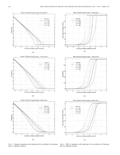
292 IEEE TRANSACTIONS ON CIRCUITS AND SYSTEMS FOR VIDEO TECHNOLOGY, VOL. 7, NO. 2, APRIL 1997 (a) (a) (b) (b) (c) Fig. 5. Entropy of quantizers with dead-zone <strong>for</strong> (a) uni<strong>for</strong>m, (b) Gaussian, <strong>and</strong> (c) Laplacian sources. (c) Fig. 6. MSE of quantizers with dead-zone <strong>for</strong> (a) uni<strong>for</strong>m, (b) Gaussian, <strong>and</strong> (c) Laplacian sources.
HANG AND CHEN: SOURCE MODEL FOR TRANSFORM VIDEO CODER AND ITS APPLICATION—PART I 293 Reference curves shown on those plots are the asymptotic <strong>for</strong>mulas described by (9) <strong>and</strong> (10). In image coding, the quantization step sizes of significant frequency components are usually smaller than the signal st<strong>and</strong>ard deviation; there<strong>for</strong>e, (10) <strong>and</strong> (12) are reasonably good approximations if , , <strong>and</strong> are adjusted appropriately. The values of these parameters, in general, depend upon <strong>and</strong> . However, <strong>for</strong> a fixed <strong>and</strong> a certain range of step sizes, they can be approximated by constants. When the step size gets larger, (10) <strong>and</strong> (12) become less accurate. But in these cases the b<strong>its</strong> produced by those coefficients are very small <strong>and</strong> thus do not change very much the total b<strong>its</strong>. Extensions <strong>and</strong> modifications of these parameters are described in the next section. Assuming that the b<strong>its</strong> on the average needed to encode an above-threshold trans<strong>for</strong>m coefficient are represented by [from (12)] (21) these curves <strong>and</strong> have about the same value <strong>for</strong> all the three distributions. There<strong>for</strong>e, replacing in (23) by ,we obtain where (25) where , is the threshold value used in picking up the th trans<strong>for</strong>m coefficient, <strong>and</strong> <strong>and</strong> are sourcedependent parameters. The average b<strong>its</strong> number of a pixel becomes Or (26) (27) (22) where are the b<strong>its</strong> <strong>for</strong> the end-of-block signal. If the weighting matrix in (17) is adopted, the average b<strong>its</strong> <strong>and</strong> the average distortion can be made more explicit <strong>and</strong> (23) (24) Since the threshold trans<strong>for</strong>m coding with weighting matrix is invented to match the subjective distortion criterion, the mean square error distortion calculation, (24), is not as useful as the b<strong>its</strong> calculation, (23), which can be used to adjust the quantization step <strong>for</strong> regulating encoder buffer <strong>and</strong> controlling picture quality. If is chosen to be with roughly the same constant value <strong>for</strong> all the coefficients, then , , <strong>and</strong> can be expressed as functions of <strong>and</strong> only. Also, in most image coding cases, the ac components have approximately Laplacian distribution <strong>and</strong> the dc component, uni<strong>for</strong>m or Gaussian distribution [12]. Hence, the values are similar <strong>for</strong> all the frequency components as indicated by Fig. 5, in which ’s are proportional to the slopes of with . Note that we denote by in the above equations <strong>for</strong> simplicity. The direct use of (25) seems to be fairly complicated—it needs to estimate a number of parameters, ’s, ’s, <strong>and</strong> , computed from image data. If, however, we could assume that the picture to be coded is not much different from the picture that has already been coded in the sense that the , <strong>and</strong> remain about the same in the neighborhood of that we are dealing with, then the parameter in (27) can be estimated from the <strong>and</strong> of the coded pictures. Typically, the value is less picture-dependent, only the value has to be estimated from image data. Consequently, the entire model identification procedure can be relatively simple. V. MODEL PARAMETERS For a practical application, the parameters of the above model have to be adjusted to cope with the specific video coder used <strong>and</strong> the real picture characteristics. The meaning of the parameters in our model (23) <strong>and</strong> (24) suggests the following modifications. First, since is a factor mainly determined by probability distribution, we assume is a constant ( 1.2 <strong>for</strong> Laplacian source, say) <strong>for</strong> the rest of analysis. Second, the value of is no longer constant <strong>for</strong> small ; however, those values can be precalculated <strong>and</strong> stored in a table <strong>for</strong> real-time applications. Third, the constant is replaced by a parametric function to compensate <strong>for</strong> the mismatch between the ideal model <strong>and</strong> a practical video coder. Although these parameters ( , , <strong>and</strong> ) may be somewhat related, <strong>for</strong> simplicity we study them separately. We will elaborate on the second <strong>and</strong> the third items below.