A Probabilistic Approach to Geometric Hashing using Line Features

A Probabilistic Approach to
Geometric Hashing using Line Features
by
Frank Chee-Da Tsai
a dissertation submitted in partial fulfillment
of the requirements for the degree of
Doctor of Philosophy
Department of Computer Science
New York University
September 1993
Approved:
Professor Jacob T. Schwartz
Research Advisor

cæ Frank Chee-Da Tsai
All Rights Reserved, 1993.

Dedication
This dissertation is dedicated to Professor Jacob T. Schwartz for his invaulable advisory,
to my parents for their endless love and to Buddha, whose wisdom cheers me through the
dark patches of my life.
iii

Acknowledgements
My most sincere gratitude goes to my research advisor Professor Jacob T. Schwartz
for his generous guidance, without which this dissertation can not be possible. To whom,
I also owe the understanding of identifying research directions of scientiæc interest.
Iwould also like to express my gratitude to Professor Wen-Hsiang Tsai of National
Chiao-Tung University, Hsin-Chu, Taiwan, Republic of China. I took his course ëImage
Processing" when I was an undergraduate senior. This is my ærst taste of applying computer
technology to the processing of images. After two-year R.O.T.C. military service
upon graduation, I came here to the Courant Institute in 1987 to further my study. Professor
Stçephane Mallat's ëComputer Vision" course again intrigued my interest in the æeld
of image analysis.
Thanks are also due to Professor Jaiwei Hong, Professor Robert Hummel, Professor
Richard Wallace, Professor Haim Wolfson, Dr. Isidore Rigoutsos, Mr. Ronie Hecker and
Mr. Jyh-Jong Liu for various kinds of helps and discussions.
I also thank the staæs in the Courant Robotics Laboratory, for the days we worked
together, especially Dr. Xiaonan Tan for her encouragement.
Finally, I thank my parents, truly and sincerely, for their patience, support and constant
encouragement throughout the work and my whole life.
iv

Abstract
One of the most important goals of computer vision research is object recognition.
Most current object recognition algorithms assume reliable image segmentation, which in
practice is often not available. This research exploits the combination of the Hough method
with the geometric hashing technique for model-based object recognition in seriously degraded
intensity images.
We describe the analysis, design and implementation of a recognition system that can
recognize, in a seriously degraded intensity image, multiple objects modeled by a collection
of lines.
We ærst examine the factors aæecting line extraction by the Hough transform and proposed
various techniques to cope with them. Line features are then used as primitive
features from which we compute the geometric invariants used by the geometric hashing
technique. Various geometric transformations, including rigid, similarity, aæne and
projective transformations, are examined.
We then derive the ëspread" of computed invariant over the hash space caused by
ëperturbation" of the lines giving rise to this invariant. This is the ærst of its kind for
noise analysis on line features for geometric hashing. The result of the noise analysis is
then used in a weighted voting scheme for the geometric hashing technique.
We have implemented the system described and carried out a series of experiments on
polygonal objects modeled by lines, assuming aæne approximations to perspective viewing
transformations. Our experimental results show that the technique described is noise
resistant and suitable in an environment containing many occlusions.
v

Contents
List of Figures
ix
1 Introduction 1
1.1 Model-Based Object Recognition : : : : : : : : : : : : : : : : : : : : : : : : 2
1.1.1 Problem Deænition : : : : : : : : : : : : : : : : : : : : : : : : : : : : 2
1.1.2 Object Recognition Method : : : : : : : : : : : : : : : : : : : : : : : 3
1.2 Diæculties to Be Faced : : : : : : : : : : : : : : : : : : : : : : : : : : : : : 5
1.3 The Hashing Approach : : : : : : : : : : : : : : : : : : : : : : : : : : : : : : 5
1.4 Overview of This Dissertation : : : : : : : : : : : : : : : : : : : : : : : : : : 6
1.4.1 Line Extraction : : : : : : : : : : : : : : : : : : : : : : : : : : : : : : 7
1.4.2 Line Invariants : : : : : : : : : : : : : : : : : : : : : : : : : : : : : : 7
1.4.3 Eæect of Noise on Line Invariants : : : : : : : : : : : : : : : : : : : : 7
1.4.4 Invariant Matching with Weighted Voting : : : : : : : : : : : : : : : 7
2 Prior and Related Work 9
2.1 Basic Paradigms : : : : : : : : : : : : : : : : : : : : : : : : : : : : : : : : : 9
2.1.1 Template Matching : : : : : : : : : : : : : : : : : : : : : : : : : : : : 9
2.1.2 Hypothesis-Prediction-Veriæcation : : : : : : : : : : : : : : : : : : : 10
2.1.3 Transformation Accumulation : : : : : : : : : : : : : : : : : : : : : : 11
2.1.4 Consistency Checking and Constraint Propagation : : : : : : : : : : 13
2.1.5 Sub-Graph Matching : : : : : : : : : : : : : : : : : : : : : : : : : : : 14
2.1.6 Evidential Reasoning : : : : : : : : : : : : : : : : : : : : : : : : : : : 15
2.1.7 Miscellaneous : : : : : : : : : : : : : : : : : : : : : : : : : : : : : : : 15
2.2 An Overview of Geometric Hashing : : : : : : : : : : : : : : : : : : : : : : : 17
vi

2.2.1 A Brief Description : : : : : : : : : : : : : : : : : : : : : : : : : : : : 17
2.2.2 Strengths and Weaknesses : : : : : : : : : : : : : : : : : : : : : : : : 19
2.2.3 Geometric Hashing Systems : : : : : : : : : : : : : : : : : : : : : : : 20
2.3 The Bayesian Model of Rigoutsos : : : : : : : : : : : : : : : : : : : : : : : : 20
3 Noise in the Hough Transform 23
3.1 The Hough Transform : : : : : : : : : : : : : : : : : : : : : : : : : : : : : : 23
3.2 Various Hough Transform Improvements : : : : : : : : : : : : : : : : : : : : 25
3.3 Implementation and Measured Performance : : : : : : : : : : : : : : : : : : 27
3.4 Some Additional Observations Concerning the Accuracy of Hough Data : : 36
4 Invariant Matching Using Line Features 39
4.1 Change of Coordinates in Various Spaces : : : : : : : : : : : : : : : : : : : 39
4.1.1 Change of Coordinates in Image Space : : : : : : : : : : : : : : : : : 40
4.1.2 Change of Coordinates in Line Parameter Space : : : : : : : : : : : 40
4.1.3 Change of Coordinates in èç; rè Space : : : : : : : : : : : : : : : : : 41
4.2 Encoding Lines by a Basis of Lines : : : : : : : : : : : : : : : : : : : : : : : 42
4.3 Line Invariants under Various Transformation Groups : : : : : : : : : : : : 43
4.3.1 Rigid Line Invariants : : : : : : : : : : : : : : : : : : : : : : : : : : : 43
4.3.2 Similarity Line Invariants : : : : : : : : : : : : : : : : : : : : : : : : 46
4.3.3 Aæne Line Invariants : : : : : : : : : : : : : : : : : : : : : : : : : : 51
4.3.4 Projective Line Invariants : : : : : : : : : : : : : : : : : : : : : : : : 55
5 The Eæect of Noise on the Invariants 60
5.1 A Noise Model for Line Parameters : : : : : : : : : : : : : : : : : : : : : : : 60
5.2 The Spread Function of the Invariants : : : : : : : : : : : : : : : : : : : : : 61
5.3 Spread Functions under Various Transformation Groups : : : : : : : : : : : 64
5.3.1 Rigid-Invariant Spread Function : : : : : : : : : : : : : : : : : : : : 64
5.3.2 Similarity-Invariant Spread Function : : : : : : : : : : : : : : : : : : 65
5.3.3 Aæne-Invariant Spread Function : : : : : : : : : : : : : : : : : : : : 67
5.3.4 Projective-Invariant Spread Function : : : : : : : : : : : : : : : : : : 69
vii

6 Bayesian Line Invariant Matching 74
6.1 A Measure of Matching between Scene and Model Invariants : : : : : : : : 74
6.2 Evidence Synthesis by Bayesian Reasoning : : : : : : : : : : : : : : : : : : : 76
6.3 The Algorithm : : : : : : : : : : : : : : : : : : : : : : : : : : : : : : : : : : 77
6.4 An Analysis of the Number of Probings Needed : : : : : : : : : : : : : : : : 78
7 The Experiments 80
7.1 Implementation of Aæne Invariant Matching : : : : : : : : : : : : : : : : : 80
7.2 Best Least-Squares Match : : : : : : : : : : : : : : : : : : : : : : : : : : : : 82
7.3 Experimental Results and Observations : : : : : : : : : : : : : : : : : : : : 85
8 Conclusions 95
8.1 Discussion and Summary : : : : : : : : : : : : : : : : : : : : : : : : : : : : 95
8.2 Future Directions : : : : : : : : : : : : : : : : : : : : : : : : : : : : : : : : : 96
A 98
B 100
Bibliography 102
viii

List of Figures
3.1 A comparison of the results of the standard Hough technique and our improved
Hough technique, when applied to an image without noise. : : : : : 28
3.2 A comparison of the results of the standard Hough technique and our improved
Hough technique, when applied to a noisy image. : : : : : : : : : : : 29
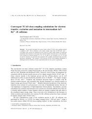
3.3 The twenty models used in our experiments. From left to right, top to
bottom are model-0 to model-19. : : : : : : : : : : : : : : : : : : : : : : : : 30
3.4 Reading from top to bottom, left to right, è0è to è8è are image-0 with different
noise levels corresponding to cases 0 to 8. : : : : : : : : : : : : : : : 32
3.5 Image-1 to Image-9 before noise is imposed. The same noise levels as for
Image-0 are applied during our experiments. : : : : : : : : : : : : : : : : : 33
3.6 The thicker line is with parameter èç; rè. Projections of the pixels of this
line onto line èç +90 æ ;rè will disperse around the position r distant from
the origin. : : : : : : : : : : : : : : : : : : : : : : : : : : : : : : : : : : : : : 38
7.1 Experimental Example 1 : : : : : : : : : : : : : : : : : : : : : : : : : : : : : 87
7.2 Experimental Example 2 : : : : : : : : : : : : : : : : : : : : : : : : : : : : : 88
7.3 Experimental Example 3 : : : : : : : : : : : : : : : : : : : : : : : : : : : : : 89
7.4 Experimental Example 4 : : : : : : : : : : : : : : : : : : : : : : : : : : : : : 90
7.5 Experimental Example 5 : : : : : : : : : : : : : : : : : : : : : : : : : : : : : 92
7.6 Experimental Example 6 : : : : : : : : : : : : : : : : : : : : : : : : : : : : : 93
ix

Chapter 1
Introduction
One of the most important goals of computer vision research is object recognition. This
humanlike visual capability would enable machines to sense and analyze their environment
and to take an appropriate action as desirable.
We consider intensity-image techniques. Range data is usually harder to obtain. There
is also reason to believe that human vision emphasizes intensity images and that most
practical applications of computer vision can be tackled without range information ë42ë.
Speciæcally, we consider the problem of 2-D èor, æat 3-Dè object recognition under various
viewing transformations. We are interested in è1è large model bases èmore than ten
objectsè; è2è cluttered scene èlow signal noise ratioè; è3è high occlusion levels; è4è segmentation
diæculties. The current approaches to image segmentation generally produce
incomplete boundaries and extraneous edge indications. Therefore, any approach to object
recognition has to cope with segmentation defects. To work in environments containing
many occlusions, we impose minimal segmentation requirements | only positional information
of edgels is assumed to be available.
We will describe the analysis, design and implementation of a recognition system that
can recognize, in a seriously degraded intensity image, multiple objects which can be
modeled as collections of lines.
1

CHAPTER 1. INTRODUCTION 2
1.1 Model-Based Object Recognition
Recognition can be achieved by establishing correspondences between many kinds of predicted
and measured object properties, including shape, color, texture, connectivity, context,
motion, or shading. Here, we will focus upon the problem of achieving spatial correspondence.
This is often prerequisite to examining correspondences along the other
dimensions.
Prior research ë7,13ë has indicated that a model-based approach to object recognition
can be very eæective inovercoming occlusion, complication and inadequate or erroneous
low level processing. Most commercial vision systems are model-based ones, in which
recognition involves matching an input image to a set of predeæned models of objects. A
key goal in this approach is to precompile a description of a known set of objects, then to
use these object models to recognize in an image each instance of an object and to specify
its position and orientation relative to the viewer.
1.1.1 Problem Deænition
Object recognition can be conceptualized in various ways. A brief survey of the literature
on this subject demonstrates this point ë7,8,13ë. Here, we adopt the deænition given by
Besl and Jain ë7ë.
Their deænition is motivated by the observation of human visual capabilities. Two
main steps are involved. The ærst step is learning. When a new object is given, human
visual system gathers information about that object from many diæerent viewpoints. This
process is usually referred to as model formation. The second step is identiæcation.
The following deænition of the single-arbitrary-view model-based object recognition problem
is motivated by the above:
1. Given any collection of labeled solid objects, èaè each object can be examined as long
as the object is not deformed; èbè labeled models can be created using information
from this examination.
2. Given digitized sensor data corresponding to one particular, but arbitrary æeld of
view of the real world, given any data stored previously during the model formation
process, and given the list of distinguishable objects, the following questions must be
answered:

CHAPTER 1. INTRODUCTION 3
æ Does the object appear in the digitized sensor data ?
æ If so, how many times does it occur ?
æ For each occurrence, è1è determine the location in the sensor data èimageè, è2è
determine the location èor translation parametersè of that object with respect
to a known coordinate system èif possible with given sensorè, and è3è determine
the orientation èor rotation parametersè with respect to a known coordinate
system.
This problem statement allows the possibility of using computers to solve it; at any
rate the problem is clearly solvable by human beings.
1.1.2 Object Recognition Method
In most object-recognition systems, one can distinguish æve sub-processes: image formation,
feature extraction, model representation, scene analysis and hypotheses veriæcation.
Image Formation
This process creates images via sensors, which can be sensitive toavariety of signals like
visible spectrum light, X-rays, etc. As said, we will concentrate on intensity images.
Feature Extraction
This process acts on the sensor data and extracts relevant features. The geometric features
we are interested in might in principle be lines, segments, curvature extrema, curvature
discontinuities, conics and so on. But we will use lines exclusively.
Model Representation
This process converts models to the quantities which will be used to recognize them. This
process is closely related to the feature-extracting process, since the same features are
supposed to be extracted from a scene for matching.
Models based on geometric properties of an object's visible surfaces or silhouette are
commonly used because they describe objects in terms of their constituent shape features.
Although many other models of regions and images emphasizing gray-level properties èe.g.

CHAPTER 1. INTRODUCTION 4
texture and colorè have been proposed, solving the problem of spatial correspondence is
often a prerequisite to their use. Thus, recognition of objects in a scene is always apt to
involve construction of a shape description of objects from sensed data and then matching
the description to stored object models.
A shape representation scheme usually involves at least two components:
1. the primitive units, e.g. vertices è0-dimensionè, curves and edges è1-dimensionè, surfaces
è2-dimension, e.g. plane surface, quadratic surfaceè and volumes è3-dimension,
e.g. generalized cylindersè;
2. the way those primitives are combined to form the object models.
Such a representation scheme must satisfy the following two criteria to be considered of
good quality:
1. Near-Uniqueness: Ideally each object in the world should have a limited number of
representations; otherwise, when image features are derived, there will be also many
choices of conæguration for each representation and thus increase the computational
complexity to match conægurations of image features to model representations.
2. Continuity: Similar objects should have similar representations and very diæerent
objects should have very diæerent representations.
Scene Analysis
This process involves an algorithm for performing matching between models and scene
descriptions. This process is most crucial in an object recognition system and is the focus
of this thesis. It recovers the transformations the model objects undergo during the imageformation
process. Sometimes a quality measure can be associated with each model instance
detected; this measure can be used as a measure of belief for further decision making in
an autonomous system. We will classify basic matching techniques and review them in
chapter 2. The techniques we are interested in involve those allowing partial occlusion,
viewing distortion and data perturbation.
In this dissertation, we will focus on using the geometric hashing technique for matching.
The geometric hashing technique is very good as a ælter capable of eliminating many
candidate hypotheses as the identity of the objects ë38ë.

CHAPTER 1. INTRODUCTION 5
Hypotheses Veriæcation
This process evaluates the quality of surviving hypotheses and either accepts or rejects
them. Usually an object recognition system projects the hypothesized models onto the
scene and the fraction of the model accounted for by the available scene signals is computed.
If this fraction is below a pre-set èusually obtained empiricallyè threshold, the hypothesis
fails veriæcation.
1.2 Diæculties to Be Faced
What makes the visual recognition task diæcult ? Basically, there are four factors:
1. noise, e.g. sensor noise and bad lighting conditions;
2. clutter, e.g. industrial parts occluded by æakes generated in the milling process;
3. occlusion, e.g. industrial parts overlapping each other;
4. spurious data, e.g. presence of unfamiliar objects in the scene.
The amount of eæort required to recognize and locate the objects increases when these
four factors become serious. In dealing with these four factors, we have to consider three
problems ë13ë:
1. What kind of ëfeatures" should and can be reliably be extracted from an image in
order to adequately describe the spatial relations in a scene ?
2. What constitutes an eæective representation of these features and their relationships
for an object model ?
3. How should the correspondence between scene features and model features be matched
in order to recover model instances in a complex scene ?
1.3 The Hashing Approach
In order to recognize 3-D objects in 2-D images, we must either perform a comparison
in 2-D or 3-D. Since it is easier to project 3-D models onto a 2-D image than it is to

CHAPTER 1. INTRODUCTION 6
reconstruct 3-D shapes from 2-D scenes, it is logical, in model-based vision, to perform the
comparisons in image space. If we simply project the 3-D models onto image space during
the recognition process, we must guess at the projection parameters, and incur the computational
expense of multiple projections at run-time. If we precompute many projections,
then we potentially substitute many 2-D models for relatively fewer 3-D models.
A more eæective method of performing object recognition was proposed by Schwartz
and Sharir ë33ë. The technique exploits the idea of hashing. By appropriately selecting a
hash function, dictionary operations 1 can be performed in Oè1è time on the average. By
hashing transformation invariants, instead of raw data subject to a viewing transformation,
the hash function ëhashes" to a æxed ëbucket" of the hash table before and after whatever
viewing transformations are allowed. Thus object models can be represented by its
constituent geometric features, some appropriate subset of which is hashed and pre-stored
in the hash table in a redundant way. During recognition, the same hash operations are
applied to a subset of scene features and candidate matching model features are retrieved
from the hash table to hypothesize their correspondence.
This hashing technique trades space for time. We mayeven pre-compute many projections,
substituting many 2-D models for relatively fewer 3-D models.
1.4 Overview of This Dissertation
In this dissertation, we consider highly degraded intensity images containing multiple objects.
We emphasize use of four techniques:
æ Use of an improved Hough transform to detect line features in a noisy image;
æ Use of geometric invariants derived from line features under various viewing transformations;
æ Use of the eæect of line feature statistics on the perturbation analysis of invariants
computed;
æ Use of a Bayesian reasoning as the basis for line feature matching.
1 consisting of ëinsert", ëdelete" and ëmember" operations ë1ë.

CHAPTER 1. INTRODUCTION 7
1.4.1 Line Extraction
In noisy scenes, the locations of point features can be hard to detect. Line features are
more robust and can be extracted by the Hough transform method with greater accuracy.
Thus we choose lines as the primitive features to be used.
In chapter 3, we ærst brieæy review the Hough transform technique for detecting line
features. Then we point out several factors that adversely aæect the performance of the
method and propose several heuristics to cope with those factors to improve the performance.
A series of experiments relating to this point are presented.
1.4.2 Line Invariants
In chapter 4, we ærst examine the way in which coordinate changes act on various spaces
of potential interest for recognition. This allows us to deæne a method of encoding a line
using a combination of other lines in a way invariant under suitable geometric transformations.
Potentially interesting transformations considered include rigid, similarity, aæne
and projective transformations.
1.4.3 Eæect of Noise on Line Invariants
In chapter 5, we model the statistical behavior of line parameters detected by the Hough
transform in a noisy image using a Gaussian random process with mild assumptions. We
analyze the statistics of the computed invariants and show that these have a Gaussian
distribution in a ærst order approximation.
Analytical formulae for various transformations including rigid, similarity, aæne and
projective transformations are given.
1.4.4 Invariant Matching with Weighted Voting
In chapter 6, we use the result of chapter 5 to formulate a Bayesian maximum likelihood
pattern classiæcation as the basis of weighted voting scheme for matching line features by
Geometric Hashing.
We have implemented a system that makes use of these ideas to perform object recognition,
assuming aæne approximations to more general perspective viewing transformations.

CHAPTER 1. INTRODUCTION 8
Both synthesized and real images were used in experiments. Experimental results are given
in chapter 7. It is seen that the technique is noise resistant and usable in environments
containing many occlusions.

Chapter 2
Prior and Related Work
Numerous techniques have been proposed for object recognition. A brief survey and classiæcation
of those techniques is given below. These techniques are not independent of each
other; most vision systems combine several of them.
We divide the analysis into three sections. The ærst section examines object recognition
using various classical schemes, and the second two sections discuss the background and
existing work in the æeld of geometric hashing. In this thesis, we study the Hough transform
methods, discussed in section 2.1.3 and geometric hashing described in section 2.2. Our
work directly builds upon the Bayesian weighted voting scheme of Rigoutsos, which we
describe in section 2.3.
2.1 Basic Paradigms
2.1.1 Template Matching
Template matching involves matching an image to a stored representation and evaluating
some æt function.
According to their æexibility, templates can be classiæed into four categories ë14ë:
æ Total templates require an exact match between a scene and a template. Any displacement
or orientation error of pattern in the scene will result in rejection.
æ Partial templates move a template across the scene, computing cross-correlation factors.
Points of maximum cross-correlation values are considered as locations where
9

CHAPTER 2. PRIOR AND RELATED WORK 10
the desired pattern appears; multiple matches against the scene is thus possible.
æ Piece templates represent a pattern by its components. Usually the component templates
are weighted by size and scored against a prototype list of expected features.
This method is less sensitive to distortions of the pattern in the scene than the more
limited techniques listed above. The subgraph matching technique described later
can be viewed as an extension to this technique.
æ Flexible templates are designed to handle the problems of scene deviations from prototypes.
Starting with a good prototype of a known object, templates can be parametrically
modiæed to obtain a better æt until no more improvement is obtained.
èThis technique has been successfully applied to the sorting of chromosome images.è
A diæculty is that æexible approaches tend to be more time-expensive than rigid
approaches.
Most of these template matching techniques apply only in two-dimensional cases and have
little place in three-dimensional analysis, where perspective distortion comes into play.
One can store a dense set of tessellations of possible views, but this results in enormous
computational time in matching. For basic techniques of template matching, see ë15ë.
2.1.2 Hypothesis-Prediction-Veriæcation
The hypothesis-prediction-veriæcation approach is among the most commonly-used techniques
in vision systems. It combines both bottom-up and top-down paradigms.
Hypotheses are generated bottom-up among structures in a geometric hierarchy, from
structures of edges to curves, from structures of curves to surfaces, and from structures
of surfaces to objects. Predictions work top-down from object models to images. Once
ahypothesis has been made, predictions and measurements provide new information for
identiæcation.
Many such schemes use geometric features such as arcs, lines and corners to construct
model representations. These features are usually portions of the object's boundary.
In the HYPER system ë4ë, both model and scene are represented in the same way
by approximating the boundary with polygons. The ten longest segments are chosen as
so-called privileged segments which are the focus features used to detect a prospective

CHAPTER 2. PRIOR AND RELATED WORK 11
correspondence èhypothesisè between object models and the scene. Using this correspondence,
a transformation can be computed and nearby features are sought èpredictionè. The
privileged segments, together with their nearby features, are combined to compute a new
transformation. Then the veriæcation step follows.
Veriæcation is often accomplished using an alignment method. Usually there is a tradeoæ
between the hypothesis generation stage and the veriæcation stage. If hypotheses are
generated in a quick-and-dirty manner, then the veriæcation stage requires more eæort. If
we want the veriæcation stage to be less pains-taking, then more reliable features have to
be detected and more accurate hypotheses produced.
In alignment by Huttenlocher and Ullman ë30,31ë, they consider aæne approximations
to more general perspective transformations, using alignments of triplets of points. Models
are processed sequentially during recognition. For each model, an exhaustive enumeration
of all the possible pairings of three non-collinear points of the model and the scene is
exercised. Thus the alignment method heavily relies on veriæcation. As a transformation
is determined by the correspondence of model and scene features, the model is transformed
and aligned to superimpose the image. Veriæcation of the entire edge contour, rather than
just a few local feature points, is then performed to reduce the false alarm rate. To cope
with the high computational cost of the veriæcation stage, a hierarchical scheme is used:
Starting with a relatively simple and rapid check, they eliminate many false matches, and
then conclude with a more accurate and slower check.
To sum up, the hypothesis-prediction-veriæcation cycle relates scene images to object
models and object models to scene images step by step with reænement in each step.
Note also that any scheme using the ëhypothesis-prediction-veriæcation" paradigm can
be tailored to a parallel implementation by using the overwhelming computing power to
generate a great number of hypotheses concurrently and do veriæcations concurrently.
2.1.3 Transformation Accumulation
Transformation accumulation is also called pose clustering ë50ë or the generalized Hough
transform ë5ë, which ischaracterized by a ëparallel" accumulation of low level pose evidences,
followed by a clustering step which selects pose hypotheses with strong support
from the set of evidences.
This method can be viewed as the inverse of template matching, which moves the model

CHAPTER 2. PRIOR AND RELATED WORK 12
template around all the positions of the scene and directly computes a value èusually crosscorrelationè
as a measure of matching. Transformation accumulation, instead of trying all
possible positions of the model in the scene, computes which positions are consistent with
model features and scene features. Moreover, its use of all of the evidences without regard
to their order of arrival can be advantageous when there are occlusions.
The features used to generate pose hypotheses can be of high level or low level. If the
level of features used are high enough, much less computational eæort is required for the
accumulation stage. However, the trade-oæ is that higher level features are usually more
diæcult to extract.
The major problem of this technique usually lies in ensuring that all visible hypotheses
are considered within acceptable limits of storage and computational resources. However,
as computer power continues to grow while its cost continues to drop, this problem has
been growing steadily less signiæcant.
In the generalized Hough transform ë5ë, the transformation between a model and the
scene is usually described by a set of transformation parameters. For example, four parameters
are needed for the case of two-dimensional similarity transformations: two parameters
for translation; one parameter for rotation; one parameter for scaling. Each transformation
parameter is quantized in the so-called Hough space. The scene features vote for
these parameters which are consistent with the pairings of these scene features and hypothesized
model features. One problem of the generalized Hough transform is the size
of the Hough space. In terms of two-dimensional cases, we face three-dimensional Hough
space for rigid transformations; four-dimensional Hough space for similarity transformations;
six-dimensional Hough space for aæne transformations.
Tucker et al. ë53ë use local boundary features to constrain an object's position and
orientation, which is then used as the basis for hypothesis generation. Their system takes
advantage of the highly parallel processing power of the Connection Machine ë26ë to generate
numerous transformation hypotheses concurrently and verify them concurrently. The
number of processors required for each model is equal to the number of features of the
model. Each scene feature participates, in parallel, independently in each processor to
match model features for generating transformation hypotheses, which, after veriæed, are
used for evidence accumulation for voting for the pose transformation of the object.

CHAPTER 2. PRIOR AND RELATED WORK 13
Thompson and Mundy ë52ë describe a system for locating objects in a relatively unconstrained
environment. The availability of a three-dimensional surface model of a polyhedral
object is assumed. The primitive feature used is the so-called vertex-pair, which consists
of two vertices: one is characterized by its position coordinate; the other, in addition to
position coordinate, includes two edges that deæne the vertex. This feature serves as the
basis of computing the aæne viewing transformation from the model to the scene. Through
the voting in the transformation space, candidate transformations are selected.
A common critique about this paradigm lies in that as the scene is noisy, the accumulation
of ëevidences" contributed by random noises can possibly result in false alarms.
Grimson and Huttenlocher ë22ë give a formal analysis of the likelihood of false positive
responses of the generalized Hough transform for object recognition. However, we can use
this paradigm as an early stage of processing èi.e., as a ælterè, followed by a scrutinized
veriæcation stage.
2.1.4 Consistency Checking and Constraint Propagation
Many model-based vision schemes are based on searching the set of possible interpretations,
which is usually combinatorially large.
As in other areas of artiæcial intelligence, making use of large amounts of world knowledge
can often lead not only to increased robustness but also to a reduction in the search
pace that must be explored during the process of interpretation. It is usually possible to
analyze a number of constraints or consistency conditions that must be satisæed to make
a correct interpretation. Eæective application of consistency checking or propagation of
constraints during searching can often prune the search space greatly.
Lowe ë41ë emphasizes the importance of viewpoint consistency constraint, which requires
that the locations of all object features in an image be consistent with the projection
from a single viewpoint. The application of this constraint allows the spatial information
in an image to be compared with prior knowledge of an object's shape to the full degree
of available image resolution. Lowe also argues that viewpoint-consistency plays a central
role in most instances of human visual recognition.
Grimson ë20ë extended his previous work RAF ë23ë to handle some classes of parameterized
objects. He approaches the recognition problem as a searching problem using the

CHAPTER 2. PRIOR AND RELATED WORK 14
so-called interpretation tree. Since this search is inherently an exponential process, he analyzed
a set of geometric constraints based on the local shape of parts of objects to prune
large subtrees from consideration without having to explore them.
The relaxation labeling technique èe.g. ë51,54ëè is yet another example of this type.
Many visual recognition problems can be viewed as constraint-satisfaction problems. For
example, when labeling a block-world picture, a relaxation algorithm iteratively assigns
values to mutually constrained objects using local information alone in such away that
ensures a consistent set of values for which no constraints are violated. The values assigned
to the objects by relaxation algorithms can be discrete or probabilistic. In the former case,
discrete levels are assigned to objects, while in the latter case, a level of certainty èor
probabilityè is attached to each label. Relaxation algorithms can proceed in a paralleliterative
manner, propagating matching constraints in parallel.
2.1.5 Sub-Graph Matching
Both object models and scene images can be expressed by graphs of nodes and arcs. Nodes
represent features èusually geometric structuresè detected and arcs represent the geometric
relations between these features, e.g. ë11ë. The task then reduces to ænd an embedding or
ætting of a model in a description of the scene.
Since a model contains both local and relational features in the form of a graph, matching
depends not only on the presence of particular boundary features but also on their
interrelations èe.g. distanceè. The requirement for successful recognition is that a suæcient
set of key local features have to be visible and in correct relative positions, which may
allow for a speciæed amount of distortion. For example, Bolles and Cain ë10ë proposed the
use of a hierarchy of local focus features for model representation. Once the local focus
features have been detected, nearby features are predicted and searched for in the scene.
If the best focus features are occluded, the second best focus features are used.
An advantage of this technique is its robustness to relative occlusion and distortion.
Computational ineæciency can be a drawback, since graph-matching or subgraph isomorphism
procedures have to be executed. Eæective strategies to reduce the time complexity
are therefore required. In ë10ë, once an occurrence of the best focus feature is located, the
system simply runs down the appropriate list of nearby features and a transformation is
computed, followed by averiæcation step. Thus exploration of the whole relational graph

CHAPTER 2. PRIOR AND RELATED WORK 15
is avoided. Barrow and Tenenbaum ë6ë proposes use of a hierarchical graph-searching
technique which decomposes the model into independent components.
2.1.6 Evidential Reasoning
Evidential reasoning is a method for combining information from diæerent sources of evidence
to update probabilistic expectations. The attractive feature of using evidential
reasoning for computer vision is that it allows us to combine information of varying reliability
from many sources, even though no particular item of evidence is by itself strong
enough for recognizing a particular object.
For example, SCERPO by Lowe ë40ë is a search-based matching system. As to the
search space of SCERPO, two major components are involved: è1è the space of possible
viewpoints; è2è the space of selecting one model from the model database. Lowe tackles
the ærst component by perceptual organization and suggests that the second component
be treated by a technique of evidential reasoning. Each piece of evidence contributes
to the presence of a certain object or objects, which quantitatively can be described by a
probabilistic expectation. The combining of evidences thus can be quantitatively described
by combining probabilistic expectations. The probability ranking is constantly updated to
reæect new evidence found. For example, as soon as one object is recognized, it provides
contextual information which updates the rankings and aids in the search process. Ranking
and updating may take time; however, as the list of possible objects increases, cost of the
evidential reasoning may be amortized and its use becomes more important.
To sum up, evidential reasoning may deserve serious consideration to be incorporated
into a system under development. It shows promise for carrying out the objective of
combining many sources of information, including color, texture, shape and prior knowledge
in a æexible way toachieve recognition.
2.1.7 Miscellaneous
Dual Models
If partial visibility problem is to be attacked, a recognition system using global features
alone can not be feasible. Only local features can be used in the matching procedure in
order to cope with overlapping parts and occlusions. One is free to choose diæerent local

CHAPTER 2. PRIOR AND RELATED WORK 16
features such aspoints, lines, curves, etc., or their combinations as the matching features,
according to the nature of the objects in the model base. However, two factors of representation,
completeness and eæciency, have to be taken into consideration. Completeness
of representation suggests rich enough features in order to enable discrimination between
similar objects; while eæciency suggests using some minimal characteristic information to
match models again the scene èso that the inherent complexity of the matching algorithm
will be smallè.
A main drawback of representation by local features can be its incompleteness, since
objects usually can not be fully described by a set of local features alone. One way to cope
with this problem is to use both global and local feature representations: Local features
are used in the matching procedure; while the additional complete representation is used,
after the matching process, for veriæcation and further reænement of the object localization
ë4,10,19,31,36ë.
Dual Scenes
Object recognition algorithms usually fall into two categories í those using intensity images
and those using range data. However, we may use both of them as long as it helps.
For example, Kishon ë34ë combines the use of both range and intensity data to extract
3-D curves from a scene. These curves will be of a much higher quality than if they were
extracted from the range data alone. The combined information is also used to classify the
3-D curves as either shadow, occluding, fold or painted curves.
Abstracted Features
An abstracted feature is a feature which does not physically exist, but is inferred. For
example, in preparing a model representation for polygonal objects, we may extend nonneighboring
edges to obtain their intersection and use the contained angle as a feature.
Some more advanced applications of using abstracted features include the footprint of
concavity ë37ë, the Fourier Descriptor used for silhouettes description of aircraft in ë2ë and
the representation of turning angle as a function of arc length used in ë3,19,49ë.

CHAPTER 2. PRIOR AND RELATED WORK 17
Normalization
There are various reasons for the use of normalization.
In some cases, it is used to preserve certain properties. For example, in the probabilistic
relaxation labeling scheme, the accumulated contributions from neighboring points have to
be normalized so that the updating rule results in a probability èi.e., a value in ë0::1ëè.
In other cases, it can be viewed as a technique for removing some uncertain factors. For
example, suppose we use Fourier Descriptor to describe the boundary of an object. In order
for such representation insensitive to the variations as changes in size, rotation, translation
and so on, we have to perform the normalization operations such that the contour has a
ëstandard" size, orientation and starting point. By normalizing the Fourier component
F è1è to have unity magnitude, we remove the factor of scaling variation. Similarly, the
ès-çè graph èthe representation of turning angle as a function of arc lengthè has to be
shifted vertically by adding an oæset to ç so that the reference point on the contour is
somewhat a standard value, such as zero. Since the rotation of a contour in Cartesian
space corresponds to a simple shift in the ordinate èçè of the s-ç graph, such normalization
process removes the factor of rotation ë19ë.
Other good reasons to use normalization involve making some operations easier to
perform. For example, in performing point set matching, Hong and Tan ë27ë normalize
both point sets to their canonical forms ærst; then, their canonical forms are matched. After
normalization, the matching between two canonical forms reduce to a simple rotation of
one to match the other.
2.2 An Overview of Geometric Hashing
2.2.1 A Brief Description
The geometric hashing idea has its origins in work of Schwartz and Sharir ë49ë. Application
of the geometric hashing idea for model-based visual recognition was described by Lamdan,
Schwartz and Wolfson. This section outlines the method; a more complete description can
be found in Lamdan's dissertation ë36ë; a parallel implementation can be found in ë46ë.
The geometric hashing method proceeds in two stages: a preprocessing stage and a
recognition stage. In the preprocessing stage, we construct a model representation by

CHAPTER 2. PRIOR AND RELATED WORK 18
computing and storing redundant, transformation-invariant model information in a hash
table. During the subsequent recognition stage the same invariants are computed from
features in a scene and used as indexing keys to retrieve from the hash table the possible
matches with the model features. If a model's features scores suæciently many hits, we
hypothesize the existence of an instance of that model in the scene.
The Pre-processing Stage
Models are processed one by one. New models added to the model base can be processed
and encoded into the hash table independently. For each model M and for every feasible
basis b consisting of k points èk depends on the transformations the model objects undergo
during formation of the class of images to be analyzedè, we
èiè compute the invariants of all the remaining points in terms of the basis b;
èiiè use the computed invariants to index the hash table entries, in each of
which we record a node èM; bè.
Note that all feasible bases have to be used. In particular, all the permutations èup to k!è
of the k inputs used to calculate the invariants have to be considered. The complexity of
this stage is Oèm k+1 è per model, where m is the numberofpoints extracted from a model.
However, since this stage is executed oæ-line, its complexity is of little signiæcance.
The Recognition Stage
Given a scene with n feature points extracted, we
èiè choose a feasible set of k points as a basis b;
èiiè compute the invariants of all the remaining points in terms of this basis b;
èiiiè use each computed invariant to index the hash table and hit all èM i ;b j è's
that are stored in the entry retrieved;
èivè histogram all èM i ;b j è's with the number of hits received;

CHAPTER 2. PRIOR AND RELATED WORK 19
èvè establish a hypothesis of the existence of an instance of model M i
in the
scene if èM i ;b j è, for some j, peaks in the histogram with suæciently many
hits;
and repeat from step èiè, if all hypotheses established in step èvè fail veriæcation.
The complexity of this stage is Oènè+Oètè per probe, where n is the number of points
extracted from the scene and t is the complexity ofverifying an object instance.
2.2.2 Strengths and Weaknesses
At a glance, geometric hashing seems similar to the transformation accumulation techniques
discussed in section 2.1.3. However, the similarity lies only in the use of ëaccumulating
evidence" by voting. The techniques discussed in section 2.1.3 accumulate ëpose"
evidence while geometric hashing accumulates ëfeature correspondence" evidence. The
former analysis always votes for parameters of transformations while the latter votes for
èmodel identiæer, basis setè pair, where transformation parameters can be computed when
the correspondence of scene feature set and model basis set is hypothesized.
Strengths
Most of the methods discussed in section 2.1 are search-based: Model features are searched
to match scene features and this search process goes through each model in the model base
sequentially. For example, the interpretation tree technique by Grimson ë23ë has inherent
exponential complexity by pairing each scene feature to each model feature combinatorially.
Geometric hashing greatly accelerates search of the model base by using a hashing
technique to select candidate model features to match scene features. This process is at
worst sublinear in the size of the model base.
Like the transformation accumulation techniques, geometric hashing's voting scheme
copes well with occlusion and with the fragility of existing image segmentation techniques.
The accumulation of evidence without regard to order makes parallel implementation easy.
Weaknesses
Errors in feature extraction will commonly lead to perturbation of invariants and degradation
of recognition performance, since perturbed invariant values are used to index the

CHAPTER 2. PRIOR AND RELATED WORK 20
hash table to retrieve candidate model features. Performance is similarly degraded by
quantization noise introduced in constructing the hash table. Thus use of point features
does not seem viable in a seriously degraded image, see ë21ë.
The inherently non-uniform distribution of computed invariants in the hash table results
in non-uniform hash bin occupancy for uniformly quantized hash table ë47ë. This degrades
the index selectivity power of the hashing scheme used.
2.2.3 Geometric Hashing Systems
Since the introduction of the geometric hashing method by Wolfson and Lamdan, a number
of subsequent applications and improvements have been developed at the Robotics
Research Laboratory of New York University and other research laboratories.
Gavrila and Groen ë18ë apply the hashing technique for recognition of 3-D objects from
single 2-D images. They determine limits of discriminability by experiments to generate
viewpoint-centered models.
Gueziec and Ayache ë24ë address the problem of fast rigid matching of 3-D curves in
medical images. They incorporate six diæerential invariants associated with the surface and
introduce an original table, where they hash values for the six transformation parameters.
Hummel and Wolfson ë29ë discuss both the object matching and the curve matching
by geometric hashing.
Flynn and Jain ë17ë use invariant feature and the hashing technique to generate hypotheses
without resorting to a voting procedure. They conclude that this method is more
eæcient than a constrained search technique, for example, interpretation tree technique
ë23ë.
Recently, the work of Rigoutsos develops geometric hashing by incorporating a Bayesian
model for weighted voting, which we describe in the next section.
2.3 The Bayesian Model of Rigoutsos
The thesis work of Rigoutsos ë43ë from 1992 considerably extends the capability of the
geometric hashing scheme.
To cope with the problem caused by the positional uncertainty of point features, a
Gaussian distribution is used to model the perturbation of the coordinate of the point. That

CHAPTER 2. PRIOR AND RELATED WORK 21
is, the measured values are assumed to be distributed according to a Gaussian distribution
centered at the true values and having standard deviation ç. More precisely, let èx i ;y i èbe
the ëtrue" location of the i-th feature point in the scene. Let also èX i ;Y i è be the continuous
random variables denoting the coordinates of the i-th feature. The joint probability density
function of X i and Y i is then given by:
fèX i ;Y i è= 1
2çç 2 expè,èX i , x i è 2 +èY i , y i è 2
2ç 2 è:
Using this error model, he formulates a weighted voting scheme for the evidence accumulation
in geometric hashing.
He uses a weighted contribution to the modelèbasis
hypothesis of an entry ç in the hash space based on a scene point's hash ç in the same
space, using a formula of the form
logë1 , c + A expè, 1 2 èç , çèæ,1 èç , çè t èë;
where c and A are constants that depend on the scene density and æ is the covariance
matrix in hash space coordinates of the expected distribution of ç based on the error
model for èx; yè, the feature point in the scene.
He shows that when weighted voting is used according to the above formula, the evidence
accumulation can be interpreted as a Bayesian aposteriori classiæcation scheme. He
shows that the accumulations are related to
logëProbèH k jE 1 ; æææ;E n èë
where the hypothesis H k represents the proposition that a certain modelèbasis occurs in
the scene and matches the chosen basis, and E i 's are pieces of evidence given by scene
invariants.
The above formulation is implemented on a 8K-processor Connection Machine èCM-
2è and can recognize objects that have undergone a similarity transformation, from a
library of 32 models. The models used for experiments are military aircraft and production
automobiles. Features are extracted by using the Boie-Cox edge detector ë9ë and locating
the points of high curvature. The features are the coordinate pairs of these points ë44ë.
In this thesis, we also make use of a Bayesian aposteriori maximum likelihood recognition
scheme based on geometric hashing. We use somewhat simpliæed versions of the
formulae given by Rigoutsos. We make use of line features as opposed to point features.

CHAPTER 2. PRIOR AND RELATED WORK 22
However, we also assume a Gaussian perturbation model of the feature values, which in our
case implies an independent perturbation of the èç; rè variables. Since no reliable segmentation
is assumed to be available, we extracted our line features by means of an improved
Hough transform technique that operates on seriously degraded environments. Objects
modeled by lines that have undergone aæne transformations are used for experiments. A
viewpoint consistency constraint is also applied to further ælter out false alarms.

Chapter 3
Noise in the Hough Transform
This chapter overviews the eæect of noise on the Hough transform, which is used to detect
line features from an edge map.
We use a series of simulations to estimate the reliability and accuracy of the Hough
technique. By reliability we mean its ability to detect lines, while coping with occlusions
and additive noise; by accuracy we mean the deviation of detected line parameters from
their true values. Although much has been published in this question and theoretical
analyses have been given èsee ë22ëè, important questions on these two issues remains open
and simulation remains a revealing technique.
In section 3.1, we brieæy review the history and technique of the Hough transform.
Section 3.2 describes the factors that aæect the performance of the Hough transform and
the way it can be improved. A series of simulations on images, covering a range of line
lengths, line orientations and line positions under increasing noise level èboth positive and
negative noiseè have been performed. Section 3.3 shows our experimental results, which
are summarized in section 3.4.
3.1 The Hough Transform
The well-known Hough technique was introduced by Paul Hough in a US patent æled in
1962. Hough's initial application was analysis of bubble chamber photographs of particle
tracks; such images contain a large amount of noise. Hough proposed to use ampliæers,
delays, signal generators, and so on to perform what we now call the Hough transform in
23

CHAPTER 3. NOISE IN THE HOUGH TRANSFORM 24
an analog form.
A common digital implementation of the Hough transform applies the normal parameterization
suggested by Duda and Hart ë15ë in the form
x cos ç + y sin ç = r;
where r is the perpendicular distance of the line to the origin and ç is the angle between
a normal to the line and the positive x axis.
This normal parameterization has several advantages: r and ç vary uniformly as the line
orientation and position change, and neither goes to inænity as the line becomes horizontal
or vertical. It is easy to see that points on a particular line will all map to sinusoids that
intersect in a common point in Hough space and the coordinate èç; rè of that intersection
point gives the parameters of the line.
In standard implementations of the Hough method, Hough space is quantized. Each
èx i ;y i è is mapped to a sampled, quantized sinusoid. The detailed algorithm is as follows:
1. Quantize the 2-D Hough space èi.e., parameter spaceè between 0 æ and 180 æ for ç and
, p 1 N 2
to + p 1 N 2
for r èN æ N is the image sizeè.
2. Form an accumulator array Aëçëërë, whose buckets are initialized to 0.
3. For each edgel èx; yè in the image, increment all buckets in the accumulator array
along the appropriate sinusoid, i.e.,
Aëçëërë:=Aëçëërë+1
for ç and r satisfying r = x cos ç + y sin ç within the limits of the quantization.
4. Locate, in the accumulator array, local maxima, which correspond to collinear edgels
in the image èthe values of the accumulator array provide a measure of the number
of edgels on the lineè.
We note that due to the quantization of Hough space and noise in the image, sinusoids
generated by points of the same line do not in general intersect precisely at a common point
in the Hough space. Much literature has addressed this problem by suggesting additional
processing èsee ë32ë for a surveyè.

CHAPTER 3. NOISE IN THE HOUGH TRANSFORM 25
3.2 Various Hough Transform Improvements
Since the above straightforward implementation of the Hough transform needs improvement
in highly degraded environments ë22ë, we have investigated the factors aæecting the
performance of the technique and implemented and experimented on a series of variations
of the Hough transform.
Factors that adversely aæect the performance èreliability and accuracyè of the Hough
transform include:
æ Short lines inherently result in low peaks in Hough space Hèç; rè, which prevents the
detection of short lines relative to long lines.
æ When r = x cos ç + y sin ç is rounded to pick a particular bucket in Hèç; rè for a
speciæc ç, fractional r information is lost and all subsequent computations are done
on the rounded r values.
æ ç is also sampled. If a line has an orientation ç 0 , not exactly equal to any sampled
ç, the points on the line, when mapped to Hough space, will not have identical r
values. Instead, their r values will spread out near the real r value.
æ Using the coordinate èç; rè of the peak in Hough space as the line parameter limits
the precision of the parameters detected, since Hough space is quantized.
To strengthen the low peaks in Hough space which result from short lines present in
a source image ècompared to the inherently high peaks which result from long linesè, we
apply background subtraction by removing the contribution made to Hough space by edgels
along a long line after this long line has been detected. This method is attributed to Risse
ë48ë. To implement the idea, a global maximum in Hough space, say bucket èç; rè, is
located; then its corresponding line in the image is identiæed and all accumulator buckets
which were incremented during processing edgels lying along this line are decremented.
This algorithm diæers from the algorithm described in the previous section in that instead
of detecting local maxima in the accumulator array as candidate lines in the image, it
detects lines one after one iteratively as follows:
while still more lines to be detected do
è^ç; ^rè := globalMaxèaccumulator Aè;

CHAPTER 3. NOISE IN THE HOUGH TRANSFORM 26
for each edgel èx; yè on line x cos ^ç + y sin ^ç =^r do
Aëçëërë :=Aëçëërë , 1, for ç and r satisfying r = x cos ç + y sin ç
end for
end while
Starting with this algorithm as the backbone, we improve it with weighted voting
to compensate the rounding error of r and achieve sub-bucket precision computing, as
described below.
To compensate for the rounding error of r, we distribute the Hough vote-increment
value ètypically 1è over a region in Hough space. For example, suppose r exact = x cos ç +
y sin ç èi.e., before roundingè and r a and r b are consecutive values of sampled r in the Hough
space such that r a ç r exact ér b . Then we increment Hèr a ;çèby an amount proportional
to r b , r exact and increment Hèr b ;çèby an amount proportional to r exact , r a . That is, we
distribute the increments linearly in two related buckets.
To compensate for the spreading of votes caused by the quantization of ç and r, we
ænd the bucket èç; rè receiving the maximum numberofvotes, using a small window è3
by 3 in our implementationè centered around this bucket and compute the center of mass
over this small window toachieve sub-bucket precision in line parameter estimation.
Experiments on seriously degraded images show that this method is superior to other
variations of the Hough transform in the sense that more true lines and fewer spurious
lines are detected and estimated line parameters' accuracy is quite good.
In order to further reduce the number of spurious lines detected, we notice that the
Hough transform detects lines in a very global way. More precisely, it counts the number
of edgels which happen to lie on the same line, sparsely or densely, as the evidence of the
existence of a line. This diæers from human visual recognition, which exhibits grouping by
proximity.
To further enhance our algorithm, we therefore use grouping by considering proximity
as follows.
To detect n lines in an image, we
1. apply the algorithm described above to detect a pre-speciæed number, say
2n, of lines;
2. for each line èç i ;r i è detected,

CHAPTER 3. NOISE IN THE HOUGH TRANSFORM 27
èaè go back to the image èedge mapè and scan edgels èx; yè's on the line
with a 1-D sliding window of appropriate size èdepending on the image
resolutionè.
èbè if the number of edgels in the window is less than, say 1=3, of the
window size, take èx; yè to be a noise edgel which happens to lie on
the line èç i ;r i è.
ècè re-accumulate the evidence support for the line without counting the
noise edgels.
3. sort these lines by their new evidence support and select the top n from
among them.
The reason we simply select the top n from among 2n lines detected by our previous
algorithm is that our previous algorithm already has good performance, and we just want
to further remove spurious lines.
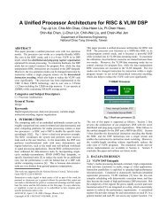
Figure 3.1 shows an example, comparing the result of the standard Hough technique
and our improved Hough technique. Figure 3.1èaè shows a synthesized image without noise.
It contains roughly 40 segments. Figure 3.1èbè shows the result of the standard Hough
analysis. 50 lines are detected. 17 true lines are missing. Also many of the true lines are
detected multiple times. Figure 3.1ècè shows the result by applying our improved Hough
technique without enhancement of using proximity grouping. Also, 50 lines are detected.
There is no missing true lines. Yet, since more lines are detected than are actually present
in the source image, a few true lines are detected multiple times. Figure 3.1èdè shows the
result by applying our improved Hough technique with proximity grouping enhancement.
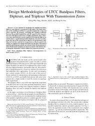
Figure 3.2èaè shows the same image as in Figure 3.1èaè, yet with serious noise. Figure
3.2èbè to Figure 3.2èdè are the correspondences of Figure 3.1èbè to Figure 3.1èdè . The
performance improvement over the standard Hough technique is much obvious.
3.3 Implementation and Measured Performance
In our implementation, we use æç = 1 è1 degreeè and ær = 1 è1 pixelè as the quantization
values for ç and r in Hough space. This appears quite suæcient for our subsequent applications.
Intuitively, smaller values of æç might give better precision but can result in the
spreading of peaks èrecall that image is digitized so that the edgels of a line will not lie

CHAPTER 3. NOISE IN THE HOUGH TRANSFORM 28
èaè A test image without noise. It contains
roughly 40 segments.
èbè 50 lines are detected using the
standard Hough transform.
ècè 50 lines are detected using our
improved Hough transform without
proximity grouping.
èdè 50 lines are detected using our improved
Hough transform with proximity
grouping.
Figure 3.1: A comparison of the results of the standard Hough technique and our improved
Hough technique, when applied to an image without noise.

CHAPTER 3. NOISE IN THE HOUGH TRANSFORM 29
èaè A test image with serious noise. It
contains roughly 40 segments.
èbè 50 lines are detected using the
standard Hough transform.
ècè 50 lines are detected using our
improved Hough transform without
proximity grouping.
èdè 50 lines are detected using our improved
Hough transform with proximity
grouping.
Figure 3.2: A comparison of the results of the standard Hough technique and our improved
Hough technique, when applied to a noisy image.

CHAPTER 3. NOISE IN THE HOUGH TRANSFORM 30
precisely on a digitized line except when the line has orientation of 0 æ ,45 æ ,90 æ or 135 æ è.
Similarly smaller values of ær give better precision but result in the spreading of peaks.
We have performed a series of experiments on synthesized images containing polygonal
objects, which are arbitrarily chosen from our model base èsee Figure 3.3è. èThe same
images are used in our later experiments.è
model-0 model-1 model-2 model-3 model-4
model-5 model-6 model-7 model-8 model-9
model-10 model-11 model-12 model-13 model-14
model-15 model-16 model-17 model-18 model-19
Figure 3.3: The twenty models used in our experiments. From left to right, top to bottom
are model-0 to model-19.
Two kinds of noise are imposed in our experiments: positive and negative.

CHAPTER 3. NOISE IN THE HOUGH TRANSFORM 31
We generate negative noise by randomly erasing edgels from the object boundary. For
example, if we want 10è of the boundary to be missing èoccludedè, we scan along the
boundary of every object and erase the edgels whenever ran modulo 10 = 0, where ran
is a random number; similarly, ifwewant 20è of the boundary to be missing, we dothe
same whenever ran modulo 5 = 0.
The positive noise we generate consists of random dot noise and segment noise. Random
dot noise is an additive dot noise whose position in the image is randomly selected; segment
noise is added by randomly selecting a position in the image and an orientation èfrom 0 æ
to 360 æ è for the segment then putting a line segment of length varying randomly from 0
to 7 pixels.
Simulations consider diæerent combinations of noise levels. The image size used in our
experiments is 256 æ 256. Figure 3.4 shows a sample scene èimage-0è after application of
various noise levels. Other test images are shown in Figure 3.5. The same noise levels were
applied to them.
In the following, we show the result of experiments on ten images. The number of lines
we select is 70. Since more lines are detected than are actually present in the source image,
our experiments allow for spurious lines.
The following abbreviated table shows lines by the ranks of their votes, using ë*" to
represent lines actually present in the source image and ë." to represent spurious lines.
Standard deviations of the ç and r values and their covariances are also given; this data is
of signiæcance for design of the later recognition stage.
æ case 0: no noise imposed on the image
image-0: *************************************************.****.*..***.........
image-1: ******************************.*******************.**...*..*....**....
image-2: ********************************************************.*..**.*..*...
image-3: *************************************************......*.........*....
image-4: ****************.**********.****************.********...*..**.........
image-5: **********************************************.***.*...........*..*.*.
image-6: ***********************************************************.*.*..*....
image-7: ******************************************************.****...........
image-8: ***************************************************.**.*..*.....*...*.
image-9: *********************************************..************.*.....*..*
ç ç = 1.398227 èdegreeè or 0.024404 èradianè; ç r = 1.672734 èpixelè;
ç çr = 0.189464 èdegree.pixelè or 0.003307 èradian.pixelè.
æ case 1: 10è negative noise, no positive noise

CHAPTER 3. NOISE IN THE HOUGH TRANSFORM 32
è0è Image-0 with no noise è1è Image-0 with 10è
negative noise and no positive
noise
è2è Image-0 with 10è
negative noise and 200
pieces of positive noise
è3è Image-0 with 10è
negative noise and 400
pieces of positive noise
è4è Image-0 with 10è
negative noise and 800
pieces of positive noise
è5è Image-0 with 20è
negative noise and no positive
noise
è6è Image-0 with 20è
negative noise and 200
pieces of positive noise
è7è Image-0 with 20è
negative noise and 400
pieces of positive noise
è8è Image-0 with 20è
negative noise and 800
pieces of positive noise
Figure 3.4: Reading from top to bottom, left to right, è0è to è8è are image-0 with diæerent
noise levels corresponding to cases 0 to 8.

CHAPTER 3. NOISE IN THE HOUGH TRANSFORM 33
Image-1 Image-2 Image-3
Image-4 Image-5 Image-6
Image-7 Image-8 Image-9
Figure 3.5: Image-1 to Image-9 before noise is imposed. The same noise levels as for
Image-0 are applied during our experiments.

CHAPTER 3. NOISE IN THE HOUGH TRANSFORM 34
image-0: **********************************************.*.***.*.*..............
image-1: ***************************************.***.****.....*.**...*.....*...
image-2: *********************************************************..*..*.......
image-3: **************************************.*******...***.*...*.*.......*..
image-4: ****************.*.***************..***.*..**.*.*.*............*...*..
image-5: ***************************************************.....*.*.*.**.....*
image-6: ************************************************************..........
image-7: ****************************************************.****....*.*......
image-8: ****************************************************.*...*.*.*..*.....
image-9: ***********************************..***********************.*......*.
ç ç = 1.496886 èdegreeè or 0.026126 èradianè; ç r = 1.803655 èpixelè;
ç çr = 0.244846 èdegree.pixelè or 0.004273 èradian.pixelè.
æ case 2: 10è negative noise, along with 200 pieces of random dot noise and 200 pieces
of segment noise
image-0: ******************************.******.*.*........*..*..........*......
image-1: ***********************.*.******.********..**..*.*............*.*.....
image-2: ***************************************.***.*.***.*...***.....*.......
image-3: *************************************.*****.*.*..*......*.....*.......
image-4: *****************.*********.****.*.*.*....**.*..**...*......*...*.....
image-5: **************************************.********.**.*.....*...*....***.
image-6: *********************************************.***.**.*.*..*..........*
image-7: ************************************************...**...**...*..***.*.
image-8: **************************************.**..***.*.*..*......*......*...
image-9: ******************************.*.*..********.***.*.*..*..*.......*.**.
ç ç = 1.656363 èdegreeè or 0.028909 èradianè; ç r = 2.059478 èpixelè;
ç çr = 0.119053 èdegree.pixelè or 0.002078 èradian.pixelè.
æ case 3: 10è negative noise, along with 400 pieces of random dot noise and 400 pieces
of segment noise
image-0: *****************.************..****.**......*.*.....*................
image-1: ***********************.*****..*********..**.......*...........*.....*
image-2: *********************************.*.***.***.*.***..........*........*.
image-3: *******************************.**..*.*..**...**.*.****..........**...
image-4: ****************.*********.*....****..*.*..*..*...............**....*.
image-5: *******************************.****.*.**..*.....*...*......*...*.**.*
image-6: *********************************.*.*****.*.*..**..........*..*.*....*
image-7: **********************************.*******.*****.**.....**.*......**..
image-8: **********************************...**.*..*.*.*......*...............
image-9: ***************************...*..*.*.**.*****.*.....*.......*........*
ç ç = 1.712783 èdegreeè or 0.029894 èradianè; ç r = 2.017484 èpixelè;
ç çr = 0.217823 èdegree.pixelè or 0.003802 èradian.pixelè.
æ case 4: 10è negative noise, along with 800 pieces of random dot noise and 800 pieces
of segment noise
image-0: *******************.***.***......****..*...*..........*..*.......*....
image-1: ****.**.**.**..*****.*.*..*.***.**.*....*..*.*....*..*..*.............
image-2: ***********.********.*..*...***..****.***.....*..............*.......*
image-3: *******.************.**.*.**.***...*....*.*..*.*......................
image-4: ************.*******....*.......*..******..*.............*....*....*..
image-5: ***************.***********.***......**..*........*............*......
image-6: ***************..*************..****..**.*..........*......*.........*
image-7: **************.***.*****.*****..***********.*.*...**..*...**.*.*...*..

CHAPTER 3. NOISE IN THE HOUGH TRANSFORM 35
image-8: ***************.********.****..***.*.****.*.*.....*..*................
image-9: ***********.**********.****..*.**...*.*..****.**.*..*...*..*...**.....
ç ç = 1.938883 èdegreeè or 0.033840 èradianè; ç r = 2.519878 èpixelè;
ç çr = -0.357589 èdegree.pixelè or -0.006241 èradian.pixelè.
æ case 5: 20è negative noise, along with no positive noise
image-0: ***********************************************.***...................
image-1: ********************************.***..******.**.*.*....**........*...*
image-2: ****************************************.***********.*..*.*....*......
image-3: ********************************.******.*.***..*.....**.*...*.*.*...*.
image-4: *********************.****.**.*****.**.******.**.*...........**...*...
image-5: ********************************************..*.....*.**.....*........
image-6: **********************************************************.*..*.......
image-7: ************************************.***************.*.*.*..*......*..
image-8: **********************************************.*.......*........*.....
image-9: ******************.*.******.********.*.*..*******.***.**.*.*.*..*.*...
ç ç = 1.563745 èdegreeè or 0.027293 èradianè; ç r = 1.913004 èpixelè;
ç çr = 0.219434 èdegree.pixelè or 0.003830 èradian.pixelè.
æ case 6: 20è negative noise, along with 200 pieces of random dot noise and 200 pieces
of segment noise
image-0: *************.****************.*..**.*.*.*.*..*......................*
image-1: ******************************.*..***...**..**.*...........*.....*..*.
image-2: ****************************.*****.*.**.**.......**.....****.*........
image-3: **************************************.**.***.***.....*.......*...*...
image-4: *******************.****.***..**.***...***..........................*.
image-5: ***********************************.*.**.***..*....................*..
image-6: **********************.***************..***...**.*..*...**.....*.*.*.*
image-7: ******************************.****..***...****.*..*...*..*..*.*......
image-8: *********************************.**..*.**.***.*..........*...........
image-9: ***********.*****.*.******.**.*****...*...***......*......*..*.*.**.*.
ç ç = 1.754688 èdegreeè or 0.030625 èradianè; ç r = 2.144938 èpixelè;
ç çr = 0.349338 èdegree.pixelè or 0.006097 èradian.pixelè.
æ case 7: 20è negative noise, along with 400 pieces of random dot noise and 400 pieces
of segment noise
image-0: *********.*****************.*.***.*...*.......*...*............*....*.
image-1: **********************.*.**..**.*****..*.*.*****......................
image-2: *******************.**.*****..*...*.**.*....*..**.....................
image-3: ***************************.**.*.**......*.........**...*........*....
image-4: ******************..**..*..**..*****..**...*.*............*.*.........
image-5: *****************.************.**.*........***.*............*........*
image-6: **********************..*******.*********.......*.**....*.***..*..*...
image-7: ****************************.*.*.***.*.***..........**.*.*....*.**....
image-8: *********************..*******.*.*****.*..*..**...*..*.......*..*.....
image-9: ***************..*.**.*.*.***.**.**..****....*.*.*........*...*.*.....
ç ç = 1.880869 èdegreeè or 0.032827 èradianè; ç r = 2.397261 èpixelè;
ç çr = -0.113044 èdegree.pixelè or -0.001973 èradian.pixelè.
æ case 8: 20è negative noise, along with 800 pieces of random dot noise and 800 pieces

CHAPTER 3. NOISE IN THE HOUGH TRANSFORM 36
of segment noise
image-0: ***********.****.******...*.****..*.....*.*...........**......*..*....
image-1: ***..**.***.**.**.***.**..*.*.*.*.**...*.*.*.....*....................
image-2: ******.*.****.**.**........***....**.....*........**.**.....*.........
image-3: **********.****.*..*****..*.*.*..**..*.*........*.*...............*..*
image-4: *************.*.*.*.......*.*..*.....*.........*..***...*.*.........**
image-5: ********.**********.*****...*...*....*.*........*..**...........**.*.*
image-6: ****************...*.*********...*....*.**...*....*.......*.*.....***.
image-7: *************.***.***.*..*.*.***.**.**.***.*...*.........*.**.......*.
image-8: ******.******....*.*****..*.....*.*.*.*...*.*.....*....*.............*
image-9: ********..*******..**..*....**.**.*******...*.....*......*.....**.....
ç ç = 2.168774 èdegreeè or 0.037852 èradianè; ç r = 2.503542 èpixelè;
ç çr = -0.396545 èdegree.pixelè or -0.006921 èradian.pixelè.
3.4 Some Additional Observations Concerning the Accuracy
of Hough Data
For the case when there is no noise imposed, we can see that true lines dominate the front
of the list èthose with high votesè and spurious lines are at the rear of the list. Note that
some of the true lines are detected multiply. This can happen when a line is slanting,
because its edgels become dispersed in ladder fashion,
and two parallel lines are often detected.
Negative noise is more devastating to the Hough transform than positive noise. Positive
noise, unless very intense, does not make true lines disappear; Negative noise subtracts
signals and can seriously aæect the accuracy of the line parameters detected. This is
especially true of short lines with a small slope. For example, given negative noise the edge
map
can turn into something like
or

CHAPTER 3. NOISE IN THE HOUGH TRANSFORM 37
Indeed, our experiments showed that most of the undetected lines are slanting lines with
small slopes.
While background subtraction works well to remove bias in favor of long line segments
over short line segments, it in fact implicitly applies the principle of the-winner-takes-all. In
particular, when a long line segment intersects a short line segment, their intersection pixel
will be classiæed as belonging to the long line segment and subtracted from the image after
the long line segment is detected. However, when these two line segments do not intersect
each other even though their extended lines do, the perceptual grouping technique we use
reduces this adverse eæect.
In regard to accuracy, we observe that line length is the key role aæecting the accuracy
of Hough transform results. The Hough transform works well to detect long line segments
even if the image is quite noisy. As line length decreases, noise aæects the accuracy of the
Hough transform even more seriously.
When the center of a segment is far away from the projection of the origin onto the
extended line of the segment, the average error of r increases. This phenomenon can be
rationalized as follows èsee Figure 3.6è: Since our algorithm loops through ç, we in fact
consider a line through the origin with slope angle ç èi.e., with line parameter èç +90 æ ; 0èè
and project all the image edgels onto this line. If bucket èç; rè in Hough space is detected
with n votes, roughly n edgels are projected onto the line at positions roughly r distant
from the origin. With this viewpoint in mind, due to the quantization of images, if the
center of a line segment, with line parameter èç; rè, is far away from the intersection point
of line èç; rè and line èç +90 æ ; 0è, the projections èonto line èç +90 æ ; 0èè of the points of
that line segment disperse èon line èç +90 æ ; 0èè around the position r distant from the
origin èexcept when the orientation of the line segment is0 æ ,45 æ ,90 æ or 135 æ .è

CHAPTER 3. NOISE IN THE HOUGH TRANSFORM 38
r
Projection of the Origin on the extended line
O
center of the segment
Figure 3.6: The thicker line is with parameter èç; rè. Projections of the pixels of this line
onto line èç +90 æ ;rè will disperse around the position r distant from the origin.

Chapter 4
Invariant Matching Using Line
Features
The idea behind the geometric hashing method is to encode local geometric features in a
manner which isinvariant under the geometric transformation that model objects undergo
during formation of the class of images being analyzed. This encoding can then be used in
a hash function that makes possible fast retrieval of model features from the hash table,
which can accordingly be viewed as an encoded model base. The technique can be applied
directly to line features, without resorting to point features indirectly derived from lines,
providing that we use some method of encoding line features in a way invariant under
transformations considered.
Potentially relevant transformation groups include rigid transformations, similarity
transformations, aæne transformations and projective transformations, depending on the
manner in which an image is formed. Each of these classes of transformations is a subgroup
of the full group of projective transformations. Since a projective transformation
is a collineation èreferring to p. 89 of ë35ëè, all these transformations preserve lines. This
allows us to use line features as inputs to the recognition procedures.
4.1 Change of Coordinates in Various Spaces
Since we will represent line features by their normal parameterization èç; rè, we show in
this section how the change of coordinates in image space by a linear transformation acts
39

CHAPTER 4. INVARIANT MATCHING USING LINE FEATURES 40
to change of coordinates in èç; rè-space. This is preliminary to the invariant line encodings
exploited in its following sections.
4.1.1 Change of Coordinates in Image Space
It is often easiest to work in homogeneous coordinates, since this allows projective transformations
to be represented by matrices.
Achange of coordinates in homogeneous coordinates is given by
w 0
= Tw;
where w = èw 1 ;w 2 ;w 3 è t is the homogeneous coordinate before transformation, w 0 =
èw 0 1 ;w0 2 3è t is the homogeneous coordinate after transformation and T is a non-singular
;w0
3 æ 3 matrix. Note that T and çT, for any ç 6= 0, deæne the same transformation, since
we are dealing with homogeneous coordinates.
A point èx; yè t in image space is represented by a non-zero 3-D point w =èw 1 ;w 2 ;w 3 è t
in homogeneous coordinate systems, such that
x = w 1
w 3
and y = w 2
w 3
;
where w 3 6=0. This representation is not unique, since çw, for any ç 6= 0 is also a
homogeneous representation of èx; yè t .
Every non-singular 3æ3 matrix deænes a 2-D projective transformation of homogeneous
coordinates.
Various subgroups of the projective transformation group are deæned by
diæerent restrictions on the form of the matrix T.
4.1.2 Change of Coordinates in Line Parameter Space
A line in a 2-D plane can be represented by its parameter vector and is usually parameterized
as
a 1 w 1 + a 2 w 2 + a 3 w 3 =0
or
a t w =0;
where a =èa 1 ;a 2 ;a 3 è t is the parameter vector of the line ènote that a 1 and a 2 are not both
equal to 0è and w =èw 1 ;w 2 ;w 3 è t is a homogeneous coordinate of any point on the line.

CHAPTER 4. INVARIANT MATCHING USING LINE FEATURES 41
This representation is not unique, since ça, for any ç 6= 0, is also a representation of the
same line.
A transformation T in image space changes the coordinate of every point w on a line
to w 0 by w 0 = Tw. Substituting w = T ,1 w 0 in a t w =0,we get
a t T ,1 w 0 =0
and hence
èèT ,1 è t aè t w 0 =0;
or
a 0 tw 0 =0; where a 0 =èT ,1 è t a:
This shows that the change of the coordinate of the point in3-D parameter space is
given by
a 0 = Pa:
where P =èT ,1 è t .
4.1.3 Change of Coordinates in èç; rè Space
Line features of an image are usually extracted by the Hough transform. A common
implementation of the Hough transform applies the normal parameterization suggested by
Duda and Hartë15ë, in the form
x cos ç + y sin ç = r;
where r is the perpendicular distance of the line to the origin and ç is the angle between
a normal to the line and the positive x-axis.
This unique parameterization of lines relates to the preceding parameterization of lines.
Let F : R 2 7! R 3 be a mapping such that
Fèèç; rè t è = ècos ç; sin ç; ,rè t
If we restrict the domain of ç to be in ë0;çè, then F ,1 exists. Deæne another mapping
G : R 3 7! R 2 by F ,1 as
Gèèa 1 ;a 2 ;a 3 è t è=
8
é
é:
F ,1 èèp 1
; p a 2
; p a 3
è t è
a 2 1 +a2 a
2
1 +a2 a
2
1 +a2 2
if a 2 ç 0
F ,1 èèp 1
; p ,a 2
; p ,a 3
è t è
a 2 1 +a2 a
2
1 +a2 a
2
1 +a2 2
otherwise

CHAPTER 4. INVARIANT MATCHING USING LINE FEATURES 42
where a 1 and a 2 are not both equal to 0. Then
Gèèa 1 ;a 2 ;a 3 è t è=
8
é
é:
ètan ,1 è a 2
è; p,a3
è t if a
a1 a 2 2 é 0
1 +a2 2
è0; ,a 3
a1 èt if a 2 =0
ètan ,1 è ,a 2
è; p
a3
è t if a
,a1 2 é 0
where the range of tan ,1 is in ë0::çè and tan ,1 è1è = ç 2 .
Then G maps a point a =èa 1 ;a 2 ;a 3 è t
a 2 1 +a2 2
both equal to 0, to èç; rè t = Gèaè inèç; rè-space such that
in parameter space, where a 1 and a 2 are not
a 1 w 1 + a 2 w 2 + a 3 w 3 =0
and
cos çw 1 + sin çw 2 , rw 3 =0
deæne the same line.
Let èç; rè t be the èç; rè-parameter deæning a line èin fact, the line x cos ç + y sin ç =
rè. Then Fèèç; rè t è=a, where a = ècos ç; sin ç; ,rè t ,isapoint in parameter space. A
transformation P changes the coordinate of a to a 0 = Pa in parameter space. Substituting
Fèèç; rè t è for a in a 0 = Pa, we get
a 0 = PFèèç; rè t è
and hence èç 0 ;r 0 è t = Gèa 0 è=GèPFèèç; rè t èè deænes the same line as a 0 èor ça 0 , ç 6= 0è.
Thus a transformation of a point in parameter space results in the transformation of
èç; rè t in èç; rè-space. The change of coordinate of èç; rè t in èç; rè-space is given by
èç 0 ;r 0 è t = Hèèç; rè t è
è4:1è
where H = G æ P æ F. 1
4.2 Encoding Lines by a Basis of Lines
To apply the geometric hashing technique to line features, we need to encode the features
in a manner invariant under the transformation group considered. One way of encoding is
1 We abused the notation by using Pèvè to denote Pv èmatrix P multiplies vector vè. We will continue
to use Pèvè orPv interchangeably when no ambiguity occurs.

CHAPTER 4. INVARIANT MATCHING USING LINE FEATURES 43
to ænd a canonical basis and a transformation èin the transformation group under considerationè
that maps the basis to the canonical basis, then apply that transformation to the
line being encoded. For example, let T be a projective transformation that maps a basis
b to Tèbè. If P is the unique transformation such that Pèbè = b c and P 0 is the unique
transformation such that P 0 èTèbèè = b c , where b c is the chosen canonical basis, then we
have P = P 0 æ T and any other line l and its correspondence l 0
= Tèlè will be mapped to
Pèlè by P and P 0 èl 0 èby P 0
respectively. Since P 0 èl 0 è=P 0 èTèlèè = P 0 æ Tèlè =Pèlè, this
is an invariant encodingë25ë.
Various subgroups of the projective transformation group require diæerent bases. We
discuss them in the following section and give formulae for the corresponding invariants.
Throughout the following discussion, we represent a line by its normal parameterization
èç; rè with ç in ë0; çè and r in R. If the computed invariant èç 0 ;r 0 è has ç 0
not in ë0::çè, we
adjust it by adding ç or ,ç and adjust the value of r 0
by æipping its sign accordingly.
4.3 Line Invariants under Various Transformation Groups
4.3.1 Rigid Line Invariants
Any correspondence of two ordered pairs of non-parallel lines determines a rigid transformation
up to a 180 æ -rotation ambiguity, and this ambiguity can be broken if we know the
position of a third line during veriæcation.
One way to encode a third line in terms of a pair of non-parallel lines in a rigid-invariant
way is to ænd a transformation P which maps the ærst basis line to the x-axis and maps
the second basis line to such that its intersection with the ærst basis line is the origin, and
then apply P to the third line.
A rigid transformation T in image space has the form
0
T = @ R b
0 1
0
1
A = B
@
cos ç , sin ç b1
sin ç cos ç b2
0 0 1
where R is the rotation matrix and b, the translation vector. This corresponds to the
1
C
A ;

CHAPTER 4. INVARIANT MATCHING USING LINE FEATURES 44
parameter-space transformation P, deæned by èc.f. section 4.1.2è
so that
P =èT ,1 è t =
0
@ èR,1 è t 0
,b t èR ,1 è t 1
P ,1 = T t =
1 0
A = @ R 0
0
@ Rt 0
b t 1
1
A :
,b t R 1
1
A ;
è4.2è
Let a line be parameterized as x cos ç + y sin ç , r = 0 and let two additional basis lines
be represented by their parameters a 1 and a 2 , such that
which are to be mapped by P to
a 1 = ècos ç 1 ; sin ç 1 ; ,r 1 è t ;
a 2 = ècos ç 2 ; sin ç 2 ; ,r 2 è t ;
e 1 = ècos ç 2 ; sin ç 2 ; 0èt =è0; 1; 0è t ;
e 2 = ècos '; sin '; 0è t =èC; S; 0è t :
Note that ' is æxed, though unknown. In this way, P maps the ærst basis line to x-axis
èor, y = 0è and the intersection of the two basis lines to the origin.
Since ax + by + c = 0 and çax + çby + çc =0,ç 6= 0, represent the same line, we have
ç 1 Pa 1 = e 1 ;
ç 2 Pa 2 = e 2 ;
where ç 1 and ç 2 are non-zero constants. Equivalently,
Then
Pèç 1 a 1 ;ç 2 a 2 è=èe 1 ; e 2 è:
èç 1 a 1 ;ç 2 a 2 è = P ,1 èe 1 ; e 2 è
=
=
0
B
@
0
B
@
cos ç sin ç 0
, sin ç cos ç 0
1 0
C
A
B
@
0 C
1 S
1
C
A
b 1 b 2 1 0 0
1
sin ç C cos ç + S sin ç
cos ç ,C sin ç + S cos ç C
A :
b 2 Cb 1 + Sb 2

CHAPTER 4. INVARIANT MATCHING USING LINE FEATURES 45
Thus
ç 1 = sin ç
= cos ç
= b 2
; è4.3è
cos ç 1 sin ç 1 ,r 1
ç 2 =
From Eq. è4.4è, we obtain
C cos ç + S sin ç
cos ç 2
=
,C sin ç + S cos ç
sin ç 2
= Cb 1 + Sb 2
,r 2
: è4.4è
C = ç 2 cosèç 2 + çè; è4.5è
S = ç 2 sinèç 2 + çè; è4.6è
b 1 = ,ç 2r 2 , Sb 2
C
è4.7è
and from Eq. è4.3è, we have sin ç sin ç 1 = cos ç cos ç 1 and thus ç = ç 2 , ç 1 or ç = , ç 2 , ç 1.
When ç = ç 2 , ç 1,wehave ç 1 = 1 and b 2 = ,r 1 . Substituting them and Eq. è4.5è,
Eq. è4.6è in Eq. è4.7è, we have b 1
Eq. è4.2è we obtain
P =
= ,èr 2 , r 1 cosèç 1 , ç 2 èè= sinèç 1 , ç 2 è. Thus, from
0
1
sin ç 1 , cos ç 1 0
B
cos ç
@
1 sin ç 1 0 C
A
cscèç 1 , ç 2 èèr 2 sin ç 1 , r 1 sin ç 2 è cscèç 1 , ç 2 èè,r 2 cos ç 1 + r 1 cos ç 2 è 1
When ç = , ç 2 , ç 1,wehave ç 1 = ,1 and b 2 = r 1 . Substituting them and Eq. è4.5è,
Eq. è4.6è in Eq. è4.7è, we have b 1 =èr 2 , r 1 cosèç 1 , ç 2 èè= sinèç 1 , ç 2 è. Thus, from Eq. è4.2è
we obtain
P =
0
1
, sin ç 1 cos ç 1 0
B
@
, cos ç 1 , sin ç 1 0 C
A
cscèç 1 , ç 2 èèr 2 sin ç 1 , r 1 sin ç 2 è cscèç 1 , ç 2 èè,r 2 cos ç 1 + r 1 cos ç 2 è 1
From section 4.1.3, the invariant èç 0 ;r 0 è t of a line èç; rè t can be obtained from the basis
lines as follows
èç 0 ;r 0 è t = Hèèç; rè t è=GèPècos ç; sin ç;,rè t è=Gèa 0 è
where
a 0 =
0
B
@
, sinèç , ç 1 è
cosèç , ç 1 è
,r , r 2 cscèç 1 , ç 2 è sinèç , ç 1 è+r 1 cscèç 1 , ç 2 è sinèç , ç 2 è
1
C
A ;

CHAPTER 4. INVARIANT MATCHING USING LINE FEATURES 46
or
a 0 =
0
B
@
sinèç , ç1è
, cosèç , ç1è
,r , r2 cscèç1 , ç2è sinèç , ç1è+r1 cscèç1 , ç2è sinèç , ç2è
1
C
A ;
depending upon which P is used, and hence
ç 0 = tan ,1 è cosèç , ç 1è
, sinèç , ç1è è = tan,1 è sinèç , ç 1 + ç 2 è
cosèç , ç1 + ç 2 èè=ç , ç 1 + ç 2 ;
r 0 = r + r2 cscèç1 , ç2è sinèç , ç1è , r1 cscèç1 , ç2è sinèç , ç2è;
or
ç 0 = tan ,1 è , cosèç , ç 1è
sinèç , ç1è è = tan,1 è sinèç , ç 1 , ç 2 è
cosèç , ç1 , ç 2 èè=ç , ç 1 , ç 2 ;
r 0 = r + r2 cscèç1 , ç2è sinèç , ç1è , r1 cscèç1 , ç2è sinèç , ç2è:
We may store each encoded invariant èç 0 ;r 0 è redundantly in two entries of the hash
table, èç 0 ;r 0 è and èç 0 ; ,r 0 è, during preprocessing. Then we may hit a match with either
èç 0 ;r 0 èorèç 0 ; ,r 0 è as the computed scene invariant during recognition. èNote that with
180 o -rotation, the computed invariants should be èç; rè and èç + ç; rè. However, we would
like to restrict ç to be in ë0::çè, which makes the invariants to be èç; rè and èç;,rè, where
ç is in ë0::çè.è
4.3.2 Similarity Line Invariants
To determine a similarity transformation uniquely, we need a correspondence of a pair of
triplets of lines, not all of which are parallel to each other or intersect at a common point.
Without loss of generality, wemay assume that the ærst basis line intersects the other
two basis lines. One way to encode a fourth line in a similarity-invariant way is to ænd a
transformation P which maps the ærst basis line to the x-axis, maps the second basis line
to such that its intersection with the ærst basis line is the origin and maps the third basis
line to such that its intersection with the ærst basis line has Euclidean coordinate è1; 0è,
and then apply P to the fourth line.

CHAPTER 4. INVARIANT MATCHING USING LINE FEATURES 47
A similarity transformation T in image space has the form
T =
0
@ s R
b
0 1
0
1
A = B
@
s cos ç ,s sin ç b 1
s sin ç s cos ç b 2
0 0 1
1
C
A ;
where s is the scaling factor; R, the rotation matrix; b, the translation vector.
corresponds to the parameter-space transformation P, deæned by èc.f. section 4.1.2è
so that
P =èT ,1 è t =
0
@ 1 èR,1 è t s
0
, 1 s bt èR ,1 è t 1
P ,1 = T t =
1 0
A = @ 1 R 0
s
, 1 s bt R 1
0
@ sRt 0
b t 1
1
A :
1
A ;
This
è4.8è
Let a line be parameterized as x cos ç + y sin ç , r = 0 and let three additional basis lines,
assuming the ærst line is not parallel to the others, be represented by their parameters a 1 ,
a 2 and a 3 , such that
a 1 = ècos ç 1 ; sin ç 1 ; ,r 1 è t ;
a 2 = ècos ç 2 ; sin ç 2 ; ,r 2 è t ;
a 3 = ècos ç 3 ; sin ç 3 ; ,r 3 è t ;
which are to be mapped by P to
e 1 = ècos ç 2 ; sin ç 2 ; 0èt =è0; 1; 0è t ;
e 2 = ècos ' 1 ; sin ' 1 ; 0è t =èC 1 ;S 1 ; 0è t ;
e 3 = ècos ' 2 ; sin ' 2 ; , sin jç 1 , ç 3 jè t =èC 2 ;S 2 ; , sin jç 1 , ç 3 jè t :
Note that ' 1 and ' 2 are æxed, though unknown. Also note that since we æxed the third
component ofe 3 to be , sin jç 1 , ç 3 j é 0, ' 2 ranges within è, ç 2 ; ç 2 è èor, C 2 é 0è. In this
way, P maps the ærst basis line to x-axis; the intersection of the ærst basis line and the
second basis line to the origin; the intersection of the ærst basis line and the third basis
line to è1; 0è t .

CHAPTER 4. INVARIANT MATCHING USING LINE FEATURES 48
Since ax + by + c = 0 and çax + çby + çc =0,ç 6= 0, represent the same line, we have
ç 1 Pa 1 = e 1 ;
ç 2 Pa 2 = e 2 ;
ç 3 Pa 3 = e 3 ;
where ç 1 , ç 2 and ç 3 are non-zero constants. Equivalently,
Pèç 1 a 1 ;ç 2 a 2 ;ç 3 a 3 è=èe 1 ; e 2 ; e 3 è:
Then
èç 1 a 1 ;ç 2 a 2 ;ç 3 a 3 è=P ,1 èe 1 ; e 2 ; e 3 è
=
=
0
B
@
0
B
@
s cos ç s sin ç 0
,s sin ç s cos ç 0
b 1 b 2 1
1 0
C
A
B
@
0 C 1 C 2
1 S 1 S 2
0 0 , sin jç 1 , ç 3 j
s sin ç sC 1 cos ç + sS 1 sin ç sC 2 cos ç + sS 2 sin ç
s cos ç ,sC 1 sin ç + sS 1 cos ç ,sC 2 sin ç + sS 2 cos ç
b 2 C 1 b 1 + S 1 b 2 C 2 b 1 + S 2 b 2 , sin jç 1 , ç 3 j
1
C
A
1
C
A :
Thus
ç 1 = s sin ç
cos ç 1
= s cos ç
sin ç 1
= b 2
,r 1
; è4.9è
ç 2 = s èC 1 cos ç + S 1 sin çè
cos ç 2
= s è,C 1 sin ç + S 1 cos çè
sin ç 2
= C 1 b 1 + S 1 b 2
,r 2
; è4.10è
ç 3 = s èC 2 cos ç + S 2 sin çè
cos ç 3
= s è,C 2 sin ç + S 2 cos çè
sin ç 3
= C 2 b 1 + S 2 b 2 , sin jç 1 , ç 3 j
,r 3
: è4.11è

CHAPTER 4. INVARIANT MATCHING USING LINE FEATURES 49
From Eq. è4.9è, we have s sin ç sin ç 1 = s cos ç cos ç 1 and thus ç = ç 2 , ç 1 or ç = , ç 2 , ç 1.
From Eq. è4.10è, we obtain
From Eq. è4.11è, we obtain
C 1 = ç 2
s cosèç 2 + çè;
S 1 = ç 2
s sinèç 2 + çè;
b 1 = ,ç 2r 2 , S 1 b 2
C 1
: è4.12è
C 2 = ç 3
S 2 = ç 3
and since C 2 2 + S2 2 =1,wehave ç 3 = æs.
s cosèç 3 + çè;
s sinèç 3 + çè;
b 1 = ,ç 3r 3 , S 2 b 2 + sin jç 1 , ç 3 j
C 2
; è4.13è
When ç = ç 2 , ç 1,wehave ç 1 = s and b 2 = ,sr 1 ; when ç = , ç 2 , ç 1,wehave ç 1 = ,s
and b 2 = sr 1 . In both cases, b 1 in Eq. è4.12è and Eq. è4.13è must be consistent, we can
solve toget
ç 3 =
sinèç 1 , ç 2 è sin jç 1 , ç 3 j
r 1 sinèç 2 , ç 3 è+r 2 sinèç 3 , ç 1 è+r 3 sinèç 1 , ç 2 è :
Since we require C 2 é 0, we have ç 3 = s when ç 1 éç 3 and ç = , ç 2 , ç 1 or ç 1 éç 3 and
ç = ç 2 , ç 1;wehave ç 3 = ,s when ç 1 éç 3 and ç = ç 2 , ç 1 or ç 1 éç 3 and ç = , ç 2 , ç 1.
To summarize, we have four cases as follows:
æ case 1 ç 1 éç 3 èthus sin jç 1 , ç 3 j = , sinèç 1 , ç 3 èè
í case 1.1
ç = ç 2 , ç 1;
s =
sinèç 1 , ç 2 è sinèç 1 , ç 3 è
r 1 sinèç 2 , ç 3 è+r 2 sinèç 3 , ç 1 è+r 3 sinèç 1 , ç 2 è ;
b 1 = s è,r 2 + r 1 cosèç 1 , ç 2 èè
sinèç 1 , ç 2 è
b 2 = ,sr 1 ;
;

CHAPTER 4. INVARIANT MATCHING USING LINE FEATURES 50
í case 1.2
ç = , ç 2 , ç 1;
s = ,
sinèç 1 , ç 2 è sinèç 1 , ç 3 è
r 1 sinèç 2 , ç 3 è+r 2 sinèç 3 , ç 1 è+r 3 sinèç 1 , ç 2 è ;
b 1 = , s è,r 2 + r 1 cosèç 1 , ç 2 èè
b 2 = sr 1 ;
sinèç 1 , ç 2 è
;
æ case 2 ç 1 éç 3 èthus sin jç 1 , ç 3 j = sinèç 1 , ç 3 èè
í case 2.1
ç = ç 2 , ç 1;
s =
sinèç 1 , ç 2 è sinèç 1 , ç 3 è
r 1 sinèç 2 , ç 3 è+r 2 sinèç 3 , ç 1 è+r 3 sinèç 1 , ç 2 è ;
b 1 = s è,r 2 + r 1 cosèç 1 , ç 2 èè
sinèç 1 , ç 2 è
b 2 = ,sr 1 ;
;
í case 2.2
ç = , ç 2 , ç 1;
s = ,
sinèç 1 , ç 2 è sinèç 1 , ç 3 è
r 1 sinèç 2 , ç 3 è+r 2 sinèç 3 , ç 1 è+r 3 sinèç 1 , ç 2 è ;
b 1 = , s è,r 2 + r 1 cosèç 1 , ç 2 èè
;
sinèç 1 , ç 2 è
b 2 = sr 1 :
Note that case 1.1 and case 2.1 are identical and case 1.2 and case 2.2 are identical.
The transformation P derived from case 1.1 and case 1.2 are again identical. We conclude
that the above four cases result in
P = 1 D
0
B
@
A sin ç 1 ,A cos ç 1 0
A cos ç 1 A sin ç 1 0
èr 2 sin ç 1 , r 1 sin ç 2 è sinèç 1 , ç 3 è ,èr 2 cos ç 1 , r 1 cos ç 2 è sinèç 1 , ç 3 è D
1
C
A

CHAPTER 4. INVARIANT MATCHING USING LINE FEATURES 51
where
A = r 1 sinèç 2 , ç 3 è+r 2 sinèç 3 , ç 1 è+r 3 sinèç 1 , ç 2 è;
D = sinèç 1 , ç 2 è sinèç 1 , ç 3 è:
From section 4.1.3, the invariant èç 0 ;r 0 è t of a line èç; rè t can be obtained from the basis
lines as follows
èç 0 ;r 0 è t = Hèèç; rè t è=GèPècos ç; sin ç;,rè t è=Gèa 0 è
where
a 0
= 1 D
0
B
@
,A sinèç , ç 1 è
A cosèç , ç 1 è
è,r 2 sinèç , ç 1 è+r 1 sinèç , ç 2 è , r sinèç 1 , ç 2 èè sinèç 1 , ç 3 è
1
C
A
and hence
ç 0 = tan ,1 è A cosèç , ç 1è
,A sinèç , ç 1 è è = tan,1 è sinèç , ç 1 + ç 2 è
cosèç , ç 1 + ç 2 è è=ç , ç 1 + ç 2 ;
r 0 = èr 2 sinèç , ç 1 è , r 1 sinèç , ç 2 è+r sinèç 1 , ç 2 èè sinèç 1 , ç 3 è=jAj:
4.3.3 Aæne Line Invariants
To determine an aæne transformation uniquely, we need a correspondence of two ordered
triplets of lines, which are not parallel to one another and do not intersect at a common
point.
One way to encode a fourth line in an aæne-invariant way is to ænd a transformation
P which maps the three basis lines to a canonical basis, say x =0,y = 0 and x + y =1,
and then apply P to the fourth line.
An aæne transformation T in image space has the form
T =
0
@ A
b
0 1
0
1
A = B
@
a 11 a 12 b 1
a 21 a 22 b 2
0 0 1
1
C
A ;
where A is the skewing matrix; b, the translation vector. This corresponds to the
parameter-space transformation P, deæned by èc.f. section 4.1.2è
P =èT ,1 è t =
0
@ èA,1 è t 0
,b t èA ,1 è t 1
1
A ;
è4.14è

CHAPTER 4. INVARIANT MATCHING USING LINE FEATURES 52
so that
P ,1 = T t =
0
@ At 0
b t 1
Let a line be parameterized as x cos ç + y sin ç , r = 0 and let three additional basis lines
1
A :
be represented by their parameters a 1 , a 2 and a 3 , such that
which are to be mapped by P to
a 1 = ècos ç1 ; sin ç 1 ; ,r 1è t ;
a 2 = ècos ç2 ; sin ç 2 ; ,r 2è t ;
a 3 = ècos ç3 ; sin ç 3 ; ,r 3è t ;
e 1 = ècos 0; sin 0; 0è t =è1; 0; 0è t ;
e 2 = ècos ç 2 ; sin ç 2 ; 0èt =è0; 1; 0è t ;
e 3 = ècos ç 4 ; sin ç ,1
p
4 ; è t =è 1 1 ,1
p ; p ; p è t :
2 2 2 2
In this way, P maps the ærst basis line to y-axis; the second basis line to x-axis; the third
basis line to x + y =1.
Since ax + by + c = 0 and çax + çby + çc =0,ç 6= 0, represent the same line, we have
ç1Pa 1 = e 1 ;
ç2Pa 2 = e 2 ;
ç3Pa 3 = e 3 ;
where ç1, ç2 and ç3 are non-zero constants. Equivalently,
Then
Pèç1a 1 ;ç2a 2 ;ç3a 3 è=èe 1 ; e 2 ; e 3 è:
èç1a 1 ;ç2a 2 ;ç3a 3 è = P ,1 èe 1 ; e 2 ; e 3 è
=
=
0
B
@
0
B
@
a11 a21 0
a12 a22 0
b1 b2 1
a11
a12
b1
a21
a22
b2
1 0
C
A
B
@
1
1 0
1p
2
0 1
1p 2
C
A
0 0 , p 1
2
p1
èa11 + a21è
2
p1
2
èa12 + a22è
p1
èb1 + b2 2
, 1è
1
C
A :

CHAPTER 4. INVARIANT MATCHING USING LINE FEATURES 53
Thus
ç1 =
ç2 =
ç3 =
a11
cos ç1
From Eq. è4.15è, we obtain
= a 12
sin ç1
= b 1
; è4.15è
,r1
a21
= a 22
= b 2
; è4.16è
cos ç2 sin ç2 ,r2
p1
èa11 + a21è p1
èa12 + a22è
1p èb1 + b2 2 2 2
, 1è
=
=
: è4.17è
cos ç3
sin ç3 ,r3
a11 = ç1 cos ç1 ; a 12 = ç1 sin ç1 and b1 = ,ç1 r 1 : è4.18è
From Eq. è4.16è, we obtain
a21 = ç2 cos ç2 ; a 22 = ç2 sin ç2 and b2 = ,ç2 r 2 : è4.19è
From Eq. è4.17è, we obtain
a11 + a21 = ç3
p
2 cos ç3 ; a 12 + a22 = ç3
Substituting Eq. è4.18è and Eq. è4.19è into Eq. è4.20è, we have
and hence
ç1 cos ç1 + ç2 cos ç2 , ç3
ç1 sin ç1 + ç2 sin ç2 , ç3
p
p
2 sin ç3 and b1 + b2 , 1=,ç3 2 r3 : è4.20è
p
p
ç1 r 1 + ç2 r 2 , ç3
2 cos ç3 = 0;
2 sin ç3 = 0;
p
2 r3 = ,1;
ç1 = , sinèç2 , ç3è=èr1 sinèç2 , ç3è+r2 sinèç3 , ç1è+r3 sinèç1 , ç2èè;
ç2 = , sinèç3 , ç1è=èr1 sinèç2 , ç3è+r2 sinèç3 , ç1è+r3 sinèç1 , ç2èè:
Substituting ç1 and ç2 back to Eq. è4.18è and Eq. è4.19è, we immediately obtain,
a11 = , cos ç1 sinèç2 , ç3è=èr1 sinèç2 , ç3è+r2 sinèç3 , ç1è +r3 sinèç1 , ç2èè;
a12 = , sin ç1 sinèç2 , ç3è=èr1 sinèç2 , ç3è+r2 sinèç3 , ç1è +r3 sinèç1 , ç2èè;
a21 = , cos ç2 sinèç3 , ç1è=èr1 sinèç2 , ç3è+r2 sinèç3 , ç1è +r3 sinèç1 , ç2èè;
a22 = , sin ç2 sinèç3 , ç1è=èr1 sinèç2 , ç3è+r2 sinèç3 , ç1è +r3 sinèç1 , ç2èè;
b1 = r1 sinèç2 , ç3è=èr1 sinèç2 , ç3è +r2 sinèç3 , ç1è+r3 sinèç1 , ç2èè;
b2 = r2 sinèç3 , ç1è=èr1 sinèç2 , ç3è +r2 sinèç3 , ç1è+r3 sinèç1 , ç2èè:

CHAPTER 4. INVARIANT MATCHING USING LINE FEATURES 54
Thus the transformation P in parameter space can be obtained from Eq. è4.14è as
P =
where
0
B@
A cscèç 1 , ç 2 è cscèç 2 , ç 3 è sin ç 2 ,A cscèç 1 , ç 2 è cscèç 2 , ç 3 è cos ç 2 0
A cscèç 1 , ç 2 è cscèç 1 , ç 3 è sin ç 1 ,A cscèç 1 , ç 2 è cscèç 1 , ç 3 è cos ç 1 0
cscèç 1 , ç 2 èèr 2 sin ç 1 , r 1 sin ç 2 è , cscèç 1 , ç 2 èèr 2 cos ç 1 , r 1 cos ç 2 è 1
A = r 1 sinèç 2 , ç 3 è+r 2 sinèç 3 , ç 1 è+r 3 sinèç 1 , ç 2 è:
From section 4.1.3, the invariant èç 0 ;r 0 è t of a line èç; rè t can be obtained from the basis
lines as follows:
1
CA
3æ3
èç 0 ;r 0 è t = Hèèç; rè t è=GèPècos ç; sin ç;,rè t è=Gèa 0 è;
where
0
, cscèç 1 , ç 2 è cscèç 2 , ç 3 è sinèç , ç 2 è
1
èr 3 sinèç 1 , ç 2 è+r 2 sinèç 3 , ç 1 è+r 1 sinèç 2 , ç 3 èè
a 0 =
, cscèç 1 , ç 2 è cscèç 1 , ç 3 è sinèç , ç 1 è
B@
èr 3 sinèç 1 , ç 2 è+r 2 sinèç 3 , ç 1 è+r 1 sinèç 2 , ç 3 èè
CA
r 1 cscèç 1 , ç 2 è sinèç , ç 2 è , r 2 cscèç 1 , ç 2 è sinèç , ç 1 è , r
3æ1
and hence
ç 0 = tan ,1 èA cscèç 1 , ç 3 è sinèç 1 , çè cscèç 1 , ç 2 è=
A cscèç 2 , ç 3 è sinèç 2 , çè cscèç 1 , ç 2 èè;
è4.21è
r 0 = 1 ç èr 1 cscèç 1 , ç 2 è sinèç 2 , çè , r 2 cscèç 1 , ç 2 è sinèç 1 , çè +rè; è4.22è
where
ç =
q
csc 2 èç 1 , ç 3 è sin 2 èç 1 , çè + csc 2 èç 2 , ç 3 è sin 2 èç 2 , çè jA cscèç 1 , ç 2 èj;
A = r 1 sinèç 2 , ç 3 è+r 2 sinèç 3 , ç 1 è+r 3 sinèç 1 , ç 2 è:

CHAPTER 4. INVARIANT MATCHING USING LINE FEATURES 55
4.3.4 Projective Line Invariants
Although a projective transformation is fractional linear, one can well treat it as a linear
transformation by using homogeneous coordinates.
To determine a projective transformation uniquely, we need a correspondence of two
ordered quadruplets of lines and for each quadruplet, no three lines are parallel to one
another or intersect at a common point èthus no three points are collinear in parameter
spaceè.
One way to encode a æfth line in a projective-invariant way is to ænd a transformation
P which maps the four basis lines to a canonical basis, say x =0,y =0,x = 1 and y =1,
and then apply P to the æfth line.
A projective transformation T in image space has the form
0
1
a 11 a 12 a 13
T = B
a
@ 21 a 22 a 23 C
A :
a 31 a 32 a 33
This corresponds to the parameter-space transformation P, deæned by èc.f. section 4.1.2è
P =èT ,1 è t = 1 D
where
0
1
a 22 a 33 , a 23 a 32 a 23 a 31 , a 21 a 33 a 21 a 32 , a 22 a 31
B a
@ 13 a 32 , a 12 a 33 a 11 a 33 , a 13 a 31 a 12 a 31 , a 11 a 32 C
a 12 a 23 , a 13 a 22 a 13 a 21 , a 11 a 23 a 11 a 22 , a 12 a 21
D = a 11 a 22 a 33 + a 12 a 23 a 31 + a 13 a 21 a 32 , a 11 a 23 a 32 , a 12 a 21 a 33 , a 13 a 22 a 31 ;
so that
P ,1 = T t =
0
B
@
1
a 11 a 21 a 31
a 12 a 22 a 32 C
A :
a 13 a 23 a 33
A ;
è4.23è
Let a line be parameterized as x cos ç + y sin ç , r = 0 and let four additional basis lines
be represented by their parameters a 1 , a 2 , a 3 and a 4 , such that
a 1 = ècos ç 1 ; sin ç 1 ; ,r 1 è t ;
a 2 = ècos ç 2 ; sin ç 2 ; ,r 2 è t ;
a 3 = ècos ç 3 ; sin ç 3 ; ,r 3 è t ;
a 4 = ècos ç 4 ; sin ç 4 ; ,r 4 è t ;

CHAPTER 4. INVARIANT MATCHING USING LINE FEATURES 56
which are to be mapped by P to
e 1 = ècos 0; sin 0; 0è t =è1; 0; 0è t ;
e 2 = ècos ç 2 ; sin ç 2 ; 0èt =è0; 1; 0è t ;
e 3 = ècos 0; sin 0; ,1è t =è1; 0; ,1è t ;
e 4 = ècos ç 2 ; sin ç 2 ; ,1èt =è0; 1; ,1è t :
In this way, P maps the ærst basis line to y-axis; the second basis line to x-axis; the third
basis line to x = 1; the fourth basis line to y =1.
Since ax + by + c = 0 and çax + çby + çc =0,ç 6= 0, represent the same line, we have
ç1Pa 1 = e 1 ;
ç2Pa 2 = e 2 ;
ç3Pa 3 = e 3 ;
ç4Pa 4 = e 4 ;
where ç1, ç2, ç3 and ç4 are constants. Equivalently,
Pèç1a 1 ;ç2a 2 ;ç3a 3 ;ç4a 4 è=èe 1 ; e 2 ; e 3 ; e 4 è:
Then
We have
èç1a 1 ;ç2a 2 ;ç3a 3 ;ç4a 4 è = P ,1 èe 1 ; e 2 ; e 3 ; e 4 è
=
=
0
B
@
a11 a21 a31
a12 a22 a32
a13 a23 a33
1 0
C
A
B
@
1 0 1 0
0 1 0 1
0 0 ,1 ,1
0
1
a11 a21 a11 , a31 a21 , a31
B a12 a22 a12
@
, a32 a22 , a32 C
a13 a23 a13 , a33 a23 , a33
A :
1
C
A
ç1 =
ç2 =
a11
cos ç1
a21
cos ç2
ç3 = a 11 , a31
cos ç3
ç4 = a 21 , a31
cos ç4
= a 12
sin ç1
= a 22
sin ç2
= a 13
; è4.24è
,r1
= a 23
; è4.25è
,r2
= a 12 , a32
sin ç3
= a 22 , a32
sin ç4
= a 13 , a33
; è4.26è
,r3
= a 23 , a33
: è4.27è
,r4

CHAPTER 4. INVARIANT MATCHING USING LINE FEATURES 57
From Eq. è4.24è, we obtain
a 11 = ç 1 cos ç 1 ; a 12 = ç 1 sin ç 1 and a 13 = ,ç 1 r 1 : è4:28è
From Eq. è4.25è, we obtain
a 21 = ç 2 cos ç 2 ; a 22 = ç 2 sin ç 2 and a 23 = ,ç 2 r 2 : è4:29è
From Eq. è4.26è, we obtain
a 31 = a 11 , ç 3 cos ç 3 ; a 32 = a 12 , ç 3 sin ç 3 and a 33 = a 13 + ç 3 r 3 : è4:30è
From Eq. è4.27è, we obtain
a 31 = a 21 , ç 4 cos ç 4 ; a 32 = a 22 , ç 4 sin ç 4 and a 33 = a 23 + ç 4 r 4 : è4:31è
Since Eq. è4.30è and Eq. è4.31è must be consistent, we have by substituting Eq. è4.28è in
Eq. è4.30è and Eq. è4.29è in Eq. è4.31è,
ç 1 cos ç 1 , ç 2 cos ç 2 , ç 3 cos ç 3 = ,ç 4 cos ç 4 ;
ç 1 sin ç 1 , ç 2 sin ç 2 , ç 3 sin ç 3 = ,ç 4 sin ç 4 ;
ç 1 r 1 , ç 2 r 2 , ç 3 r 3 = ,ç 4 r 4 ;
and hence
where
ç 1 = C 1
C 4
ç 4 ; ç 2 = C 2
C 4
ç 4 and ç 3 = C 3
C 4
ç 4 ;
C 1 = ,r 4 sinèç 2 , ç 3 è+r 3 sinèç 2 , ç 4 è , r 2 sinèç 3 , ç 4 è;
C 2 = ,r 4 sinèç 1 , ç 3 è+r 3 sinèç 1 , ç 4 è , r 1 sinèç 3 , ç 4 è;
C 3 = r 4 sinèç 1 , ç 2 è , r 2 sinèç 1 , ç 4 è+r 1 sinèç 2 , ç 4 è;
C 4 = r 1 sinèç 2 , ç 3 è+r 2 sinèç 3 , ç 1 è+r 3 sinèç 1 , ç 2 è:
Thus
a 11 = cos ç 1
C 1
C 4
ç 4 ; a 12 = sin ç 1
C 1
C 4
ç 4 and a 13 = ,r 1
C 1
C 4
ç 4 ;
a 21 = cos ç 2
C 2
C 4
ç 4 ; a 22 = sin ç 2
C 2
C 4
ç 4 ; and a 23 = ,r 2
C 2
C 4
ç 4 ;

CHAPTER 4. INVARIANT MATCHING USING LINE FEATURES 58
a 31 = ècos ç 1
C 1
C 4
,cos ç 3
C 3
C 4
èç 4 ;a 32 = èsin ç 1
C 1
C 4
,sin ç 3
C 3
C 4
èç 4 and a 33 =è,r 1
C 1
C 4
+r 3
C 3
C 4
èç 4 :
The transformation P in parameter space can be obtained from Eq. è4.23è as
0
1
p 11 p 12 p 13
P = ,1=C 1 C 2 C 3 ç 4 B
p
@ 21 p 22 p 23 C
A
p 31 p 32 p 33
where
p 11 = C 2 èC 1 r 2 sin ç 1 , C 1 r 1 sin ç 2 + C 3 r 3 sin ç 2 , C 3 r 2 sin ç 3 è;
p 12 = ,C 2 èC 1 r 2 cos ç 1 , C 1 r 1 cos ç 2 + C 3 r 3 cos ç 2 , C 3 r 2 cos ç 3 è;
p 13 = C 2 èC 1 sinèç 1 , ç 2 è+C 3 sinèç 2 , ç 3 èè;
p 21 = C 1 C 3 èr 1 sin ç 3 , r 3 sin ç 1 è;
p 22 = ,C 1 C 3 èr 1 cos ç 3 , r 3 cos ç 1 è;
p 23 = ,C 1 C 3 sinèç 1 , ç 3 è;
p 31 = C 1 C 2 èr 1 sin ç 2 , r 2 sin ç 1 è;
p 32 = ,C 1 C 2 èr 1 cos ç 2 , r 2 cos ç 1 è;
p 33 = ,C 1 C 2 sinèç 1 , ç 2 è:
From section 4.1.3, the invariant èç 0 ;r 0 è t of a line èç; rè t can be obtained from the basis
lines as follows
èç 0 ;r 0 è t = Hèèç; rè t è=GèPècos ç; sin ç;,rè t è=Gèa 0 è
where
0
a 0 = ,1=C 1 C 2 C 3 ç 4
B
B
@
ABC
DEF
GCF
1
C
A
3æ1
where
A = èr 3 sinèç 1 , ç 2 è , r 2 sinèç 1 , ç 3 è+r 1 sinèç 2 , ç 3 èè;
B = èr 4 sinèç , ç 2 è , r 2 sinèç , ç 4 è+r sinèç 2 , ç 4 èè;
C = èr 4 sinèç 1 , ç 3 è , r 3 sinèç 1 , ç 4 è+r 1 sinèç 3 , ç 4 èè;

CHAPTER 4. INVARIANT MATCHING USING LINE FEATURES 59
D =
è,r 3 sinèç , ç 1 è+r 1 sinèç , ç 3 è , r sinèç 1 , ç 3 èè;
E = èr 4 sinèç 1 , ç 2 è , r 2 sinèç 1 , ç 4 è+r 1 sinèç 2 , ç 4 èè;
F = èr 4 sinèç 2 , ç 3 è , r 3 sinèç 2 , ç 4 è+r 2 sinèç 3 , ç 4 èè;
G = èr 2 sinèç , ç 1 è , r 1 sinèç , ç 2 è+r sinèç 1 , ç 2 èè;
and hence
ç 0 = tan ,1 èDEF=ABCè;
,GCF
r 0 = pèABCè 2 +èDEF è 2 :

Chapter 5
The Eæect of Noise on the
Invariants
In an environment aæected by serious noise and occlusion, line features are usually detected
using the Hough transform. However, detected line parameters èç; rè's always deviate
slightly from their true values, since in the physical process of image acquisition the
positions of the endpoints of a segment are usually randomly perturbed and occlusion also
aæects the process of the Hough transform. As long as a segment is not too short, this induces
only slight perturbation of the line parameters of the segment. Thus it is reasonable
for us to assume that detected line parameters diæer from the ëtrue" values by a small
perturbation having a Gaussian distribution.
In the following, we derive the ëspread" of the computed invariant over hash space
from the ëperturbation" of the lines which give rise to this invariant.
5.1 A Noise Model for Line Parameters
We make the following mild assumptions: The measured line parameters èç; rè's of a set
of lines
1. are statistically independent;
2. are distributed according to a Gaussian distribution centered at the true value of the
parameter;
60

CHAPTER 5. THE EFFECT OF NOISE ON THE INVARIANTS 61
3. have a æxed covariance æ =
0
@ ç2 ç
ç çr
ç çr
ç 2 r
1
A .
More precisely, let èç; rè be the ëtrue" value of the parameters of a line and èææ; æRè
be the stochastic variable denoting the perturbation of èç; rè. The joint probability density
function of ææ and æR is then given by
pèææ; æRè=
and is centered around èç; rè.
1
2ç p jæj expë,1 2 èææ; æRèæ,1 èææ; æRè t ë
5.2 The Spread Function of the Invariants
In the following, we derive, from the perturbations of the basis lines and the line being
encoded, a closed-form formula of the perturbation of the invariants considered in the
preceding chapter.
We ærst introduce a lemma and a corollary derived from the lemma.
Lemma: Let X 1 ;X 2 ; :::; X n have amultivariate Gaussian distribution with vector u of
means and positive deænite covariance matrix æ. Then the moment-generating function
of the multivariate Gaussian p:d:f: is given by
C =
æv
expëv t u + vt ë; for all real vectors of v:
2
0 1
@ c 11 ::: c 1n
A, a real 2æn matrix. Then the random variable Y is NèCu; CæCt è.
c 21 ::: c 2n
Corollary: Let Y t =èY 1 ;Y 2 è such that Y = CX, where X t =èX 1 ;X 2 ; :::; X n è and
Proof. The moment-generating function of the distribution Y is given by
Applying the above theorem, we have
Mèvè=Eèe vtY è=Eèe vt CX è=Eèe èCt vè tX è
vè
Mèvè = expëèC t vè t u + èCt t æèC t vè
ë
2
èCæC
= expëv t èCuè+ vt t èv
ë
2
Thus the random variable Y is NèCu; CæC t è.
Q.E.D.

CHAPTER 5. THE EFFECT OF NOISE ON THE INVARIANTS 62
Now, we go back to consider the perturbation of the invariant from the perturbation
of lines. In the preceding chapter, we have given formulae of the invariants èç 0 ;r 0 è's for
various transformations. These invariants are functions of the line being encoded, èç; rè t
and the basis lines, èç i ;r i è t :
i=1;...;k
èç 0 ;r 0 è t = fèèç; rè t ; èç 1 ;r 1 è t ; æææ; èç k ;r k è t è:
Equivalently we may rewrite the above equation as follows:
ç 0 = f 0 èèç; rè t ; èç 1 ;r 1 è t ; æææ; èç k ;r k è t è; è5.1è
r 0 = f 00 èèç; rè t ; èç 1 ;r 1 è t ; æææ; èç k ;r k è t è: è5.2è
The exact forms of Eq. è5.1è and Eq. è5.2è, together with the value of k èi.e., the number
of basis lines neededè, depend on the viewing transformation under consideration and are
given in section 4.3.1, 4.3.2, 4.3.3 and 4.3.4 respectively.
Introducing perturbations of the line parameters èç; rè t and èç i ;r i è t i=1;...;k
results in a
perturbation of the computed invariant èç 0 ;r 0 è t ,having the following form:
ç 0 + æç 0 = f 0 èèç + æç; r + ærè t ; èç 1 + æç 1 ;r 1 + ær 1 è t ; æææ; èç k + æç k ;r k + ær k è t è; è5.3è
r 0 + ær 0 = f 00 èèç + æç; r + ærè t ; èç 1 + æç 1 ;r 1 + ær 1 è t ; æææ; èç k + æç k ;r k + ær k è t è: è5.4è
Expanding Eq. è5.3è and Eq. è5.4è in Maclaurin series and ignoring second and higher
order perturbation terms and then subtracting Eq. è5.1è and Eq. è5.2è from them, we have
kX ç
æç 0 = @ç0 @ç0
@ç
ç
0
æç +
@ç @r ær + æç i + @ç0
ær i
@ç
i=1
i @r i
= c 11 æç + c 12 ær + c 13 æç 1 + c 14 ær 1 +...+c 1;2k+1æç k + c 1;2k+2ær k ; è5.5è
kX ç
ær 0 = @r0 @r0
@r
ç
0
æç +
@ç @r ær + æç i + @r0
ær i
@ç i @r i
i=1
= c 21 æç + c 22 ær + c 23 æç 1 + c 24 ær 1 +...+c 2;2k+1æç k + c 2;2k+2ær k ; è5.6è
where c 11 = @ç 0 =@ç, c 12 = @ç 0 =@r, c 21 = @r 0 =@ç, c 22 = @r 0 =@r, c 1;i = @ç 0 =@ç i,2,
c 2;i = @r 0 =@ç i,2, for i = 3; 5; ...; 2k + 1, and c 1;i = @ç 0 =@r i,2, c 2;i = @r 0 =@r i,2, for
i =4; 6; ...; 2k +2.
Let èææ; æRè, èææ i ; æR i è i=1;...;k and èææ 0 ; æR 0 è be stochastic variables denoting the
perturbations of èç; rè, èç i ;r i è i=1;...;k and èç 0 ;r 0 è respectively. Eq. è5.5è and Eq. è5.6è can

CHAPTER 5. THE EFFECT OF NOISE ON THE INVARIANTS 63
be rewritten as
ææ 0 = c 11 ææ + c 12 æR + c 13 ææ 1 + c 14 æR 1 +...+c 1;2k+1ææ k + c 1;2k+2æR k ;
æR 0 = c 21 ææ + c 22 æR + c 23 ææ 1 + c 24 æR 1 +...+c 2;2k+1ææ k + c 2;2k+2æR k :
Since pèææ; æRè and pèææ i ; æR i è i=1;...;k
are Gaussian and independent, we have that
p:d:f: pèææ; æR; ææ 1 ; æR 1 ; ...; ææ k ; æR k è is also Gaussian. More precisely,
pèææ; æR; ææ 1 ; æR 1 ; ...; ææ k ; æR k è
= pèææ; æRè pèææ 1 ; æR 1 è æææpèææ k ; æR k è
1
= è
è 1 expë, ^æ
è2çè
qj ,1 Vë
k+1 ^æj 2 Vt
where
V =
^æ =
0
èææ; æR; ææ 1 ; æR 1 ; ...; ææ k ; æR k è t
B@
ç 2 ç
ç çr ... ... 0 0
ç çr ç 2 0 0
r .
. ..
. .
.
..
. 0 0 ç 2 ç
ç çr
1
CA
Since
èææ 0 ; æR 0 è t =
0 0 ... ... ç çr ç 2 r
è2k+2èæè2k+2è:
0
@ c 11 c 12 ... c 1;2k+1 c 1;2k+2
c 21 c 22 ... c 2;2k+1 c 2;2k+2
1
A V;
from the above corollary, we can show that èææ 0 ; æR 0 è also has a Gaussian distribution
having p:d:f:
pèææ 0 ; æR 0 è=
and covariance matrix
2ç
1
p
jæ 1 expë, 0 j 2 èææ0 ; æR 0 èæ 0,1 èææ 0 ; æR 0 è t ë
æ 0 =
0
@ ç2 ç 0 ç ç 0 r 0
ç 0 0 ç r ç 2 r 0
1
A ;
è5.7è

CHAPTER 5. THE EFFECT OF NOISE ON THE INVARIANTS 64
where
ç 2 ç 0 = èc2 + 11 c2 + æææ+ 13 c2 1;2k+1 èç2 +èc2 + ç 12 c2 + æææ+ 14 c2 1;2k+2 èç2 + r 11 c 12 + c 13 c 14 + æææ+ c 1;2k+1 c 1;2k+2èç çr ;
ç 2 r 0 = èc2 21
+ c 2 23
+ æææ+ c 2 2;2k+1èç 2 +èc 2 ç 22
+ c 2 24
+ æææ+ c 2 2;2k+2èç 2 +
r 21 c 22 + c 23 c 24 + æææ+ c 2;2k+1 c 2;2k+2èç çr ;
ç ç
0 r
0 = èc 11 c 21 + c 13 c 23 + æææ+ c 1;2k+1 c 2;2k+1èç 2 +
ç 12 c 22 + c 14 c 24 + æææ+ c 1;2k+2 c 2;2k+2èç 2 +
r 11 c 22 + c 13 c 24 + æææ+ c 1;2k+1 c 2;2k+2 + c 21 c 12 + c 23 c 14 + æææ+ c 2;2k+1 c 1;2k+2èç çr :
Recall that in computing the invariant èç 0 ;r 0 è t ,wemay adjust the value of ç 0
by adding
ç or ,ç with the sign of r 0 æipped accordingly such that ç 0 is in ë0::çè. If this is the case,
then the covariance matrix æ 0 must be adjusted by æipping the sign of ç 0 ç r
0.
5.3 Spread Functions under Various Transformation Groups
In the following subsections, we specialize the general result derived in the preceding section
to the various transformation groups considered earlier.
5.3.1 Rigid-Invariant Spread Function
From section 4.3.1, we have two sets of invariants èdue to 180 o -rotation ambiguityè for
rigid transformations as follows:
and
ç 0 = ç , ç 1 + ç 2 ;
r 0 = r + cscèç 1 , ç 2èèr 2 sinèç , ç 1è , r 1 sinèç , ç 2èè;
ç 0 = ç , ç 1 , ç 2 ;
r 0 = r + cscèç 1 , ç2èèr 2 sinèç , ç 1è , r 1 sinèç , ç 2èè;
where èç; rè is the parameter of the line being encoded and èç i ;r i è i=1;2 are the parameters
of the basis lines.

CHAPTER 5. THE EFFECT OF NOISE ON THE INVARIANTS 65
Let èææ; æRè, èææ i ; æR i è i=1;2 and èææ 0 ; æR 0 è be stochastic variables denoting respectively
the perturbations of èç; rè, èç i
;r i
è i=1;2 and the computed invariant èç 0 ;r 0 è. From
section 5.2, we have
ææ 0 = c11ææ + c12æR + c13ææ1 + c14æR1 + c15ææ2 + c16æR2;
æR 0 = c21ææ + c22æR + c23ææ1 + c24æR1 + c25ææ2 + c26æR2:
Computing c i;j
's, we obtain,
c11 =1,
c12 =0, c22 =1,
c13 = ,1,
c14 =0,
c15 =0,
c16 =0,
c21 = cscèç1 , ç2èèr2 cosèç , ç1è , r1 cosèç , ç2èè,
c23 = , sinèç , ç2è csc 2 èç1 , ç2èèr2 , r1 cosèç1 , ç2èè,
c24 = , sinèç , ç2è cscèç1 , ç2è,
c25 = , sinèç , ç1è csc 2 èç1 , ç2èèr1 , r2 cosèç1 , ç2èè,
c26 = sinèç , ç1è cscèç1 , ç2è.
Thus we conclude that èææ 0 ; æR 0 è has a Gaussian distribution with p:d:f
and covariance matrix
pèææ 0 ; æR 0 è=
1
2ç
pjæj expë, 1 ; æR èæ ,1 0 èææ 0 ; æR 0 è t ë
2 èææ0
æ =
0
@ ç2 ç 0 ç ç 0 r 0
ç 0 0 ç r
ç 2 r 0
1
A ;
where
ç 2 ç 0 = 2ç2 ç ;
ç 2 r 0 = èc2 21 + c2 23 + c2 25 èç2 ç +è1+c2 24 + c2 26 èç2 r +2èc 21 + c23c24 + c25c26èç çr
;
ç ç
0 r
0 = èc21 , c23èç 2 ç +èc 22 , c24èç çr
:
5.3.2 Similarity-Invariant Spread Function
From section 4.3.2, we have the following formula for the invariant for similarity transformations:
ç 0 = = ç , ç1 + ç 2 ;
r 0 = sinèç1 , ç3è B=jAj

CHAPTER 5. THE EFFECT OF NOISE ON THE INVARIANTS 66
and
A = r 1 sinèç2 , ç3è+r2 sinèç3 , ç1è +r3 sinèç1 , ç2è;
B = r2 sinèç , ç1è , r1 sinèç , ç2è +r sinèç1 , ç2è;
where èç; rè is the parameter of the line being encoded and èç i ;r i è i=1;2;3 are the parameters
of the basis lines.
Let èææ; æRè, èææ i
; æR i
è i=1;2;3 and èææ 0 ; æR 0 è be stochastic variables denoting respectively
the perturbations of èç; rè, èç i
;r i
è i=1;2;3 and the computed invariant èç 0 ;r 0 è.
From section 5.2, we have
ææ 0 = c11ææ + c12æR + c13ææ1 + c14æR1 + c15ææ2 + c16æR2 + c17ææ3 + c18æR3;
æR 0 = c21ææ + c22æR + c23ææ1 + c24æR1 + c25ææ2 + c26æR2 + c27ææ3 + c28æR3:
Computing c i;j
's, we obtain,
c11 =1,
c12 =0,
c13 = ,1,
c14 =0,
c15 =0,
c16 =0,
c17 =0,
c18 =0,
c21 = r2 cosèç , ç1è , r1 cosèç , ç2è=jAj,
c22 = sinèç1 , ç2è=jAj,
c23 =ëèr2 cosèç1 , ç3è , r3 cosèç1 , ç2èèB=A,
r2 cosèç , ç1è +r cosèç1 , ç2èë=jAj,
c24 =ë, sinèç2 , ç3èB=A , sinèç , ç2èë=jAj,
c25 =ëèr3 cosèç1 , ç2è , r1 cosèç2 , ç3èèB=A+
r1 cosèç , ç2è , r cosèç1 , ç2èë=jAj,
c26 = ësinèç1 , ç3èB=A + sinèç , ç1èë=jAj,
c27 =èr1 cosèç2 , ç3è , r2 cosèç1 , ç3èèB=èAjAjè,
c28 = , sinèç1 , ç2èB=èAjAjè.
Thus we conclude that èææ 0 ; æR 0 è has a Gaussian distribution with p:d:f
pèææ 0 ; æR 0 è=
1
2ç
pjæj expë, 1 ; æR èæ ,1 0 èææ 0 ; æR 0 è t ë
2 èææ0
and covariance matrix
æ =
0
@ ç2 ç 0 ç ç 0 r 0
ç 0 0 ç r
ç 2 r 0
1
A ;

CHAPTER 5. THE EFFECT OF NOISE ON THE INVARIANTS 67
where
ç 2 ç 0 = 2ç2;
ç
ç 2 r 0 = èc2 21 + c2 23 + c2 25 + c2 27 èç2 +èc2 ç 22 + c2 24 + c2 26 + c2 28 èç2 + r
2èc21c22 + c23c24 + c25c26 + c27c28èç çr
;
ç ç
0 r
0 = èc21 , c23èç 2 ç +èc 22 , c24èç çr
:
5.3.3 Aæne-Invariant Spread Function
From section 4.3.3, the invariant for aæne transformations has the following form:
ç 0 = tan ,1 èA cscèç1 , ç3è sinèç1 , çè cscèç1 , ç2è=
r 0 = C=D
A cscèç2 , ç3è sinèç2 , çè cscèç1 , ç2èè;
and
A = r3 sinèç1 , ç2è +r2 sinèç3 , ç1è +r1 sinèç2 , ç3è;
B = csc 2 èç1 , ç3è sin 2 èç1 , ç4è + csc 2 èç2 , ç3è sin 2 èç2 , ç4è;
C = r1 cscèç1 , ç2è sinèç2 , çè , r2 cscèç1 , ç2è sinèç1 , çè +r;
q
D = A 2 B csc 2 èç1 , ç2è;
where èç; rè is the parameter of the line being encoded and èç i
;r i
è i=1;2;3 are the parameters
of the basis lines.
Let èææ; æRè, èææ i
; æR i
è i=1;2;3 and èææ 0 ; æR 0 è be stochastic variables denoting respectively
the perturbations of èç; rè, èç i
;r i
è i=1;2;3 and the computed invariant èç 0 ;r 0 è.
From section 5.2, we have
ææ 0 = c11ææ + c12æR + c13ææ1 + c14æR1 + c15ææ2 + c16æR2 + c17ææ3 + c18æR3;
æR 0 = c21ææ + c22æR + c23ææ1 + c24æR1 + c25ææ2 + c26æR2 + c27ææ3 + c28æR3:
Computing c i;j
's and writing E = cscèç1 , ç3è cscèç2 , ç3è=B, we obtain,
c11 = sinèç1 , ç2èE;
c12 = 0;

CHAPTER 5. THE EFFECT OF NOISE ON THE INVARIANTS 68
c 13 = , cscèç 1 , ç 3 è sinèç , ç 2 è sinèç , ç 3 èE;
c 14 = 0;
c 15 = cscèç 2 , ç 3 è sinèç , ç 1 è sinèç , ç 3 èE;
c 16 = 0;
c 17 = , cscèç 1 , ç 3 è cscèç 2 , ç 3 è sinèç 1 , ç 2 è sinèç , ç 1 è sinèç , ç 2 èE;
c 18 = 0;
c 21 = ë,ècosèç , ç 1 è csc 2 èç 1 , ç 3 è sinèç , ç 1 è+
cosèç , ç 2 è csc 2 èç 2 , ç 3 è sinèç , ç 2 èèC=B +
cscèç 1 , ç 2 èèr 2 cosèç , ç 1 è , r 1 cosèç , ç 2 èèë=D;
c 22 = 1=D;
c 23 = ë, cscèç 1 , ç 2 èèr 2 cosèç , ç 1 è + cotèç 1 , ç 2 èèr 2 sinèç , ç 1 è , r 1 sinèç , ç 2 èèè ,
Cèèr 3 cosèç 1 , ç 2 è , r 2 cosèç 1 , ç 3 èè=A ,
csc 2 èç 1 , ç 3 è sinèç , ç 1 èècosèç , ç 1 è + cotèç 1 , ç 3 è sinèç , ç 1 èè=Bè ,
cotèç 1 , ç 2 èë=D;
c 24 = ë, sinèç 2 , ç 3 èAC , cscèç 1 , ç 2 è sinèç , ç 2 èë=D;
c 25 = ëcscèç 1 , ç 2 èèr 1 cosèç , ç 2 è + cotèç 1 , ç 2 èèr 2 sinèç , ç 1 è , r 1 sinèç , ç 2 èèè ,
Cèèr 1 cosèç 2 , ç 3 è , r 3 cosèç 1 , ç 2 èè=A ,
csc 2 èç 2 , ç 3 è sinèç , ç 2 èècosèç , ç 2 è + cotèç 2 , ç 3 è sinèç , ç 2 èè=Bè +
cotèç 1 , ç 2 èë=D;
c 26 = ësinèç 1 , ç 3 èC=A + cscèç 1 , ç 2 è sinèç , ç 1 èë=D;
c 27 = ë,Cèèr 2 cosèç 1 , ç 3 è , r 1 cosèç 2 , ç 3 èè=A +
ècotèç 1 , ç 3 è csc 2 èç 1 , ç 3 è sin 2 èç , ç 1 è+
cotèç 2 , ç 3 è csc 2 èç 2 , ç 3 è sin 2 èç , ç 2 èè=Bèë=D;
c 28 = ë, sinèç 1 , ç 2 èC=Aë=D:
Thus we conclude that èææ 0 ; æR 0 è has a Gaussian distribution with p:d:f
pèææ 0 ; æR 0 è =
1
2ç p jæj expë, 1 2 èææ0 ; æR 0 èæ ,1 èææ 0 ; æR 0 è t ë
è5.8è

CHAPTER 5. THE EFFECT OF NOISE ON THE INVARIANTS 69
and covariance matrix
where
æ =
0
@ ç2 ç 0 ç ç 0 r 0
ç 0 0 ç r
ç 2 r 0
1
A ;
ç 2 ç 0 = èc2 11 + c 2 13 + c 2 15 + c 2 17èç 2 ; ç
ç 2 r 0 = èc2 21 + c2 23 + c2 25 + c2 27 èç2 +èc2 ç 22 + c2 24 + c2 26 + c2 28 èç2 + r
2èc21c22 + c23c24 + c25c26 + c27c28èç çr
;
ç 0 0 ç r
= èc11c21 + c13c23 + c15c25 + c17c27èç 2 ç
+èc11c22 + c13c24 + c15c26 + c17c28èç çr
:
5.3.4 Projective-Invariant Spread Function
From section 4.3.4, the invariant for projective transformations is as follows:
ç 0 = tan ,1 èDEF=ABCè;
,GCF
r 0 = p
èABCè 2 +èDEFè 2
and
A = èr3 sinèç1 , ç2è , r2 sinèç1 , ç3è+r1 sinèç2 , ç3èè;
B = èr4 sinèç , ç2è , r2 sinèç , ç4è+r sinèç2 , ç4èè;
C = èr4 sinèç1 , ç3è , r3 sinèç1 , ç4è+r1 sinèç3 , ç4èè;
D = è,r3 sinèç , ç1è+r1 sinèç , ç3è , r sinèç1 , ç3èè;
E = èr4 sinèç1 , ç2è , r2 sinèç1 , ç4è+r1 sinèç2 , ç4èè;
F = èr4 sinèç2 , ç3è , r3 sinèç2 , ç4è+r2 sinèç3 , ç4èè;
G = èr2 sinèç , ç1è , r1 sinèç , ç2è+r sinèç1 , ç2èè;
where èç; rè is the parameter of the line being encoded and èç i
;r i
è i=1;2;3;4 are the parameters
of the basis lines.
Let èææ; æRè, èææ i
; æR i
è i=1;2;3;4 and èææ 0 ; æR 0 è be stochastic variables denoting
respectively the perturbations of èç; rè, èç i
;r i
è i=1;2;3;4 and the computed invariant èç 0 ;r 0 è.
From section 5.2, we have
ææ 0 = c11ææ + c12æR + c13ææ1 + c14æR1 + c15ææ2 +

CHAPTER 5. THE EFFECT OF NOISE ON THE INVARIANTS 70
c 16 æR 2 + c 17 ææ 3 + c 18 æR 3 + c 19 ææ 4 + c 1;10 æR 4 ;
æR 0 = c 21 ææ + c 22 æR + c 23 ææ 1 + c 24 æR 1 + c 25 ææ 2 +
c 26 æR 2 + c 27 ææ 3 + c 28 æR 3 + c 29 ææ 4 + c 2;10 æR 4 :
Computing c i;j 's, we obtain,
c 11 = ëè,r 4 cosèç , ç 2 è+r 2 cosèç , ç 4 èèI=B +
è,r 3 cosèç , ç 1 è+r 1 cosèç , ç 3 èèEFë=HK;
c 12 = ësinèç 2 , ç 4 èI=B , sinèç 1 , ç 3 èEFë=HK;
c 13 = ë,èr 4 cosèç 1 , ç 3 è , r 3 cosèç 1 , ç 4 èèI=C +
èr 4 cosèç 1 , ç 2 è , r 2 cosèç 1 , ç 4 èèDF ,
èr 3 cosèç 1 , ç 2 è , r 2 cosèç 1 , ç 3 èèI=A +
èr 3 cosèç , ç 1 è , r cosèç 1 , ç 3 èèEFë=HK;
c 14 = ë, sinèç 3 , ç 4 èI=C + sinèç 2 , ç 4 èDF ,
sinèç 2 , ç 3 èI=A + sinèç , ç 3 èEFë=HK;
c 15 = ë,è,r 4 cosèç 2 , ç 3 è+r 3 cosèç 2 , ç 4 èèDE +
è,r 4 cosèç 1 , ç 2 è+r 1 cosèç 2 , ç 4 èèDF ,
è,r 4 cosèç , ç 2 è+r cosèç 2 , ç 4 èèI=B,
è,r 3 cosèç 1 , ç 2 è+r 1 cosèç 2 , ç 3 èèI=Aë=HK;
c 16 = ësinèç 3 , ç 4 èDE , sinèç 1 , ç 4 èDF +
sinèç , ç 4 èI=B + sinèç 1 , ç 3 èI=Aë=HK;
c 17 = ë,èr 4 cosèç 2 , ç 3 è , r 2 cosèç 3 , ç 4 èèDE +
èr 4 cosèç 1 , ç 3 è , r 1 cosèç 3 , ç 4 èèI=C,
èr 2 cosèç 1 , ç 3 è , r 1 cosèç 2 , ç 3 èèI=A +
è,r 1 cosèç , ç 3 è+r cosèç 1 , ç 3 èèEFë=HK;
c 18 = ë, sinèç 2 , ç 4 èDE + sinèç 1 , ç 4 èI=C ,
sinèç 1 , ç 2 èI=A , sinèç , ç 1 èEFë=HK;
c 19 = ë,è,r 3 cosèç 2 , ç 4 è+r 2 cosèç 3 , ç 4 èèDE +

CHAPTER 5. THE EFFECT OF NOISE ON THE INVARIANTS 71
è,r 3 cosèç 1 , ç 4 è+r 1 cosèç 3 , ç 4 èèI=C +
èr 2 cosèç 1 , ç 4 è , r 1 cosèç 2 , ç 4 èèDF ,
èr 2 cosèç , ç 4 è , r cosèç 2 , ç 4 èèI=Bë=HK;
c 1;10 = ësinèç 2 , ç 3 èDE , sinèç 1 , ç 3 èI=C +
sinèç 1 , ç 2 èDF , sinèç , ç 2 èI=Bë=HK;
c 21 = ëèr 4 cosèç , ç 2 è , r 2 cosèç , ç 4 èèHAC +
è,r 3 cosèç , ç 1 è+r 1 cosèç , ç 3 èèIEFëJ=L 3 +
ë,r 2 cosèç , ç 1 è+r 1 cosèç , ç 2 èëCF=L;
c 22 = ësinèç 2 , ç 4 èHAC , sinèç 1 , ç 3 èIEFëJ=L 3 ,
sinèç 1 , ç 2 èCF=L;
c 23 = ëèr 4 cosèç 1 , ç 3 è , r 3 cosèç 1 , ç 4 èèHAB +
èr 3 cosèç 1 , ç 2 è , r 2 cosèç 1 , ç 3 èèHBC +
èr 4 cosèç 1 , ç 2 è , r 2 cosèç 1 , ç 4 èèIDF +
èr 3 cosèç , ç 1 è+r cosèç 1 , ç 3 èèIEFëJ=L 3 ,
ër 4 cosèç 1 , ç 3 è , r 3 cosèç 1 , ç 4 èëGF=L +
ër 2 cosèç , ç 1 è , r cosèç 1 , ç 2 èëCF=L;
c 24 = ësinèç 3 , ç 4 èHAB + sinèç 2 , ç 3 èHBC +
sinèç 2 , ç 4 èIDF + sinèç , ç 3 èIEFëJ=L 3 ,
sinèç 3 , ç 4 èGF=L + sinèç , ç 2 èCF=L;
c 25 = ëè,r 4 cosèç , ç 2 è+r cosèç 2 , ç 4 èèHAC +
è,r 3 cosèç 1 , ç 2 è+r 1 cosèç 2 , ç 3 èèHBC +
èr 4 cosèç 2 , ç 3 è , r 3 cosèç 2 , ç 4 èèIDE,
èr 4 cosèç 1 , ç 2 è , r 1 cosèç 2 , ç 4 èèIDFëJ=L 3 ,
ër 4 cosèç 2 , ç 3 è , r 3 cosèç 2 , ç 4 èëGC=L +
ë,r 1 cosèç , ç 2 è+r cosèç 1 , ç 2 èëCF=L;
c 26 = ë, sinèç , ç 4 èHAC , sinèç 1 , ç 3 èHBC +
sinèç 3 , ç 4 èIDE, sinèç 1 , ç 4 èIDFëJ=L 3 ,
sinèç 3 , ç 4 èGC=L , sinèç , ç 1 èCF=L;

CHAPTER 5. THE EFFECT OF NOISE ON THE INVARIANTS 72
c 27 = ë,èr 4 cosèç 1 , ç 3 è , r 1 cosèç 3 , ç 4 èèHAB +
èr 2 cosèç 1 , ç 3 è , r 1 cosèç 2 , ç 3 èèHBC ,
èr 4 cosèç 2 , ç 3 è , r 2 cosèç 3 , ç 4 èèIDE +
è,r 1 cosèç , ç 3 è+r cosèç 1 , ç 3 èèIEFëJ=L 3 ,
ë,r 4 cosèç 2 , ç 3 è+r 2 cosèç 3 , ç 4 èëGC=L ,
ë,r 4 cosèç 1 , ç 3 è+r 1 cosèç 3 , ç 4 èëGF=L;
c 28 = ë, sinèç 1 , ç 4 èHAB + sinèç 1 , ç 2 èHBC ,
sinèç 2 , ç 4 èIDE, sinèç , ç 1 èIEFëJ=L 3 +
sinèç 2 , ç 4 èGC=L + sinèç 1 , ç 4 èGF=L;
c 29 = ëèr 3 cosèç 1 , ç 4 è , r 1 cosèç 3 , ç 4 èèHAB +
èr 2 cosèç , ç 4 è , r cosèç 2 , ç 4 èèHAC +
èr 3 cosèç 2 , ç 4 è , r 2 cosèç 3 , ç 4 èèIDE +
èr 2 cosèç 1 , ç 4 è , r 1 cosèç 2 , ç 4 èèIDFëJ=L 3 ,
ër 3 cosèç 2 , ç 4 è , r 2 cosèç 3 , ç 4 èëGC=L ,
ër 3 cosèç 1 , ç 4 è , r 1 cosèç 3 , ç 4 èëGF=L;
c 2;10 = ësinèç 1 , ç 3 èHAB + sinèç , ç 2 èHAC +
sinèç 2 , ç 3 èIDE + sinèç 1 , ç 2 èIDFëJ=L 3 ,
sinèç 2 , ç 3 èGC=L , sinèç 1 , ç 3 èGF=L:
and
H = ABC; I = DEF; J = GCF; K =è1+I 2 =H 2 è; L =
p
H 2 + I 2 :
Thus we conclude that èææ 0 ; æR 0 è has a Gaussian distribution with p:d:f
pèææ 0 ; æR 0 è=
1
2ç p jæj expë, 1 2 èææ0 ; æR 0 èæ ,1 èææ 0 ; æR 0 è t ë
and covariance matrix
æ =
0
@ ç2 ç 0 ç ç 0 r 0
ç 0 0 ç r
ç 2 r 0
1
A ;

CHAPTER 5. THE EFFECT OF NOISE ON THE INVARIANTS 73
where
ç 2 ç 0 = èc2 11 + c2 13 + æææ+ c2 19 èç2 ç +èc2 12 + c2 14 + æææ+ c2 1;10 èç2 r +
2èc11 c 12 + c13 c 14 + æææ+ c19 c 1;10èç çr
;
ç 2 r 0 = èc2 21 + c2 23 + æææ+ c2 29 èç2 ç +èc2 22 + c2 24 + æææ+ c2 2;10 èç2 r +
2èc21 c 22 + c23 c 24 + æææ+ c29 c 2;10èç çr
;
ç ç
0 r
0 = èc11 c 21 + c13 c 23 + æææ+ c19 c 29èç 2 ç +èc 12 c 22 + c14 c 24 + æææ+ c1;10 c 2;10èç 2 r +
èc11 c 22 + c13 c 24 + æææ+ c19 c 2;10 + c21 c 12 + c23 c 14 + æææ+ c29 c 1;10èç çr
:

Chapter 6
Bayesian Line Invariant Matching
Our recognition scheme builds upon the geometric hashing method, as reviewed in chapter
2, which also notes some weaknesses of the geometric hashing technique. Even when
we use an improved Hough transform to detect line features in a degraded image, we still
face the problem dealing with image noise and with the resulting problem of noise in the
invariants used for hashing.
To minimize these noise eæects, we need to derive a theoretically justiæed scheme for
weighted voting among hash bins. We show howaweighted voting scheme can be used to
cope with the problem. This is the aim of the probabilistic procedure which wenowgoon
to describe.
6.1 A Measure of Matching between Scene and Model Invariants
In the geometric hashing method described in chapter 2, during recognition a computed
scene invariant is used to index the geometric hash table and tally one vote for the entry
retrieved. However, considering the presence of noise, a scene invariant can not exactly
hit the hash table entry where its matching model invariant is supposed to reside. Gavrila
and Groen ë18ë assume a bounded circular region around each hash bin and tally equal
vote for all the bins within the region centered around the bin being hashed. However,
our analysis of the noise eæect on computed invariants in the preceding chapter shows
that the perturbation of an invariant has an approximately Gaussian distribution with a
74

CHAPTER 6. BAYESIAN LINE INVARIANT MATCHING 75
non-zero correlation coeæcient.
This implies that the region of hash space that would
need to be accessed is an ellipse, instead of a circle, centered around the ëtrue" value of
the invariant. Moreover, this perturbation also depends on the basis and the line being
encoded, which means that diæerent invariants should be associated with diæerent size,
shape and orientation of hash space regions for error tolerance.
The nodes in hash space that more ëclosely match" the value of the invariant should get
a higher weighted score than those which are far away, in a manner accurately representing
the behavior of the noise which aæects these invariants. Let inv s be a scene invariant and
let inv Mi be a model invariant computed from a basis B Mi and a line l j of M i . Bayes'
theorem ë16ë allows us to precisely determine the probability that inv s
presence of a certain ëM i ;B Mi ;l j ë:
where
P èëM i ;B Mi ;l j ëjinv s è = P èëM i ;B Mi ;l j ëè pèinv sjëM i ;B Mi ;l j ëè
pèinv s è
æ P èëM i ;B Mi ;l j ëè is the a priori probability that M i
B Mi
results from the
is embedded in the scene and
is selected to encode l j . We assume that all the models are equally likely to
appear and have the same number of features, which is a simpliæcation that could
be easily generalized. Thus P èëM i ;B Mi ;l j ëè is the same for all ëmodel, basis, lineë
combinations. èNote that this may not be quite true if the basis selection procedure
favors long bases instead of selecting bases randomly.è
æ pèinv s jëM i ;B Mi ;l j ëè is the conditional p:d:f: of observing inv s given that M i appears
in the scene with B Mi
being selected and l j being encoded. It consists of two parts:
the spike induced by ëM i ;B Mi ;l j ë and a background distribution.
æ pèinv s è is the p:d:f: of observing inv s , regardless of which ëM i ;B Mi ;l j ë induces it.
Assume that no twoinvariants of the same model and with a æxed basis locate near each
other in hash space èi.e., model features are distinct and separate; If more than one model
feature lands in approximately the same location, then the features should be coalesced
into a single featureè, inv s can be close to at most one model invariant. Thus, given inv s ,
the supporting evidence that M i appears in the scene and the basis B Mi is selected is then
P èëM i ;B Mi ëèjinv s è ç max P èëM i ;B Mi ;l j ëjinv s è
j

CHAPTER 6. BAYESIAN LINE INVARIANT MATCHING 76
è
max j pèinv s jëM i ;B Mi ;l j ëè
: è6.1è
pèinv s è
6.2 Evidence Synthesis by Bayesian Reasoning
In the recognition stage, a certain scene basis B s is probed and the invariants of all the
remaining features with respect to this basis are computed. Eachinvariant provides various
degrees of support for the existence of ëM i ;B Mi ë combinations, assuming B s corresponds
to B Mi . If for every ëM i ;B Mi ë combination we synthesize support from all the invariants
and hypothesize the one with maximum support, we in fact exercise a maximum likelihood
approach to object recognition.
In order to synthesize support coming from diæerent invariants, we have the following
formula, based on a probability derivation using Bayes' theorem ë12ë :
P èëM i ;B Mi ëjinv s1 ; ...; inv sn è
P èëM i ;B Mi ëè
= pèinv s 1
; ...; inv sn jëM i ;B Mi ëè
pèinv s1 ; ...; inv sn è
= pèinv s 1
jëM i ;B Mi ëè ...pèinv sn jëM i ;B Mi ëè
èassuming conditional independenceè
pèinv s1 ; ...; inv sn è
1 P èëM i ;B Mi ëjinv s1 è pèinv s1 è
=
... P èëM i;B Mi ëjinv sn è pèinv sn è
pèinv s1 ; ...; inv sn è P èëM i ;B Mi ëè
P èëM i ;B Mi ëè
= pèinv s 1
è ...pèinv sn è
pèinv s1 ; ...; inv sn è
è
=
Thus
pèinv s 1
è ...pèinv sn è
pèinv s1 ; ...; inv sn è
1
pèinv s1 ; ...; inv sn è
nY
k=1
nY
nY
k=1
k=1
P èëM i ;B Mi ëjinv sk è
P èëM i ;B Mi ëè
max j pèinv sk jëM i ;B Mi ;l j ë
pèinv sk è P èëM i ;B Mi ëè
max j pèinv sk jëM i ;B Mi ;l j ë
:
P èëM i ;B Mi ëè
nY
P èëM i ;B Mi ëjinv s1 ; ...; inv sn è è
k=1
max
j
èby Eq. è6.1èè
pèinv sk jëM i ;B Mi ;l j ëè;
è6.2è
since pèinv s1 ; ...; inv sn è is independent of all the hypotheses and all P èëM i ;B Mi ëè's are
identical.

CHAPTER 6. BAYESIAN LINE INVARIANT MATCHING 77
In the above derivation, we have assumed conditional independence among the invariants,
i.e.,
pèinv s1 ; ...; inv sn jëM i ;B Mi ëè = pèinv sk jëM i ;B Mi ëè;
k=1
which means that the expected probability distribution of a scene invariant inv sk is independent
of the other scene invariants. The intuition for this conditional independence to
hold is that if the given inv sk does not belong to the embedded model M i , it has nothing
to do with ëM i ;B Mi ë and also other scene invariants; if the given inv sk belongs to the embedded
model M i , since geometric hashing applies transformation-invariant information,
inv sk is destined to appear, given the hypothesis that B Mi is selected. Thus inv sk is not
aæected by other invariants. A more formal argument is given in ë28ë.
In computing P èëM i ;B Mi ëjinv s1 ; ...; inv sn è, we do not need to compute absolute probabilities
but only relative probabilities. Since the logarithm function is monotonic, we can
apply the logarithm to both sides of Eq. è6.2è:
log P èëM i ;B Mi ëjinv s1 ; ...; inv sn è = log C + log max
j
k=1
turning products into sums.
nX
nY
pèinv sk jëM i ;B Mi ;l j ëè;
è6.3è
6.3 The Algorithm
The pre-processing stage parallels our description of the preprocessing stage of the geometric
hashing method reviewed in section 2.2. For a speciæc transformation group considered,
we use the formulae given in section 4.3 to compute the invariants. We also compute the
spread functions of these invariants using Eq. è5.7è. Both pieces of information, together
with the identity of ëmodel, basis, lineë, are stored in a node in the hash entry indexed by
each invariant. Understanding that the spread function is Gaussian, we store its covariance
matrix as a representation of the function. We note that each node records information
about a particular ëmodel, basis, lineë combination necessary for our recognition stage.
The hash table is so arranged that the position of each entry in fact represents a quantized
coordinate èç; rè of hash space. In this way, range query can be easily performed.
In the recognition stage, lines are detected by the Hough transform and a subset of
these lines are chosen as a basis for associating invariants with all remaining lines. Eq. è6.3è

CHAPTER 6. BAYESIAN LINE INVARIANT MATCHING 78
is used to accumulate support from all these invariants èlog C term, which is common to
all the hypotheses, can be ignoredè. We note that a straightforward use of Eq. è6.3è runs
through all the ëmodel, basis, lineë combinations and thus the computational cost can be
immense. By exploiting the geometric hash table prepared in the pre-processing stage,
for each invariant inv sk hashed into the hash space, we access only its nearby nodes. For
each node accessed, we credit log pèinv sk jëM i ;B Mi ;l j ëè to the node, whose initial score
value is set to 0. In computing log pèinv sk jëM i ;B Mi ;l j ëè, the background distribution
function, compared with the spike induced by ëM i ;B Mi ;l j ë is usually negligible. We will
use logarithm of Eq. è5.7è to approximate log pèinv sk jëM i ;B Mi ;l j ëè. Typically this Gaussian
p:d:f: falls oæ rapidly. Wethus approximately credit the same weighted score, log c,
to all those not in the neighborhood of the hash. Equivalently, wemay instead credit
log pèinv sk jëM i ;B Mi ;l j ëè , log c to those nearby nodes accessed and keep intact those not
in the neighborhood. After all the invariants are processed, the support for all the ëM i ;B Mi ë
combinations are histogramed. The top few ëM i ;b Mi ë's with suæciently high votes are veriæed
by transforming and superimposing the model onto the scene. A quality measure,
QM, deæned as the ratio of visible boundary, is computed. If the QM is above a preset
threshold èe.g. 0.5è, the hypothesis passes the veriæcation. èThe veriæcation can proceed
in a hierarchical way by ærst verifying the existence of the basis and reject immediately if
the basis fails veriæcation.è
In the above process, each probe of a scene basis is hypothesized as an instance of a
particular basis of a certain model. It is possible that the scene basis probed does not
correspond to any basis of any model. In the following section, we give a probabilistic
analysis of the number of probes needed to detect all the instances in the scene.
6.4 An Analysis of the Number of Probings Needed
Let there be n lines in the scene, n = n 1 + n 2 , where n 2 lines are spurious. Let also there
be M model instances in the scene. Assuming that the degree of occlusion of each instance
is the same. Thus on average each model appearing in the scene has n 1
lines.
M
The probability ofchoosing a scene basis, consisting of k features, which happens to

CHAPTER 6. BAYESIAN LINE INVARIANT MATCHING 79
correspond to a basis of a model is
k,1
Y
n 1
p = è
, i M
i=0
n , i è:
If we are to detect all M model instances at once, in the best case we have to probe
only M scene bases from the scene. This happens when each time a basis is probed, it
happens to correspond to a basis of a certain model and next time another basis is probed,
it corresponds to a basis of another model. However, the probability for this to happen is
p M , which isobviously small. The probability of detecting exactly i diæerent models after
t trials èi.e., among the t trials, t = i 0 + i 00 ;i 0 ç i probes cover bases of each of the i models
and i 00 probes correspond to no bases of any modelè is
p i =
0
@ t i
1
A i! p i ;i=0; :::; M:
We may derive the lower bound of t by restricting p i ç æ, 0ç æ ç 1:
tèt , 1è æææèt , i +1èç æ=p i :
Thus,
t i é æ=p i or té i p æ=p:
The probability that at least j diæerent models are detected is then
X
j,1
q j =1, p i :
i=0
In practice, we have to try more probes than theoretically predicted, because some
probes, though corresponding to some model bases, are bad èe.g., too small, too big or too
much perturbedè bases and do not result in a stable transformation that transforms model
to properly æt its scene instance to pass veriæcation.

Chapter 7
The Experiments
In this chapter, we test our approach using both synthesized and real images. We choose to
implement the case of aæne transformations. The group of aæne transformations is a supergroup
of both rigid and similarity transformations. In addition, aæne transformations
are often appropriate approximations to perspective transformations under suitable viewing
situations èreferring to p. 79 of ë35ëè and thus can be used in recognition algorithms as
substitutes for more general perspective transformations. It should be noted that a similar
approach can be applied to the cases of other transformations we discussed in chapter 4.
Implementation details, with experimental results, are presented in the following.
7.1 Implementation of Aæne Invariant Matching
To apply the procedure described in section 6.3 to the case of aæne group, a triplet of
lines is necessary to form a basis. Eq. è4.21è and Eq. è4.22è in section 4.3.3 are used to
compute the invariant and the spread function of the invariant isgiven by Eq. è5.8è in
section 5.3.3. Our formulae involve many trigonometric evaluations. To accelerate the
process, a æne-grained look-up table of trigonometric functions is pre-computed.
Considering numerical stability, we should avoid prevent using small bases or large
bases for invariant computing. In our implementation, we use 256 æ 256 images. If any
side of the basis is less than 20 pixels or all sides of the basis is greater than 500 pixels, we
consider it infeasible.
The hash table is implemented as a 2-D array to represent the 2-D hash space. Since
80

CHAPTER 7. THE EXPERIMENTS 81
during recognition, wehave to consider a neighborhood of a hash entry when it is retrieved,
the boundary of the hash table has to be treated specially: The ç-axis of the 2-D hash
table should be viewed as round-wrapped with æip, since the invariant èç; rè is mathematically
equivalent toèç , ç;,rè èe.g., è179 æ ; 2è is equivalent toè,1 æ ; ,2è, thus neighboring,
say,è0 æ ; ,2èè.
During evidence synthesis, care should be taken to prevent multiple accumulation of
weighted votes: For each probing of scene bases, each hash node, ëM i ;b Mi ;l j ë, should
receive avote only once, since model feature l j can not match more than two scene features
simultaneously. Wethus have tokeep track of the score each hash node receives and take
only the maximum weighted score the node has received.
We also have to reject reæexion cases. Reæexion transformations form a subgroup of
aæne transformations. However, a 2-D object, say a triangle with vertex-1; 2; 3 in clockwise
sequence, preserves this sequence, even its shape being seriously skewed when viewed
from a tilted camera. This problem is tackled by detecting the orientation èclockwise or
counterclockwiseè of a basis by its cross product. Thus no such false match between scene
basis and model basis will be hypothesized.
Since we are dealing with highly occluded scenes, we have found that even if a hypothesis
has passed veriæcation èby verifying its boundaryè, it can still be a false alarm. By
the viewpoint consistency principle ë41ë, the locations of all object features in an image
should be consistent with the projection from a single viewpoint. We may show that all
2-D objects lying on the same plane have an identical enlarging èor shrinkingè ratio of
area, if viewed from the same camera, assuming approximation of aæne transformations
to perspective transformations. The quantity of this ratio is j detèAèj, where A is the
skewing matrix of an aæne transformation T =èA; bè. We call it the skewing factor and
request that all the hypothesized instances have the same skewing factor. èAppendix-A
provides the formula for computing T from a correspondence of a scene basis and a model
basis.è
For each probe, after histograming of the weighted votes, the top few hypotheses are
veriæed. If the veriæcation is successful, the skewing factor of the alleged instance is
computed and used to vote for a common skewing factor.
After suæcient number of bases are probed, which is determined by a statistical estimation
procedure èsee section 6.4è, a global skewing factor, which istaken to be the

CHAPTER 7. THE EXPERIMENTS 82
j detèAèj with highest number of votes, is obtained. Those hypothesized model instances
voting for the global skewing factor are passed onto a disambiguation process which wego
on to describe below.
It is possible that a scene line is shared by many model instances, some of which are
spurious. We could reæne the result by classifying the shared lines to belong to that model
instance most strongly supported by the evidence. One possible technique for disambiguation
is relaxation ë54ë. However, relaxation is a complicated process. Since each model
instance is associated with its quality measure, QM, as a measure of the strength of evidence
supporting its existence èthis deænition of QM favors long segments of a model
instance and is similar to that used in ë4ë with the same justiæcationè. The following
straightforward technique proves to work well.
We maintain two data structures, a QM-buæer and a frame-buæer, of the same size
as the image. After initializing the QM-buæer and the frame-buæer, we process each
candidate model instance in an arbitrary order by superimposing the candidate model
instance onto the QM-buæer, then tracing the boundary of the model instance. For each
position traced, if the QM of the current model instance is greater than that value stored
in the QM-buæer, we write the id of this candidate model instance to the corresponding
position of the frame-buæer and replace that value in the QM-buæer by the current QM.
After all candidate model instances have been processed, we recompute the QM of
each candidate on the frame-buæer by considering only positions with the same id as this
candidate. Those with the new QM's less than a preset threshold èe.g. 0:5è are removed
from the list of candidate model instances.
7.2 Best Least-Squares Match
The transformation between a model and its scene instance can be recovered by the correspondence
of the model basis and the scene basis alone. However, scene lines detected by
the Hough transform are usually somewhat distorted due to noise. This results in distortion
in computing the transformation. Usually this distorted transformation transforms
a model to match its scene instance with basis lines matching each other perfectly while
the other lines deviating from their correspondences more or less. Knowledge of additional
line correspondences between a model and its scene instance can be used to improve the

CHAPTER 7. THE EXPERIMENTS 83
accuracy of the computed transformation. In this following, we discuss several methods to
minimize the errors.
Method 1
Treat each line as a point with coordinate èç; rè inèç; rè-space and minimize the squared
distance between èç; rè and its correspondence èç 0 ;r 0 è.
Discussion
The problem of this method is that ç and r are of diæerent metrics. To minimize the squared
distance between a point èç; rè and its correspondence èç 0 ;r 0 è, we implicitly assume equal
weight onboth ç and r.
Method 2
To circumvent the problem caused by Method 1, we note that a line èç; rè can be uniquely
represented by the point èr cos ç; r sin çè, which is the projection of the origin onto the line.
To match line èç; rè to its correspondence èç 0 ;r 0 è, we try to minimize the squared distance
between èr cos ç; r sin çè and èr 0 cos ç 0 ;r 0 sin ç 0 è.
Discussion
The drawback of this method is its dependency on the origin. The nearer the line is to the
origin, the more weight ison r èthink of the special case when both lines pass through the
origin in the imageè.
Method 3 1
The models in a model base are usually ænite in the sense that though they are modeled
by lines, they in fact consist of segments. We can minimize the squared distance of the
endpoints of the transformed model line segments to their corresponding scene lines in
image space.
We derive in the following the closed-form formula for the case of aæne transformations.
A similar technique can be applied for the cases of other transformation groups.
1 suggested by Professor Jaiwei Hong.

CHAPTER 7. THE EXPERIMENTS 84
Speciæcally, assuming that we are looking for an aæne match between n scene lines l j
and endpoints of n segments, u j1 and u j2, j =1; ...;n,wewould like to ænd the aæne
transformation T =èA; bè, such that the summations of the squared distances between
the sequence Tèu j1è tol j
E = min
T
nX
and Tèu j2è tol j , j =1; ...;n, is minimized:
èdistance of Tèu j1è and l j è 2 + èdistance of Tèu j2è and l j è 2 :
j=1
Let line l j be with parameter èç j ;r j è and endpoints u ji be èx ji ;y ji è;j =1; ...;n and
i =1; 2. Also let T =èA; bè such that
A = @ a 11 a12
a21 a22
Then
and
E = min
T
nX
j=1
0
1
A and b =
0
@ b 1
b2
1
A :
Tèu ji è=èa11x ji + a12y ji + b1;a21x ji + a22y ji + b2è t
èècos ç j ; sin ç j èTèu j1è , r j è 2 + èècos ç j ; sin ç j èTèu j2è , r j è 2 :
To minimize E, wehave to solve the following system of equations:
@E
@a11 =0; @E
@a12 =0; @E
@a21 =0; @E
@a22 =0; @E
@E
=0 and
@b1 @b2 =0:
Since E is a quadratic function in each of its unknowns, the above is a system of linear
equations with six unknowns. We can rewrite it in the matrix form as follows. èSee
0
Appendix-B for the expressions of m ij and n i , i; j =1; :::; 6.è
B@
m11 m12 m13 m14 m15 m16
m21 m22 m23 m24 m25 m26
m31 m32 m33 m34 m35 m36
m41 m42 m43 m44 m45 m46
m51 m52 m53 m54 m55 m56
m61 m62 m63 m64 m65 m66
10
CA B@
The six unknowns can be solved by Cramer's rule èsee p.89 of ë39ëè as follows:
a11
a12
a21
a22
a11 = detèM1è= detèMè; a12 = detèM2è= detèMè;
a21 = detèM3è= detèMè; a22 = detèM4è= detèMè;
b1 = detèM5è= detèMè; b2 = detèM6è= detèMè;
b1
b2
1
CA
=
0
B@
n1
n2
n3
n4
n5
n6
1
CA

CHAPTER 7. THE EXPERIMENTS 85
where M =ëm ij ë i;j=1;...;6 and M k
k =1; ...; 6.
= M with k-th column substituted by ën i ë t i=1;...;6 , for
Discussion
We could to do a weighted sum of the squared distances. More speciæcally, the two squared
distances provided by the endpoints of long segments get more weight than those of short
segments.
7.3 Experimental Results and Observations
We have done a series of experiments using synthesized images containing polygonal objects,
which are modeled by line features, from the model base consisting of twenty models
shown in Figure 3.3. The way the synthesized images are generated has been explained in
section 3.3.
Figure 7.1, Figure 7.2 and Figure 7.3 show three examples of the experiments on synthesized
images. The perturbation of the lines detected by the Hough transform is obtained
from statistics of extensive simulations on images of diæerent levels of degradation. We
also did experiments on real images containing objects from the same model base, with
æakes scattered on the objects. Two examples èFigure 7.5 and Figure 7.6è are shown with
best least-squares match using Method-3 discussed before.
Figure 7.1èaè shows a composite overlapping scene of model-0, 3 and 4 ènote: model-0
appears twiceè, which are signiæcantly skewed. Figure 7.1èbè is the result of Hough analysis
applied to this scene. 50 lines were detected. The covariance matrix used for the deviation
0:003384 ,0:00624
of the detected lines from true lines was æ =
,0:00624 2:5198
shows the model instances hypothesized in the recognition stage. 5000 probes were tried.
Figure 7.1èdè shows the ænal result after disambiguation.
0
@
1
A . Figure 7.1ècè
Figure 7.2èaè shows a composite overlapping scene of model-0, 1, 2, 4 and 9. Figure
7.2èbè is the result of Hough analysis applied to this scene. 60 lines were detected. The
covariance matrix used for the deviation of the detected lines from true lines is the same
as in Figure 7.1. Figure 7.2ècè shows the model instances hypothesized in the recognition
stage. 5000 probes were tried. Figure 7.2èdè shows the ænal result after disambiguation.

CHAPTER 7. THE EXPERIMENTS 86
Figure 7.3èaè shows a composite overlapping scene of model-1, 3, 4, 13 and 19. Figure
7.3èbè is the result of Hough analysis applied to this scene. 60 lines were detected. The
covariance matrix used for the deviation of the detected lines from true lines is the same
as in Figure 7.1. Figure 7.3ècè shows the model instances hypothesized in the recognition
stage. 5000 probes were tried. Figure 7.3èdè shows the ænal result after disambiguation.
èNote that model-19 was not detected, since half of its boundary is invisible.è
Figure 7.4èaè shows a composite overlapping scene of model-3, 12 and 15. Figure 7.4èbè
is the result of Hough analysis applied to this scene. 60 lines were detected. The covariance
matrix used for the deviation of the detected lines from true lines is the same as in Figure
7.1. Figure 7.4ècè shows the model instances hypothesized in the recognition stage. 5000
probes were tried. Figure 7.4èdè shows the ænal result after disambiguation.
Figure 7.5èaè shows a real image of model-0, 2, 3 and 4 with æakes scattered. Figure
7.5èbè is the result of edge detection using Boie-Cox edge detector ë9ë. Figure 7.5ècè shows
the result of Hough analysis applied to this scene. 50 lines are detected. Figure 7.5èdè
shows the recognition result before disambiguation. Figure 7.5èeè shows the recognition
result after disambiguation. Figure 7.5èfè shows the result after best least-squares match.
Figure 7.6èaè shows a real image of model-1, 2 and 3 ènote: model-3 appears twiceè
with æakes scattered. Figure 7.6èbè is the result of edge detection using also Boie-Cox edge
detector. Figure 7.6ècè shows the result of Hough analysis applied to this scene. 50 lines
are detected. Figure 7.6èdè shows the recognition result before disambiguation. Figure
7.6èeè shows the recognition result after disambiguation. Figure 7.6èfè shows the result
after best least-squares match.
When doing the experiments, in our ærst attempt we let the candidate model instances
vote for the global skewing factor without verifying them ærst. A wrong global skewing
factor was usually obtained. The reason involves: è1è The image is so noisy that there
are too many lines detected and irrelevant lines are often chosen as a basis; è2è An aæne
transformation is so ëpowerful" that it is not diæcult to have an aæne transformation that
maps a quadruplet of lines to another quadruplet of lines if some error tolerance is allowed.
Our algorithm was modiæed to let only those veriæed candidate model instances vote for
the global skewing factor. The trade-oæ is that veriæcation takes greater computational
time.
We also found from the experiments that when doing probing, if the probed triplet

CHAPTER 7. THE EXPERIMENTS 87
èaè
èbè
ècè
èdè
Figure 7.1: Experimental Example 1

CHAPTER 7. THE EXPERIMENTS 88
èaè
èbè
ècè
èdè
Figure 7.2: Experimental Example 2

CHAPTER 7. THE EXPERIMENTS 89
èaè
èbè
ècè
èdè
Figure 7.3: Experimental Example 3

CHAPTER 7. THE EXPERIMENTS 90
èaè
èbè
ècè
èdè
Figure 7.4: Experimental Example 4

CHAPTER 7. THE EXPERIMENTS 91
èaè
èbè
ècè
èdè

CHAPTER 7. THE EXPERIMENTS 92
èeè
èfè
Figure 7.5: Experimental Example 5
èaè
èbè

CHAPTER 7. THE EXPERIMENTS 93
ècè
èdè
èeè
èfè
Figure 7.6: Experimental Example 6

CHAPTER 7. THE EXPERIMENTS 94
of lines happens to correspond to a basis of a certain model èi.e., a correct matchè, then
this ëmodel, basisë pair usually accumulates the highest weighted score among all others.
If it does not rank the highest, the cause is usually due to insuæcient lines detected for
that particular model instance. However, its weighted vote is still among the highest few.
The high-voted false alarms èi.e., matching this scene basis to a wrong ëmodel, basisëè are
usually rejected by veriæcation. We conclude that this weighted voting scheme is quite
eæective.
The method described above does not assume any grouping of features, which is expected
to greatly expedite the recognition stage èat least for scene basis selectionè. Lowe
ë40ë ærst explicitly discussed the importance of grouping to recognition. However, if reliable
segmentation is not available, intelligent grouping seems diæcult. We note that in probing,
for a given selected basis that does not correspond to any of model bases, it may happen
that false alarms pass even the veriæcation because of high noise in the scene. However, we
point out here that statistically false alarms of such case disperse their votes for diæerent
skewing factors, while correct matches will accumulate their votes for the global skewing
factor.

Chapter 8
Conclusions
8.1 Discussion and Summary
Geometric hashing is often compared to the generalized Hough transform. The main
diæerence between them lies in the kind of ëevidence" used for accumulation to generate
hypotheses. While the generalized Hough transform accumulates ëpose" evidence in a continuous
inænite parameter space, geometric hashing accumulates ëfeature correspondence"
evidence within discrete ænite feature space of èmodel identiæer, basis setè's. However, the
quantization problem exists not only in the generalized Hough transform technique. Geometric
hashing implicitly transfers this problem to the preprocessing stage when making
decisions about the quantization of hash space of invariants.
Grimson and Huttenlocher ë21ë analyze the performance of geometric hashing aæneinvariant
matching in the presence of noise on point features and give pessimistic predictions.
They assert that it is impossible to construct a sparsely populated hash table due to
the perturbation of the invariants computed from point features with uncertainty. Rigoutsos
and Hummel ë45ë incorporate additive Gaussian noise into the model and analytically
determine its eæect on the computed invariants for the case where models are allowed to
undergo similarity transformations. They have shown promising results.
However, there has not been heretofore an exploration of line features and their performance
in seriously degraded intensity images. We have shown how the geometric hashing
technique can be applied to line features by exploring line invariants under various geometric
transformations, including rigid, similarity, aæne and projective cases.
95

CHAPTER 8. CONCLUSIONS 96
We have also done an analysis of noise sensitivity. Formulae that describe the spread
of the computed invariants from the lines giving rise to these invariants are derived for
the above geometric transformations. The basic underlying assumption here is that the
perturbations of line features can be modeled by a Gaussian process. Since more image
points are involved in line features, lines can be extracted by our improved Hough transform
with good accuracy èsmall perturbationè even in seriously degraded images. This is the
ærst of its kind for noise analysis of line features for geometric hashing.
The knowledge about noise sensitivity of the invariants allows us to give aweighted
voting scheme for geometric hashing using line features. We have applied our technique for
the case of aæne transformations, whichcover both rigid and similarity transformations and
are often suitable substitutes for more general perspective transformations. It shows that
the technique is noise resistant and suitable in an environment containing many occlusions.
8.2 Future Directions
We end this dissertation with a brief discussion of possible directions for future research.
It is obvious that the recognition stage can be easily parallelized. We may assign each
basis to a processing element in a parallel computer, since each basis can be processed
almost independently or assign each hash node a processing element. Rigoutsos ë43ë discuss
a parallel implementation of geometric hashing with point features on the Connection
Machine ë26ë, which is equipped with 16K , 64K processors èfor model CM-2è. When the
number of processors simultaneously needed exceeded the maximum numberofphysical
processors in the machine, the machine can operate in a virtual processor mode. In this
mode, a single processor emulates the work of several virtual processors, by serializing
operations in time and partitioning the local memory associated with that processor.
With the advance of hardware techniques and the decrease of cost, parallel realization
of image processing algorithms has become more and more popular.
Another topic to be explored is the intelligent fusion of multiple feature types. Since
we assume no reliable segmentation is available, it seems that only line features can be
extracted and used as out primitive feature. However, if the image can be well segmented
and geometric features like points, segments, circles, ovals and so on can be reliably extracted,
our technique can be helpful to design a suitable weighting function or to perform

CHAPTER 8. CONCLUSIONS 97
hierarchical æltering by diæerent feature types. This may require evaluation criteria for
measuring the relative merit of diæerent feature types and can be application-dependent.
Recognition of non-æat 3-D objects from 2-D images can also be a direction for extension.
A combined use of the transformation parameter space of the Hough transform and
the invariant hash space of geometric hashing may possibly lead to a recognition system
which can recognize parameterized objects.
Finally, the technique of ëreasoning by parts" and the geometric hashing technique
can beneæt from each other. A complicated object usually can not be represented by
only one primitive feature type. It may be more suitable to represent diæerent parts of
an object by diæerent primitive feature types and recognize each part by the geometric
hashing technique using diæerent feature types.

Appendix A
Given a correspondence between pairs of triplets of lines in general position, the aæne
transformation T =èA,bè, where A isa2æ 2 non-singular skewing matrix and b is a
2 æ 1 translation vector, can be uniquely determined such that T maps points of the ærst
triplet of lines to their corresponding points of the second triplet of lines.
Let the ærst triplet of lines be èç i ;r i è t i=1;2;3 and the second triplet of lines be èç 0
We have the closed-form formula for T =èA,bè as follows:
0 1
A = 1 @ a 11 a 12
det ,a 21 ,a 22
b = 1
det
0 1
@ ,b 1 A ;
b 2
A ;
i ;r 0
i èt i=1;2;3 .
where
a 11 =
0
0
0
0
0
0
cos ç 3 cscèç1 , ç2è sinèç 1 , ç 2 èèr1 sin ç2 , r2 sin ç1è+
0
0
0
0
0
0
cos ç 1 cscèç2 , ç3è sinèç 2 , ç 3 èèr2 sin ç3 , r3 sin ç2è+
0
0
0
0
0
cos ç 2 cscèç3 , ç1è sinèç 3 , ç 1 èèr3 sin ç1 , r1 sin ç
a 21 =
0
0
0
0
0
0
cos ç 3 cscèç1 , ç2è sinèç 1 , ç 2 èèr1 cos ç2 , r2 cos ç1è+
0
0
0
0
0
0
cos ç 1 cscèç2 , ç3è sinèç 2 , ç 3 èèr2 cos ç3 , r3 cos ç2è+
0
0
cos ç 2 cscèç3 , ç1 è 0
sinèç 3 , ç 1 èèr3 cos 0 0
ç 1 , r1 cos 0 ç 3
è;
a 12 =
0
0
0
0
0
0
sin ç 3 cscèç1 , ç2è sinèç 1 , ç 2 èèr1 sin ç2 , r2 sin ç1è+
0
0
0
0
0
0
sin ç 1 cscèç2 , ç3è sinèç 2 , ç 3 èèr2 sin ç3 , r3 sin ç2è+
0
0
0
0
0
sin ç 2 cscèç3 , ç1è sinèç 3 , ç 1 èèr3 sin ç1 , r1 sin ç
98
0
3è;
0
3è;

APPENDIX A. 99
0
a22 = sin ç3 cscèç
0
sin ç1 cscèç
0
sin ç2 cscèç
0
b1 = r3 cscèç
0
r1 cscèç
0
r2 cscèç
0
b2 = r3 cscèç
0
r1 cscèç
0
r2 cscèç
1 , ç
2 , ç
3
, ç
1 , ç
2 , ç
3 , ç
1 , ç
2 , ç
3 , ç
0
0
2è sinèç1 , ç2èèr1 cos ç
0
3è sinèç2 , ç3èèr2 cos ç
0
1è sinèç3 , ç1èèr3 cos ç
2è sinèç1 , ç2èèr1 sin ç
0
3è sinèç2 , ç3èèr2 sin ç
0
1 è 0
sinèç 3 , ç1èèr
3 sin 0
ç
0
2è sinèç1 , ç2èèr1 cos ç
0
3è sinèç2 , ç3èèr2 cos ç
0
1è sinèç3 , ç1èèr3 cos ç
0
0
0
0
0
0
0
0
0
0
2 , r
0
3 , r
0
2 , r
0
3 , r
1
, r
0
2 , r
0
3 , r
0
1 , r
1 , r
0
0
2 cos ç1è+
0
0
3 cos ç2è+
0
1 cos ç
0
0
2 sin ç1è+
0
0
3 sin ç2è+
0
1 sin 0
ç
3 è;
0
3è;
0
0
2 cos ç1è+
0
0
3 cos ç2è+
0
1 cos ç
det = r1 sinèç2 , ç3è+r2 sinèç3 , ç1è+r3 sinèç1 , ç2è:
Given the correspondence of the basis lines of a model object and its scene instance, we
can use the above formula to transform the boundary of the model object onto the scene
for veriæcation.
0
3è;

Appendix B
The components of the matrix for the system of linear equations for best least-squares
match are as follows:
P n
m 11 = j=1 cos 2 ç j èx 2 P P j1 + x2 j2 è, m n
31 =2 j=1 cos ç j sin ç j èx 2 j1 + x2 j2 è,
n
m12 = P j=1 cos 2 P n
ç j èx j1 y j1 + x j2 y j2 è, m32 = j=1 cos ç j sin ç j èx j1 y j1 + x j2 y j2 è;
n
m13 = j=1 cos ç j sin ç j èx 2 P P j1 + x2 j2 è, m n
33 = j=1 sin 2 ç j èx 2 j1 + x2 j2 è,
n
m14 = P P n
j=1 cos ç j sin ç j èx j1 y j1 + x j2 y j2 è, m34 = j=1 sin 2 ç j èx j1 y j1 + x j2 y j2 è,
n
m15 = P j=1 cos 2 P n
ç j èx j1 + x j2 è, m35 = P j=1 cos ç j sin ç j èx j1 + x j2 è,
n n
m16 = j=1 cos ç j sin ç j èx j1 + x j2 è, m36 = j=1 sin 2 ç j èx j1 + x j2 è,
P n
m21 = P j=1 cos 2 P n
ç j èx j1 y j1 + x j2 y j2 è, m41 = j=1 cos ç j sin ç j èx j1 y j1 + x j2 y j2 è,
n
m22 = j=1 cos 2 ç j èyj1 2 P P + y2 j2 è, m n
42 = j=1 cos ç j sin ç j èyj1 2 + y2 j2 è,
n
m23 = P P n
j=1 cos ç j sin ç j èx j1 y j1 + x j2 y j2 è, m43 = j=1 sin 2 ç j èx j1 y j1 + x j2 y j2 è,
n
m24 = j=1 cos ç j sin ç j èyj1 2 P P + y2 j2 è, m n
44 = j=1 sin 2 ç j èyj1 2 + y2 j2 è,
n
m25 = P j=1 cos 2 P n
ç j èy j1 + y j2 è, m45 = P j=1 cos ç j sin ç j èy j1 + y j2 è,
n n
m26 = j=1 cos ç j sin ç j èy j1 + y j2 è, m46 = j=1 sin 2 ç j èy j1 + y j2 è,
P n
m51 = P j=1 cos 2 P n
ç j èx j1 + x j2 è, m61 = j=1 cos ç j sin ç j èx j1 + x j2 è,
n
m52 = j=1 cos 2 P P n
ç j èy j1 + y j2 è, m62 = j=1 cos ç j sin ç j èy j1 + y j2 è,
n
m53 = P P n
j=1 cos ç j sin ç j èx j1 + x j2 è, m63 = j=1 sin 2 ç j èx j1 + x j2 è,
n
m54 = P P n
j=1 cos ç j sin ç j èy j1 + y j2 è, m64 = j=1 sin 2 ç j èy j1 + y j2 è,
n
m55 =2 j=1 cos 2 P n
ç j , m65 =2 j=1 cos ç j sin ç j ,
P P n n
m56 =2 j=1 cos ç j sin ç j ,
m66 =2 j=1 sin 2 ç j
100

APPENDIX B. 101
P n
n1 = P P j=1 cos çj r n
jèxj1 + xj2è,
n3 = P j=1 sin çj r jèxj1 + xj2è,
n
n2 = j=1 cos çj r n
jèyj1 + yj2è,
n4 = j=1 sin çj r jèyj1 + yj2è,
n5 =2 P n
j=1 cos çj r j, n6 =2 P n
j=1 sin çj r j.

Bibliography
ë1ë A. Aho, J. Hopcroft, and J. Ullman. The Design and Analysis of Computer Algorithms.
Addison-Wesley, 1984.
ë2ë K. Arbter, W. E. Snyder, H. Burkhardt, and Hirzinger. Application of Aæne-Invariant
Fourier Descriptors to Recognition of 3-D Objects. IEEE Trans. on PAMI, 12è7è:640í
647, 1990.
ë3ë L. P. Arkin, E. M .and Chew, D. P. Huttenlocher, K. Kedem, and J.S.B. Mitchell. An
Eæciently Computable Metric for Comparing Polygonal Shapes. Technical Report
TR 89-1007, Computer Science Dept., Cornell University, 1989.
ë4ë N. Ayache and O. D. Faugeras. HYPER: A New Approach for the Recognition and
Positioning of Two-Dimensional Objects. IEEE Trans. on PAMI, 8è1è:44í54, 1986.
ë5ë D. H. Ballard. Generalizing the Hough Transform to Detect Arbitrary Shapes. Pattern
Recognition, 13è2è:111í122, 1981.
ë6ë H. G. Barrow and J. M. Tenenbaum. Computational Vision. Prentice-Hall, 1981.
ë7ë P. J. Besl and R. C. Jain. Three-Dimensional Object Recognition. ACM Computing
Surveys, 17è1è:75í154, 1985.
ë8ë T. O. Binfold. Survey of Model-Based Image Analysis Systems. The Int. J. of Robotics
Research, 1è1è:18í64, 1982.
ë9ë R. Boie and I. Cox. Two Dimensional Optimum Edge Recognition using Matched
and Weiner Filter for Machine Vision. In Proc. of the IEEE Int. Conf. on Computer
Vision, 1987.
102

BIBLIOGRAPHY 103
ë10ë R. C. Bolles and R. A. Cain. Recognizing and Locating Partially Visible Objects:
The Local-Feature-Focus Method. The Int. J. of Robotics Research, 1è3è:57í82, 1982.
ë11ë R. A. Brooks. Model-Based Three-Dimensional Interpretations of Two-Dimensional
Images. IEEE Trans. on PAMI, 5è2è:140í149, 1983.
ë12ë E. Charniak and D. McDermott. Introduction to Artiæcial Intelligence. Addison-
Wesley, 1985.
ë13ë R. T. Chin and C. R. Dyer. Model-Based Recognition in Robot Vision. ACM Computing
Surveys, 18è1è:67í108, 1986.
ë14ë P. R. Cohen and E. A. Feigenbaum èEds.è. The Handbook of Artiæcial Intelligence,
Vol. III. William Kaufmann, 1982.
ë15ë R. O. Duda and P. E. Hart. Use of the Hough Transform to Detect Lines and Curves
in Pictures. Communication of ACM, 15:11í15, 1972.
ë16ë R. O. Duda and P. E. Hart. Pattern Classiæcation and Scene Analysis. Wiley, 1973.
ë17ë P. J. Flynn and A. K. Jain. 3-D Object Recognition using Invariant Feature Indexing
of Interpretation Table. J. of Computer Vision, Graphics and Image Processing:
Image Understanding, 55è2è:119í129, 1992.
ë18ë D. Gavrila and F. Groen. 3-D Object Recognition from 2-D Images Using Geometric
Hashing. Pattern Recognition Letters, 13è4è:263 í 278, 1992.
ë19ë P. G. Gottschalk, J. L. Turney, and T. N. Mudge. Eæcient Recognition of Partially
Visible Objects using a Logarithmic Complexity Matching Technique. The Int. J. of
Robotics Research, 8è6è:110í140, 1989.
ë20ë W. E. L. Grimson. On the Recognition of Parameterized 2-D Objects. Int. J. of
Computer Vision, 2è4è:353í372, 1989.
ë21ë W. E. L. Grimson and D. P. Huttenlocher. On the Sensitivity of Geometric Hashing.
In Proc. of the IEEE Int. Conf. on Computer Vision, pages 334í338, 1990.
ë22ë W. E. L. Grimson and D. P. Huttenlocher. On the Sensitivity of the Hough Transform
for Object Recognition. IEEE Trans. on PAMI, 12è3è:255í274, 1990.

BIBLIOGRAPHY 104
ë23ë W. E. L. Grimson and T. Lozano-Pçerez. Localizing Overlapping Parts by Searching
the Interpretation Tree. IEEE Trans. on PAMI, 9è4è:469í482, 1987.
ë24ë A. Gueziec and N. Ayache. New Developments on Geometric Hashing for Curve
Matching. In Proc. of the IEEE Conf. on Computer Vision and Pattern Recognition,
pages 703í704, 1993.
ë25ë Y. C. Hecker and R. M. Bolle. Invariant Feature Matching in Parameter Space with
Application to Line Features. Technical Report RC 16447, IBM T.J.Watson Research
Center, 1991.
ë26ë D. Hillis. The Connection Machine. MIT Press, 1985.
ë27ë J. Hong and X. Tan. Recognize the Similarity between Shapes under Aæne Transformation.
In Proc. of the IEEE Int. Conf. on Computer Vision, pages 489í493,
1988.
ë28ë R. Hummel and Rigoutsos I. Geometric Hashing as a Bayesian Maximum Likelihood
Object Recognition Method. Int. J. of Computer Vision. Currently under review.
ë29ë R. Hummel and H. Wolfson. Aæne Invariant Matching. In Proc. of the DARPA IU
Workshop, pages 351í364, 1988.
ë30ë D. P. Huttenlocher and S. Ullman. Object Recognition using Alignment. In Proc. of
the IEEE Int. Conf. on Computer Vision, pages 102í111, 1987.
ë31ë D. P. Huttenlocher and S. Ullman. Recognizing Solid Objects by Alignment with an
Image. Int. J. of Computer Vision, 5è2è:195í212, 1990.
ë32ë J. Illingworth and J. Kittler. A Survey of the Hough Transform. J. of Computer
Vision, Graphics and Image Processing, 44:87í116, 1988.
ë33ë A. Kalvin, E. Schonberg, J. T. Schwartz, and M. Sharir. Two Dimensional Model
Based Boundary Matching using Footprints. The Int. J. of Robotics Research, 5è4è:38í
55, 1986.
ë34ë E. Kishon. Use of Three Dimensional Curves in Computer Vision. PhD thesis,
Computer Science Dept., Courant Institute of Mathematical Sciences, New York University,
1989.

BIBLIOGRAPHY 105
ë35ë F. Klein. Elementary Mathematics from an Advanced Standpoint ; Geometry. Macmillan,
1925.
ë36ë Y. Lamdan. Object Recognition by Geometric Hashing. PhD thesis, Computer Science
Dept., Courant Institute of Mathematical Sciences, New York University, 1989.
ë37ë Y. Lamdan, J. T. Schwartz, and H. J. Wolfson. Object Recognition by Aæne Invariant
Matching. In Proc. of the IEEE Conf. on Computer Vision and Pattern Recognition,
pages 335í344, 1988.
ë38ë Y. Lamdan and H. J. Wolfson. On the Error Analysis of Geometric Hashing. In Proc.
of the IEEE Conf. on Computer Vision and Pattern Recognition, pages 22 í 27, 1991.
ë39ë S. Lang. Linear Algebra. Addison-Wesley, 1966.
ë40ë D. G. Lowe. Perceptual Organization and Visual Recognition. Kluwer, 1985.
ë41ë D. G. Lowe. The Viewpoint Consistency Constraint. Int. J. of Computer Vision,
1è1è:57í72, 1987.
ë42ë D. G. Lowe. Three-dimensional Object Recognition from Single Two-dimensional
Images. Artiæcial Intelligence, 31:355í395, 1987.
ë43ë I. Rigoutsos. Massively Parallel Bayesian Object Recognition. PhD thesis, Computer
Science Dept., Courant Institute of Mathematical Sciences, New York University,
1992.
ë44ë I. Rigoutsos and R. Hummel. ABayesian Approach to Model Matching with Geometric
Hashing. J. of Computer Vision, Graphics and Image Processing: Image
Understanding. Currently under review.
ë45ë I. Rigoutsos and R. Hummel. Robust Similarity Invariant Matching in the Presence
of Noise. In Proc. of the 8th Israeli Conf. on Artiæcial Intelligence and Computer
Vision, 1991.
ë46ë I. Rigoutsos and R. Hummel. Massively Parallel Model Matching: Geometric Hashing
on the Connection Machine. IEEE Computer: Special Issue on Parallel Processing
for Computer Vision and Image Understanding, 1992.

BIBLIOGRAPHY 106
ë47ë I. Rigoutsos and R. A. Hummel. Implementation of Geometric Hashing on the Connection
Machine. In IEEE Workshop on Directions in Aut. CAD-Based Vision, 1991.
ë48ë T. Risse. The Hough Transform for Line Recognition: Complexity of Evidence Accumulation
and Cluster Detection. J. of Computer Vision, Graphics and Image Processing,
46:327í345, 1989.
ë49ë J. T. Schwartz and M. Sharir. Identiæcation of Partially Obscured Objects in Two
Dimensions by Matching of Noisy `Characteristic Curves'. The Int. J. of Robotics
Research, 6è2è:29í44, 1987.
ë50ë G. Stockman. Object Recognition and Localization via Pose Clustering. J. of Computer
Vision, Graphics and Image Processing, 40:361í387, 1987.
ë51ë J. M. Tenenbaum and H. G. Barrow. A Paradigm for Integrating Image Segmentation
and Interpretation. In Proc. of the Int. Conf. on Pattern Recognition, pages 504í513,
1976.
ë52ë D. W. Thompson and J. L. Mundy. Three-Dimensional Model Matching from an Unconstrained
Viewpoint. In Proc. of the IEEE Int. Conf. on Robotics and Automation,
pages 208í220, 1987.
ë53ë L. W. Tucker, C. R. Feynman, and D. M. Fritzsche. Object Recognition using the
Connection Machine. In Proc. of the IEEE Conf. on Computer Vision and Pattern
Recognition, pages 871í878, 1988.
ë54ë S. W. Zucker, R. Hummel, and A. Rosenfeld. An Application of Relaxation Labeling
to Line and Curve Enhancement. IEEE Trans. on Computers, 26è4è:394í403, 1977.