Source Model for Transform Video Coder and its ... - ResearchGate

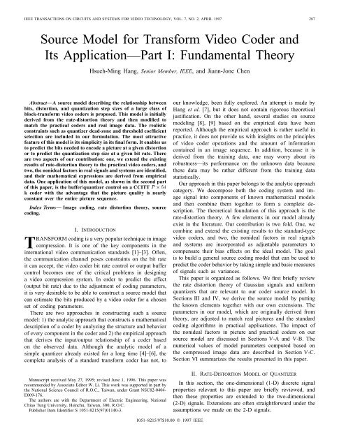
IEEE TRANSACTIONS ON CIRCUITS AND SYSTEMS FOR VIDEO TECHNOLOGY, VOL. 7, NO. 2, APRIL 1997 287
Source Model for Transform Video Coder and
Its Application—Part I: Fundamental Theory
Hsueh-Ming Hang, Senior Member, IEEE, and Jiann-Jone Chen
Abstract—A source model describing the relationship between
bits, distortion, and quantization step sizes of a large class of
block-transform video coders is proposed. This model is initially
derived from the rate-distortion theory and then modified to
match the practical coders and real image data. The realistic
constraints such as quantizer dead-zone and threshold coefficient
selection are included in our formulation. The most attractive
feature of this model is its simplicity in its final form. It enables us
to predict the bits needed to encode a picture at a given distortion
or to predict the quantization step size at a given bit rate. There
are two aspects of our contribution: one, we extend the existing
results of rate-distortion theory to the practical video coders, and
two, the nonideal factors in real signals and systems are identified,
and their mathematical expressions are derived from empirical
data. One application of this model, as shown in the second part
of this paper, is the buffer/quantizer control on a CCITT P 2 64
k coder with the advantage that the picture quality is nearly
constant over the entire picture sequence.
Index Terms— Image coding, rate distortion theory, source
coding.
I. INTRODUCTION
TRANSFORM coding is a very popular technique in image
compression. It is one of the key components in the
international video communication standards [1]–[3]. Often,
the communication channel poses constraints on the bit rate
it can accept, the video coder bit rate control or output buffer
control becomes one of the critical problems in designing
a video compression system. In order to predict the effect
(output bit rate) due to the adjustment of coding parameters,
it is very desirable to be able to construct a source model that
can estimate the bits produced by a video coder for a chosen
set of coding parameters.
There are two approaches in constructing such a source
model: 1) the analytic approach that constructs a mathematical
description of a coder by analyzing the structure and behavior
of every component in the coder and 2) the empirical approach
that derives the input/output relationship of a coder based
on the observed data. Although the analytic model of a
simple quantizer already existed for a long time [4]–[6], the
complete analysis of a standard transform coder has not, to
our knowledge, been fully explored. An attempt is made by
Hang et al. [7], but it does not contain rigorous theoretical
justification. On the other hand, several studies on source
modeling [8], [9] based on the empirical data have been
reported. Although the empirical approach is rather useful in
practice, it does not provide us with insights on the principles
of video coder operations and the amount of information
contained in an image sequence. In addition, because it is
derived from the training data, one may worry about its
robustness—its performance on the unknown data because
these data may be rather different from the training data
statistically.
Our approach in this paper belongs to the analytic approach
category. We decompose both the coding system and image
signal into components of known mathematical models
and then combine them together to form a complete description.
The theoretical foundation of this approach is the
rate-distortion theory. A few elements in our model already
exist in the literature. Our contribution is two fold. One, we
combine and extend the existing results to the standard-type
video coders, and two, the nonideal factors in real signals
and systems are incorporated as adjustable parameters to
compensate their bias effects on the ideal model. The goal
is to build a general source coding model that can be used to
predict the coder behavior by taking simple and basic measures
of signals such as variances.
This paper is organized as follows. We first briefly review
the rate distortion theory of Gaussian signals and uniform
quantizers that are relevant to our coder source model. In
Sections III and IV, we derive the source model by putting
the known elements together with our own extensions. The
parameters in our model, which are originally derived from
theory, are adjusted to match real pictures and the standard
coding algorithms in practical applications. The impact of
the nonideal factors in picture and practical coders on our
source model are discussed in Sections V-A and V-B. The
numerical values of model parameters computed based on
the compressed image data are described in Section V-C.
Section VI summarizes the results presented in this paper.
Manuscript received May 27, 1995; revised June 1, 1996. This paper was
recommended by Associate Editor W. Li. This work was supported in part by
the National Science Council of R.O.C., Taiwan, under Grant NSC82-0404-
E009-176.
The authors are with the Department of Electric Engineering, National
Chiao Tung University, Hsinchu, Taiwan, 300, R.O.C.
Publisher Item Identifier S 1051-8215(97)01140-3.
II. RATE-DISTORTION MODEL OF QUANTIZER
In this section, the one-dimensional (1-D) discrete signal
properties relevant to this paper are briefly reviewed, and
then these properties are extended to the two-dimensional
(2-D) signals. Extensions are often straightforward under the
assumptions we made on the 2-D signals.
1051–8215/97$10.00 © 1997 IEEE

288 IEEE TRANSACTIONS ON CIRCUITS AND SYSTEMS FOR VIDEO TECHNOLOGY, VOL. 7, NO. 2, APRIL 1997
Fig. 1.
Signal decomposition using transform.
A. Stationary Gaussian Process
The following results known in information theory are the
bases of our future discussions. First, if a (composite) signal
can be decomposed into two or more independent components,
then its (total) rate-distortion function can be derived directly
from the rate distortion functions of the individual components.
In theory, there is no loss of compression efficiency in
decomposing a composite signal into simpler components and
then compressing each component independently [6].
Second, the rate distortion functions of a few independent
identically distributed (i.i.d.) sources are known such as the
i.i.d. Gaussian sequence. Based on the proposition stated
in the above, the rate-distortion functions of signals with
memory can be derived by decomposing these signals into
independent components with known rate-distortion functions.
An example is the stationary Gaussian process. We can apply
Fourier transform to it and transformed frequency components
are i.i.d. Gaussian sequences. This procedure also suggests
a way for compression. That is, an optimal procedure for
compressing stationary random processes is to transform a
composite signal into independent components and then apply
the ordinary data compression techniques to each component
separately [10]. A pictorial illustration of this concept is shown
in Fig. 1.
The well-known rate distortion function of a discrete stationary
Gaussian process under the mean square distortion
criterion is given as [6], [10]
(1)
can possibly be achieved at bit rate . In (1) and (2), is a
dummy parameter whose value is decided by a selected
or value. The above formulas suggest that to achieve the
optimum coding performance, the frequency components of
power less than should be discarded and an amount of
distortion should be imposed on every one of the retained
frequency components.
In reality, we cannot use infinite length transforms to
decompose a signal sequence. A typical approach is to partition
a signal sequence into nonoverlapped blocks and perform
block transformation on each data block separately. There
are two problems associated with this approach. One is the
correlation among the neighboring blocks, which can be
significant for the low frequency components. A part of
this correlation can be reduced by applying another layer
of correlation reduction techniques on the low frequency
components of nearby blocks. The other problem is the power
spectrum used in (1) and (2). Practically, the signal power
spectrum has to be estimated from data samples. A simple
and popular spectrum estimation method is the periodogram
that computes the spectrum based on the weighted average of
the Fourier transforms of nonoverlapped data blocks [11]. This
method is consistent with the finite-size transform we use in
data compression if we view the block transform components
as the discrete approximation of the ideal continuous power
spectrum. Assuming a uniform sampling grid in the frequency
domain, (1) and (2) can thus be approximated by the following
discrete versions:
and
where is the number of samples in a data block, and
. This is exactly the system
represented by Fig. 1 with components.
One may note that (3) can be rewritten as
(3)
(4)
and
(2)
(5)
where and is the power spectrum density function
of , and
Region
and
Region .
An interpretation of the above formula is that is the
minimum bit necessary to achieve an average distortion
by an ideal coder of possibly unbounded complexity and time
delay. Similarly, is the minimum average distortion that
where . An interesting property of the above equation
is that the exponential function of bit rate is proportional to
the product of the variances of the signal components rather
than the sum of variances.
A case of interest is that at low distortion when
(or is empty), (4) becomes . And thus,
(5) becomes
(6)

HANG AND CHEN: SOURCE MODEL FOR TRANSFORM VIDEO CODER AND ITS APPLICATION—PART I 289
or
where
(7)
(8)
Essentially, we are approximating a joint Gaussian source
by multiple i.i.d. Gaussian sources. If the approximation
errors can be viewed as white noise, because the power of
high frequency components is much lower than that of low
frequency components for typical images, the SNR values
of high frequency components are smaller. According to (7)
and (8), the total distortion is proportional to the product of
component power. Hence, a 50% error in one component
would translate to 50% total error. Therefore, we should
weight the higher frequency components less in the process of
selecting quantization parameters in coding. In addition, the
unequal frequency weighting also matches the uneven human
visual sensitivity.
There are two frequency weighting approaches. One is using
the uneven frequency-dependent weights in assigning bits to
each frequency component in (3). The other is using uneven
weights in computing the total distortion in (4). A special case
of the former, frequency-weighted bit allocation, is discussed
in Section II-C. A study of the latter, the frequency-weighted
distortion case, has been described in [12]. Both approaches,
in fact, would lead to similar yet not identical results.
An interesting point of (7) is that the bits and distortion
of a (composite) signal are decided by a single parameter ,
which is the product of all the components’ variances. Thus,
we may call the entropy variance of a signal. It represents
the complexity of the signal. The signal entropy is proportional
to . In theory, two signals of the same ordinary variance
require different numbers of bits in coding if their entropy
variances are significantly different.
Assuming the 2-D signals we are dealing with are separable
in the horizontal and the vertical directions, then all the
above properties can readily be extended to the 2-D signals
without significant modifications. The Karhunen–Loève (K–L)
transform is recognized as the optimal transform for decorrelating
signals and packing the signal energy to the fewest
number of transform coefficients. However, K–L transform is
data dependent and is computationally intensive because it is
derived from the signal autocovariance function. In practical
applications, the separable discrete cosine transform (DCT) is
often adequate for most of the natural pictures and thus is
widely used [12].
B. Quantization
The lossy compression element in Fig. 1 is often, in practice,
implemented by a quantizer and an entropy coder such as
in JPEG and MPEG. Although the vector quantizer offers
potentially better compression efficiency, the scalar quantizer
is often used in real systems not only due to its simplicity but
also due to its adaptability to the local pictorial data as will
be discussed in Section IV.
Fig. 2. Entropy of uniform quantizer for sources of different probability
density functions (PDF’s).
Fig. 3.
PDF’s.
Mean square error of uniform quantizer for sources of different
A uniform midtread quantizer (in which zero is a reconstruction
level) is often used in a practical coding system.
Typically, the reconstruction levels are the centers of the
decision regions, i.e.,
, where
is the quantization step size. The behavior of such a
quantizer has been analyzed for inputs with known probability
distributions. Except for the uniform distribution, closedform
formulas of entropy, , and distortion, , for
arbitrary probability distributions are generally unavailable.
The formulation of and for uniform, Gaussian,
and Laplacian distributions are described in the Appendix. The
numerical values of these functions are plotted in Figs. 2 and
3. The “Reference” curves in Figs. 2 and 3 are computed using
(9) and (10) with (see below).
It is known that, at high bit rates (small distortion), the
bits ( ) versus distortion ( ) relation of an entropy-coded
uniform quantizer for a zero-mean i.i.d. source can be

290 IEEE TRANSACTIONS ON CIRCUITS AND SYSTEMS FOR VIDEO TECHNOLOGY, VOL. 7, NO. 2, APRIL 1997
Fig. 4.
Practical image transform coder.
approximated by the following formulas [4], [12]:
and
Thus
(9)
(10)
(11)
where is 12 and is 1.386 ( ) for uniform,
Gaussian, and Laplacian distributions, is source dependent
and is about one for uniform distribution, 1.4 for Gaussian,
and 1.2 for Laplacian, and is the signal variance. As
shown by Figs. 2 and 3, the above approximations are fairly
accurate when the quantization step size is smaller than the
signal standard deviation. Combining (9) and (10) we obtain
(12)
This gives us a more direct relation between and .
In image coding, bits are typically spent on a small percentage
of dominant transform coefficients of which the allocated
bit rates are often higher than a couple of bits per coefficient.
Although there is no simple and accurate formula for the low
variance coefficients, these coefficients do not affect the overall
model very much since their contribution in bits is relatively
small. Therefore, the above formulas, although are accurate
for medium to high bit rates, they are still practically useful
for all the bit rates of interest.
In a real system, the ideal entropy coder is typically replaced
by a variable-length coder (VLC), a simplified version of
Huffman code [13]. Assuming this VLC is nearly as efficient
as the ideal entropy coder, the bits produced by this VLC, ,
may be approximated by , where is the ideal entropy
bits of the quantizer outputs, and is a scaling factor (for
adjustment) greater than one. Under this assumption, (12) may
still be used for a practical scalar quantizer with a modified
value of (to be discussed in Section V).
III. PRACTICAL TRANSFORM CODER
A practical image transform coder, such as the DCT coders
used in [1]–[3], can be represented by the general block
diagram in Fig. 4. It follows roughly the aforementioned
principles, namely, a transform (DCT) used to decompose
the original pictures into nearly independent components, a
uniform scalar quantizer used to reduce the output levels, and
a VLC used to further compress the output bit stream. As
compared to that described in Sections II-A and II-B, the individual
entropy coders are replaced by a data model followed
by an entropy coder. The objective of transformation and data
model together is to produce (nearly) statistically independent
data sequences so that they can be coded separately with high
efficiency.
The data model used in [1]–[3] simply rearranges the
transform coefficients in a zigzag scan order. That is, the
2-D array of a block of DCT coefficients are assembled
to form a zigzag scanned 1-D linear array or vector
, in which the lower frequency’s DCT coefficients
are usually associated with smaller indices. When
the coefficients are ordered in this fashion, the variances of
coefficients are approximately monotonically decreasing [2].
If the transformed source vector
is
stationary and every frequency component is independent, then
the average entropy per block,
, equals the
sum of the entropies of all the components.
According to [12] and [14], the conditions discussed in
the above, to a great extent, satisfied; that is, the frequency
components (transform coefficients) are nearly i.i.d. sources,
the distortion of quantized coefficients are relatively small,
and the VLC performance is close to that of the ideal entropy
coder. Then, the behavior of such a transform coder can be
derived from (9) or (11) by combining all the components
together. Assuming the probability distribution of the frequency
components is either uniform, Gaussian, or Laplacian,
and is the average bits of the th entropy-coded, quantized
coefficient, the total average bits of such a source is
(13)
(14)
where , , and are the distortion, the variance, and
the parameter associated with the th component. Since
(10)
(15)

HANG AND CHEN: SOURCE MODEL FOR TRANSFORM VIDEO CODER AND ITS APPLICATION—PART I 291
where is the quantization step size of the th component,
and is the parameter associated with that component.
Due to the frequency-dependent visual sensitivity of human
perception [12], bits assigned to a frequency component should
be adjusted according to their perceptual threshold. Thus,
the quantization step size of each transform coefficient, ,
can be different in JPEG [2] and MPEG
[3]. In addition, the quantization step sizes in MPEG are made
of two components: , a quantization scaling factor for the
entire picture block, and
, a weighting
matrix whose elements are used as multiplicative factors to
produce the true step sizes in quantization. In other words,
. On the other hand, the H.261 specification
assumes that all the step sizes in a block are identical [1], that
is, for all . The frequency-dependent step size design
implies a frequency-weighted bit allocation scheme discussed
in Section II-A in the sense that some frequency components
get assigned fewer bits because their actual step sizes used in
quantization are larger; that is [from (12)]
with
and
Therefore, (14) and (15) become
(16)
(17)
(18)
They completely describe the bits and distortion behavior of an
MPEG or JPEG transform coder under the ergodic Gaussian
signal assumption. A special case that and for
all has been reported in [7].
In reality, a frequency component may have an effective
variance
less than the weighted distortion,
. Also, as the theory predicts, the value of is close
to 12 when is much higher than , but its value may
be different if is close to or smaller than . We then
need to go back to (3) and (4), and modify (17) and (18) to
the following:
where regions of and are
and
(19)
(20)
is the size of set
, and
Using optimization techniques, Netravali and Haskell derived
similar but not identical results under the frequency-weighted
distortion criterion [12].
IV. THRESHOLD TRANSFORM CODER
In digital image coding, theory and practice do not agree
completely due to several nonideal factors. First, the assumptions
undertaken by theory (in the previous sections) such as
ergodicity and stationary of image sources do not hold exactly
on real data. Second and more importantly, the human visual
system is highly nonlinear and cannot be approximated by
a simple distortion measure such as the mean square error
(MSE). For example, a very small percentage of a coded
picture bearing visible artifacts does not affect the overall MSE
very much; however, a human viewer can easily pick up the
distorted areas, and thus the entire picture quality is rated low.
Therefore, in image coding we have to deal with not only the
statistical behavior of the entire picture (objective criterion)
but also the fidelity of individual samples embedded in their
texture neighborhood (subjective criterion).
Several intuitive schemes have been proposed to solve
the above problem. Instead of selecting a fixed number of
transform coefficients according to their average variances
as suggested by the theory, we select the coded coefficients
by their magnitudes, the so-called threshold transform coding.
The direct implementation of threshold coding requires
transmitting the threshold mask—locations of the chosen coefficients—which
often needs a significant number of bits. A
popular approach is rearranging the transform coefficients in
a fixed scanning order, transmitting them sequentially until
the last above-threshold coefficient is hit, and then appending
an end-of-block code to conclude this data block. The exact
analysis of such a coder is involved and may not be worth
the efforts since the real image data do not match exactly
our stationary model assumption. The following simplification
seems to be sufficient for image coding purpose.
Our focus is on the bit-distortion model, i.e., the average bits
and distortion associated with a typical block. Assuming that
is the threshold value used in picking up the th transform
coefficient; that is, the th coefficient is set to zero before
quantizing if its magnitude is less than . A popular variant of
this scheme is the dead zone quantizer—the decision region of
the zero reconstruction level is larger than the decision region
used for the other reconstruction levels. In both cases and the
combined situation, the analysis of such quantizers is similar
to that of a simple uniform quantizer; however, the decision
levels and the reconstruction levels have to be modified in
the analysis equations. Details of the above modifications are
described in the Appendix.
For various threshold ( ) values, the entropy versus distortion
curves of a uniform quantizer with a dead zone set
to
are plotted in Figs. 5 and 6. The

292 IEEE TRANSACTIONS ON CIRCUITS AND SYSTEMS FOR VIDEO TECHNOLOGY, VOL. 7, NO. 2, APRIL 1997
(a)
(a)
(b)
(b)
(c)
Fig. 5. Entropy of quantizers with dead-zone for (a) uniform, (b) Gaussian,
and (c) Laplacian sources.
(c)
Fig. 6. MSE of quantizers with dead-zone for (a) uniform, (b) Gaussian,
and (c) Laplacian sources.

HANG AND CHEN: SOURCE MODEL FOR TRANSFORM VIDEO CODER AND ITS APPLICATION—PART I 293
Reference curves shown on those plots are the asymptotic
formulas described by (9) and (10).
In image coding, the quantization step sizes of significant
frequency components are usually smaller than the signal
standard deviation; therefore, (10) and (12) are reasonably
good approximations if , , and are adjusted appropriately.
The values of these parameters, in general, depend upon and
. However, for a fixed and a certain range of step sizes,
they can be approximated by constants. When the step size
gets larger, (10) and (12) become less accurate. But in these
cases the bits produced by those coefficients are very small and
thus do not change very much the total bits. Extensions and
modifications of these parameters are described in the next
section.
Assuming that the bits on the average needed to encode
an above-threshold transform coefficient are represented by
[from (12)]
(21)
these curves and have about the same value for all the three
distributions. Therefore, replacing in (23) by ,we
obtain
where
(25)
where , is the threshold value used in picking up
the th transform coefficient, and and are sourcedependent
parameters. The average bits number of a pixel
becomes
Or
(26)
(27)
(22)
where are the bits for the end-of-block signal.
If the weighting matrix in (17) is adopted, the average bits
and the average distortion can be made more explicit
and
(23)
(24)
Since the threshold transform coding with weighting matrix
is invented to match the subjective distortion criterion, the
mean square error distortion calculation, (24), is not as useful
as the bits calculation, (23), which can be used to adjust the
quantization step for regulating encoder buffer and controlling
picture quality.
If is chosen to be with roughly
the same constant value for all the coefficients, then , ,
and can be expressed as functions of and only.
Also, in most image coding cases, the ac components have
approximately Laplacian distribution and the dc component,
uniform or Gaussian distribution [12]. Hence, the values
are similar for all the frequency components as indicated
by Fig. 5, in which ’s are proportional to the slopes of
with . Note that we denote by
in the above equations for simplicity.
The direct use of (25) seems to be fairly complicated—it
needs to estimate a number of parameters, ’s, ’s,
and , computed from image data. If, however, we could
assume that the picture to be coded is not much different from
the picture that has already been coded in the sense that the
, and remain about the same in the neighborhood of
that we are dealing with, then the parameter in (27) can
be estimated from the and of the coded pictures. Typically,
the value is less picture-dependent, only the value has to
be estimated from image data. Consequently, the entire model
identification procedure can be relatively simple.
V. MODEL PARAMETERS
For a practical application, the parameters of the above
model have to be adjusted to cope with the specific video coder
used and the real picture characteristics. The meaning of the
parameters in our model (23) and (24) suggests the following
modifications. First, since is a factor mainly determined
by probability distribution, we assume is a constant ( 1.2
for Laplacian source, say) for the rest of analysis. Second,
the value of is no longer constant for small ;
however, those values can be precalculated and stored in a
table for real-time applications. Third, the constant
is replaced by a parametric function
to compensate for the mismatch between the ideal model and
a practical video coder. Although these parameters ( , , and
) may be somewhat related, for simplicity we study them
separately. We will elaborate on the second and the third items
below.

294 IEEE TRANSACTIONS ON CIRCUITS AND SYSTEMS FOR VIDEO TECHNOLOGY, VOL. 7, NO. 2, APRIL 1997
A. Model Parameter
We wish to find the model parameter for different and
under the assumption that is a constant ( 1.2). If
the quantization error is i.i.d. and is uniformly distributed,
the theoretical value of is 12. This is approximately true
when the quantization step is much smaller than the signal
variance (the left portion of Fig. 7). However, the above
assumption is not valid for large quantization step sizes.
Since the high frequency transform coefficients are roughly
Laplacian distributed, we are interested in the Laplacian cases.
Combining (21) and (A9) in the Appendix, we obtain the
value for the Laplacian probability distribution
(28)
The values calculated based on this formula are plotted in
Fig. 7. From Fig. 7, we find that increases abruptly after
exceeds a threshold value ( 1.3). This is because
when the quantization step size is very large (comparing to
the signal variance), quantization errors can no longer be
treated as uniformly distributed. Therefore, the distortion goes
up at a slower pace than the asymptotic formula predicts.
Eventually, the distortion saturates when it approaches the
signal variance (Fig. 6). However, in order to use the same
distortion function, (10), for the cases that their distortion is
approaching signal variance, the corresponding values are
made growing exponentially (Fig. 7). In real-time applications,
it is not likely to compute
directly based upon
the above equations. For a specific system, MPEG say, we
choose a fixed ( in this instance) and build
a look-up table for real-time use. We did the same thing in
the following simulations. One may note from Fig. 5(c) that
entropy 0 when . Hence the look-up table
needs only to store the values for smaller than
1.5. For 1.5, the corresponding distortion value
is , and in this case, based on the original definition of in
(10), becomes . On the other extreme for
, a constant of 12 is assigned to .
B. Nonideal Factors in a Practical Coder and Parameter
Mismatches between the theoretical entropy model and the
real VLC coded bits are discussed in this section. Several scaling
factors are observed and estimated from experimental data
to compensate for the mismatches. In Section II, is initially
treated as constant ( 1.386), but later analysis suggests that
varies depending upon the value of quantization step size.
First, the probability density functions (PDF’s) of the ac
coefficients are not ideal Laplacian distribution of equal variance.
This PDF mismatch, shown in Fig. 8, results in a smaller
entropy for real transform coefficients than the predicted value
based on Laplacian assumption. As the quantization step
increases, the probability of the quantized values around zero
grows much larger than that of the other intervals, and the
PDF mismatch problem becomes even more serious. We thus
introduce a multiplicative factor to compensate for the
difference. Second, the transform coefficients within a block
Fig. 7. Model parameter for various dead-zone values (T ) and quantization
step sizes (delta).
are somewhat correlated; hence, another multiplicative factor,
, is introduced to correct the original i.i.d. assumption.
Third, the VLC table in image coding standards is built based
on the probability of zero coefficient runs and coefficient
levels, (run, level), rather than on .
Therefore, the average encoded bits per block are higher than
the theoretical block entropy. We denote this inefficiency of
VLC table by the third multiplicative parameter .
Combining these factors together as a whole, we obtain
bits
bits (29)
where bits represents the real coded bits. All the above
multiplicative scaling factors are functions of quantization
scale ( ). Hence, the overall factor is, in general, a function
of . Practically, we only need to estimate the overall factor
from the real data. Therefore, (27) is still valid when
is replaced by bits , as long as the new includes
the nonideal factor .
In summary, the original [ in (25) and (27)] is now
replaced by , where is a function of ,
and it includes the nonideal factors in entropy coding. Once we
decide the value (Section V-A), (27) can be used to compute
from data. An H.261-type coding structure is used as
an example. Since the dc coefficients are coded with fixed
length codewords and their coding is independent of the ac
coefficients coding, we concentrated on the statistical analysis
of the ac coefficients. Fig. 9 shows the values computed
from the intracoded frames of several video sequences at
different values. In this experiment, the values are taken
from Fig. 7, is set to “1” for all the frequency components,
and is neglected.

HANG AND CHEN: SOURCE MODEL FOR TRANSFORM VIDEO CODER AND ITS APPLICATION—PART I 295
(a)
Fig. 9.
Model parameter s(qs) for various pictures.
and
.
Thus far, we have obtained the parametric formulas of
and . These expressions can be used
to estimate the bits needed to encode a picture with a prechosen
quantization scale.
(b)
Fig. 8. Probability density functions (solid line) of the first ac component
of transform coefficients for (a) Salesman and (b) Claire. The dash lines are
Laplacian density functions of the same variance, and the dotted lines are
Gaussian density functions of the same variance.
It can be seen that the values are getting larger
and approaching one when the quantization scales are getting
small. This is because the quantized coefficients are less
correlated at small quantization scales. Hence, the encoded
bits are well estimated by our original entropy model. For
larger quantization step sizes, the original model predicts fewer
bits than the true bits. To compensate for this fact, is
significantly smaller than one for large .
In order to use our model in predicting coded bits, we look
for a simple arithmetic expression of . A first-order linear
curve fitting is obtained from experimental data as follows:
(30)
where and are two picture dependent constants. Since
is an indication of image complexity,
we derive the following empirical formulas for typical values
of and
C. Bits Prediction
If the coded bits can be predicted prior to the quantization
and VLC operations, then the coding process can be well
controlled. Based on (25), (27), and the parameters and
described in the preceding subsection, bits needed to
encode a picture for a given distortion (quantization step)
can be estimated if the variances of transform coefficients
are available. The picture characteristics from coding point of
view are completely specified by the function in (27).
This function, , can thus be considered as the measure
of picture coding complexity and therefore is named “coding
complexity function.” If we keep in (27) as a constant
and allow to vary to accommodate for the varying
, the computation in quantizer control procedure can
then be simplified somewhat. In this case, the resultant
is called “modified ” and is denoted by . For
easy distinction, we call the “original ” denoted
by if it is computed using (27) directly based on
the variances of block transform coefficients. Some examples
of and are shown in Fig. 10. An interesting
observation is that both and can be approximated
rather well by a linear equation (for each picture separately)
when ’s are relatively small (between 10 and 30), which are
the most frequently used values in practice. In other words
(31)
where and are two picture-dependent constants. We
can see from Fig. 10(a) and (b) that the coded bits of different
pictures are reflected on their corresponding coding complexity
functions. If the picture contents do not change significantly

296 IEEE TRANSACTIONS ON CIRCUITS AND SYSTEMS FOR VIDEO TECHNOLOGY, VOL. 7, NO. 2, APRIL 1997
(a)
step sizes for block-transform coders. This source model is
initially derived based on rate-distortion theory. The realistic
constraints such as quantizer dead-zone and threshold coefficient
selection are included in our formulation. The picture
complexity from a coding point of view can be measured
and computed from the entropy variance which is the product
of all the component’s variances of image signals. When the
model is used in real video coding, image characteristics and
nonideal factors of a practical video coder are accommodated
by parameterizing the model constants. If the parameter values
are properly chosen, the coding behavior can be well estimated
by the proposed model. In brief, there are two aspects of
our contribution. One, we extend the existing results of ratedistortion
theory to the practical video coders, and two, the
nonideal factors in real signals and systems are identified and
their mathematical expressions are derived from experimental
data. One application of this source model, as shown in the
second part of this paper, is the buffer/quantizer control in
video coders with the advantage that the picture quality is
kept nearly constant over the entire picture sequence.
APPENDIX
ENTROPY AND DISTORTION OF UNIFORMLY
QUANTIZED UNIFORM AND LAPLACIAN SOURCES
A. Uniform Quantizer
The behavior of a uniform quantizer can be analyzed by
the following equations for inputs with known probability
distributions. Assuming that the probability density function of
a zero-mean i.i.d. source is , the entropy bits produced
by this uniform quantizer can be calculated by
(A1)
(b)
Fig. 10. The coding complexity function for various pictures (the first
frame in those picture sequences). (a) Coded bits per pixel for various
quantization step sizes and (b) the modified F (q s )(F m (qs)) and the original
F (qs)(F o (qs)) values.
between two nearby frames, the computed from the
previous frame can still be used to estimate the bits of the
current frame at similar step sizes.
We should keep in mind that the above bits model is derived
based on several assumptions of the statistical behavior of
data. For real pictures and picture sequences, the stationarity
and ergodicity assumptions are not completely satisfied. In
addition, this simple model uses essentially only to
estimate the bits needed to encode an entire picture. Although
is made a function of , it is not possible to cover all
the nonstationarity and data-dependency fully by only a couple
of parameters. Therefore, a small amount of estimation errors
cannot be avoided.
VI. CONCLUSIONS
In this paper, we derive a source model that describes
the relationship between bits, distortion, and quantization
where
and the mean square quantization error is
(A2)
(A3)
where decides the total number of quantization levels
( ), chosen sufficiently large to eliminate almost all the
overloaded quantization errors.
B. Uniform Distribution
Assuming that a zero-mean uniform distribution i.i.d. source
with variance is quantized by a uniform quantizer described
above. Then, the entropy of the outputs is [5]
(A4)

HANG AND CHEN: SOURCE MODEL FOR TRANSFORM VIDEO CODER AND ITS APPLICATION—PART I 297
and the mean square quantization error is
(A5)
For Laplacian distribution, let
.
The entropy (in bits) and distortion can be derived
, and
C. Gaussian Distribution
The probability density function of a zero-mean Gaussian
source with variance is
Unfortunately, there are no closed form formulas of (A1) and
(A3) for Gaussian distribution. However, in this case, it is not
difficult to compute their numerical values using (A1) and
(A3). The results are shown in Figs. 5(b) and 6(b). When
is reasonably small, the PDF is approximately
constant in a -width interval. We then obtain the asymptotical
behavior of such a quantizer at high bit rates as indicated by
(9) and (10).
D. Laplacian Distribution
The probability density function of a zero-mean Laplacian
source with variance is
and
If we take the centroid of the decision region
the reconstruction level, we obtain
(A9)
(A10)
as
(A11)
Thus
A uniform quantizer without dead zone may be considered
as a special case of the above with . In this case, the
corresponding entropy and distortion are
(A6)
The general formulas of entropy and distortion of uniformlyquantized
Laplacian source with dead-zone are given below.
E. Dead Zone
Assume that the first reconstruction level of a quantizer with
dead-zone is , then the reconstruction levels are
and
where
(A12)
(A13)
(A14)
If the corresponding input decision regions are selected as
F. Threshold
If a dead-zone quantizer also has a threshold
, then (A7) and (A8) are modified to
and
then (A2) and (A3) are modified to
and
(A7)
(A15)
(A8)
otherwise

298 IEEE TRANSACTIONS ON CIRCUITS AND SYSTEMS FOR VIDEO TECHNOLOGY, VOL. 7, NO. 2, APRIL 1997
and
[9] W.-Y. Sun, H.-M. Hang, and C. B. Fong, “Scene adaptive parameters
selection for MPEG syntax based HDTV coding,” in Signal Processing
of HDTV, L. Stenger et al., Eds. Elsevier Science, 1994, vol. V.
[10] A. J. Viterbi and J. K. Omura, Principles of Digital Communications
and Coding. New York, NY: McGraw-Hill, 1979.
[11] A. V. Oppenheim and R. W. Schafer, Discrete-Time Signal Processing.
Englewood Cliffs, NJ: Prentice Hall, 1989.
[12] A. N. Netravali and B. G. Haskell, Digital Pictures: Representation and
Compression. New York, NY: Plenum, 1988.
[13] R. E. Blahut, Principles and Practice of Information Theory. Reading,
MA: Addison-Wesley, 1991.
[14] K. R. Rao and P. Yip, Discrete Cosine Transform: Algorithms, Advantages,
Applications. San Diego, CA: Academic, 1990.
where
(A16)
and represents the smallest integer that is greater than or
equal to . When , the threshold operation
is not effective. It then simply becomes a regular uniform
quantizer.
REFERENCES
[1] CCITT, Working Party XV/1, “Draft of recommendation H.261: video
codec for audiovisual services at P 2 64k bits/s,” July 1990.
[2] W. B. Pennebaker and J. L. Mitchell, JPEG—Still Image Data Compression
Standard. New York, NY: Van Nostrand Reinhold, 1993.
[3] MPEG (Motion Picture Experts Group, ISO–IEC JTC1/SC29/WG11),
“Coding of Moving Pictures and Associated Audio,” CD 11172-2 Nov.
1991.
[4] H. Gish and J. N. Pierce, “Asymptotically efficient quantizing,” IEEE
Trans. Inform. Theory, vol. IT-14, pp. 676–683, Sept. 1968.
[5] N. S. Jayant and P. Noll, Digital Coding of Waveforms. Englewood
Cliffs, NJ: Prentice Hall, 1984.
[6] T. Berger, Rate Distortion Theory. Englewood Cliffs, NJ: Prentice
Hall, 1971.
[7] H.-M. Hang et al., “Digital HDTV compression using parallel motioncompensated
transform coders,” IEEE Trans. Circuits Syst. Video Technol.,
vol. 1, pp. 210–221, June 1991.
[8] A. Puri and R. Aravind, “Motion-compensated video coding with
adaptive perceptual quantization,” IEEE Trans. Circuits Syst. Video
Technol., vol. 1, pp. 351–361, Dec. 1991.
Hsueh-Ming Hang (S’79–M’84–SM’91) received
the B.S. and M.S. degrees from National Chiao
Tung University, Hsinchu, Taiwan, in 1978 and
1980, respectively, and the Ph.D. in electrical engineering
from Rensselaer Polytechnic Institute, Troy,
NY, in 1984.
From 1984 to 1991, he was with AT&T Bell
Laboratories, Holmdel, NJ, where he was engaged
in digital image compression algorithm and architecture
researches. He joined the Electronics Engineering
Department of National Chiao Tung University,
Hsinchu, Taiwan, in December 1991. His current research interests include
digital video compression, image/signal processing algorithm and architecture,
and digital communication theory.
Dr. Hang was a conference co-chair of Symposium on Visual Communications
and Image Processing (VCIP), 1993, and the Program Chair of
the same conference in 1995. He guest co-edited two Optical Engineering
special issues on visual communications and image processing in July 1991
and July 1993. He was an Associate Editor of IEEE TRANSACTIONS ON IMAGE
PROCESSING from 1992 to 1994 and a Co-Editor of the book Handbook of
Visual Communications (Academic Press, 1995). He is currently an Editor of
Journal of Visual Communication and Image Representation, Academic Press.
He is a member of Sigma Xi.
Jiann-Jone Chen was born in Tai-Chong, Taiwan,
R.O.C., in 1966. He received the B.S. and
M.S. degrees in electrical engineering from National
Cheng Kung University, Tainan, in 1989 and 1991,
respectively. He is currently working toward the
Ph.D. degree in electronics engineering at National
Chiao Tung University, Hsinchu, Taiwan.
His research interests include medical image processing
and digital video coding.