Pragmatic, Unifying Algorithm Gives Power Probabilities for ...

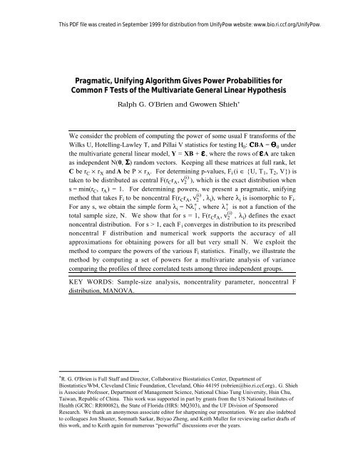
This PDF file was created in September 1999 for distribution from UnifyPow website: www.bio.ri.ccf.org/UnifyPow. 

Pragmatic, Unifying Algorithm Gives Power Probabilities for 

Common F Tests of the Multivariate General Linear Hypothesis 

Ralph G. O'Brien and Gwowen Shieh * 

We consider the problem of computing the power of some usual F transforms of the 

Wilks U, Hotelling-Lawley T, and Pillai V statistics for testing H 0 : CBA = Œ 0 under 

the multivariate general linear model, Y = XB + ‰, where the rows of ‰A are taken 

as independent N(0, Í) random vectors. Keeping all these matrices at full rank, let 

C be r C × r X and A be P × r A . For determining p-values, F i (i ∈ {U, T 1 , T 2 , V}) is 

taken to be distributed as central F(r C r A , ν (i) 

2 ), which is the exact distribution when 

s = min(r C , r A ) = 1. For determining powers, we present a pragmatic, unifying 

method that takes F i to be noncentral F(r C r A , ν (i) 

2 , λ i ), where λ i is isomorphic to F i . 

For any s, we obtain the simple form λ i = Nλ ∗ i , where λ ∗ i is not a function of the 

total sample size, N. We show that for s = 1, F(r C r A , ν (i) 

2 , λ i ) defines the exact 

noncentral distribution. For s > 1, each F i converges in distribution to its prescribed 

noncentral F distribution and numerical work supports the accuracy of all 

approximations for obtaining powers for all but very small N. We exploit the 

method to compare the powers of the various F i statistics. Finally, we illustrate the 

method by computing a set of powers for a multivariate analysis of variance 

comparing the profiles of three correlated tests among three independent groups. 

KEY WORDS: Sample-size analysis, noncentrality parameter, noncentral F 

distribution, MANOVA. 

* R. G. O'Brien is Full Staff and Director, Collaborative Biostatistics Center, Department of 

Biostatistics/Wb4, Cleveland Clinic Foundation, Cleveland, Ohio 44195 (robrien@bio.ri.ccf.org).. G. Shieh 

is Associate Professor, Department of Management Science, National Chiao Tung University, Hsin Chu, 

Taiwan, Republic of China. This work was supported in part by grants from the US National Institutes of 

Health (GCRC: RR00082), the State of Florida (HRS: MQ303), and the UF Division of Sponsored 

Research. We thank an anonymous associate editor for sharpening our presentation. We are also indebted 

to colleagues Jon Shuster, Somnath Sarkar, Beiyao Zheng, and Keith Muller for reviewing earlier drafts of 

this work, and to Keith again for numerous “powerful” discussions over the years.

O'Brien and Shieh: Power for the Multivariate Linear Hypothesis 

1. INTRODUCTION 

Hypothesis-driven research proposals now typically include power analyses to 

support the chosen design and sample size. Doing so promotes an early fusion of the 

study's research questions, its proposed design, the specific measures to be collected, and 

the prescribed data analyses. Of course, the power analyses should be congruent with the 

stated hypotheses and their prescribed tests. It is our experience, however, that power 

analyses for multivariate hypotheses often use only oversimplified, univariate surrogates. 

For example, a proposed multivariate analysis of variance of a factorial design might be 

supported only by a power analysis based on some univariate, two-group t tests of the 

individual measures. Such incongruence weakens the statistical plan and hurts the quality 

of the entire proposal. 

Herein we propose and assess a pragmatic strategy for computing the powers of 

specific Normal-theory hypothesis tests under the multivariate general linear model. 

Section 2 briefly reviews the noncentrality for the univariate general linear model and 

then extends it to specify approximate (sometimes exact) noncentral distributions for the 

common F transforms of the Wilks, the Hotelling-Lawley, and the Pillai statistics. Our 

method is a modification of and is asymptotically equivalent to the Muller-Peterson 

(1984) algorithm discussed in Muller, LaVange, Ramey, and Ramey (1992). But unlike 

their method, ours provides the exact noncentral F distribution whenever the hypothesis 

involves at most s = 1 positive eigenvalue of E –1 H. For s > 1, both methods designate 

approximate noncentral F distributions that converge (N → ∞) well to their limiting 

forms. But as the Monte Carlo work in Section 3 illustrates, our method is almost always 

more accurate than the Muller-Peterson, and it is sufficiently accurate for performing 

power analyses. In Section 4 we use the method to characterize how the relative powers 

of the F statistics are dependent on the structure of the s eigenvalues of the population 

version of E –1 H. Section 5 focuses on the common q-group, P-variate problem, and 

outlines an example. 

2


2. NONCENTRALITIES 

Consider the standard (fixed-effects), full-rank multivariate general linear model, Y 

= XB + ‰, where Y is N × P of rank P; X is N × r X of rank r X ; and B contains fixed 

coefficients. The rows of ‰ are taken to be independent P-variate Normal random vectors 

with mean 0 and P × P positive-definite covariance matrix Í. The usual estimates are 

Bˆ = (X′X) –1 X′Y, and Íˆ = (Y – XBˆ )′(Y – XBˆ )/(N – r X ). The multivariate general linear 

hypothesis is H 0 : CBA = Œ 0 , where C is r C × r X with full row rank, and A is P × r A with 

full column rank; thus r A ≤ P. Œ 0 is usually chosen to be 0. H 0 has ν 1 = r C r A degrees of 

freedom. 

2.1 r A = 1 

If r A = 1 so that A ≡ a, the problem simplifies to a univariate one with y ≡ Ya = 

XBa + ‰a = X∫ + ‰. The resulting estimates are ∫ˆ = Bˆ a and σˆ 2 = a′Íˆ a/(N – r X ) . H 0 

is tested with F = (SSH/r C )/σˆ 2 , where 

SSH = (C∫ˆ – Œ 0 )′[C(X′X) -1 C′] -1 (C∫ˆ – Œ 0 ) 

is the sums of squares for the hypothesis. It is well-known that F is distributed as an 

F(ν 1 , ν 2 , λ) random variable with ν 1 = r C and ν 2 = N – r X degrees of freedom and 

noncentrality 

λ = (C∫ – Œ 0 )′[C(X′X) -1 C′] -1 (C∫ – Œ 0 )/σ 2 . 

It is helpful to see (X′X) -1 decomposed into more distinct components. Letting 1 be 

the N × 1 vector of ones, then x – = N -1 X′1 is the r X -element mean vector and S X = 

N –1 (X – 1x – ′)′(X – 1x – ′) is the corresponding r X × r X covariance matrix. Then X′X = 

N(S X + x –– x ′ ) = NÁ, showing that with respect to X′X, the size of the design (N) is 

unrelated to Á, which is only dependent on the means, variances, and correlations of the 

Xs. Thus, [C(X′X) -1 C′] -1 = N[CÁ -1 C′] -1 , so 

λ = Nλ ∗ = N{(C∫ – Œ 0 )′[CÁ -1 C′] -1 (C∫ – Œ 0 )/σ 2 }. (2.1) 

3


2.2 General Strategy for r A > 1 

For r A > 1, SSH generalizes to the r A × r A sums of squares and cross products matrix 

for the hypothesis, 

H = N(CBˆ A – Œ 0 )′[CÁ -1 C′] -1 (CBˆ A – Œ 0 ). 

σˆ 2 generalizes to A′Íˆ A = E/(N – r X ), where E = A′(Y – XBˆ )′(Y – XBˆ )A. H and E are 

independent Wishart matrices, both based on A′Í A, and having r C and N – r X degrees of 

freedom, respectively. (SSH/r C )/σˆ 2 generalizes to {(N – r X )/r C }E -1 H, but by tradition 

we work with E -1 H. 

There is no generally optimal way to map E -1 H to a univariate test statistic. The 

most common ones are the Wilks Likelihood Ratio (U), Hotelling-Lawley Trace (T), and 

Pillai Trace (V) statistics, which are reviewed below. All are based on the s = min(r C , r A ) 

positive eigenvalues of E -1 H, denoted ƒ = {φ 1 , ..., φ s }, and ordered φ 1 > φ 2 > … > φ s > 0. 

U, T, and V are summarized and compared by Seber (1984), Anderson (1984), and 

numerous other books and articles, and their critical values have been widely tabled and 

charted (e.g., Seber, pp. 562-564). But in practice we usually obtain p values by 

transforming them to F-type statistics, denoted here as F i , i ∈ {U, T 1 , T 2 , V}. If r C = 1, 

each F i becomes F = (N – r X – r A + 1)φ 1 /r A , which is also an exact F random variable, as 

discussed below. For s > 1, the F i statistics are distinct, having different ν 2 (i) and λ i . 

We do not propose or study power approximations for Roy's test. For s > 1, no 

acceptable method has been developed for transforming φ 1 to an F or χ 2 statistic. No 

straightforward method exists for computing powers for Roy's statistic itself (Anderson, 

1984, pp. 332), although various approximations have been developed, as reviewed by 

Krishnaiah (1978). Roy's statistic is fundamentally different from U, T, and V, thus its 

power is not accurately discerned from the power probabilities computed for F U , F T1 

, F T2 

and F V . 

E –1 H = (E/N) –1 (H/N) = (A′SA) –1 (H/N), where S is the maximum likelihood 

estimate of Í. Whereas E is a central Wishart, H is possibly noncentral with 

noncentrality matrix 

4


Î = Ν(A′ÍA) –1 (CBA – Œ 0 )′[CÁ -1 C′] -1 (CBA – Œ 0 )} 

= N(A′ÍA) –1 H ∗ = NÎ ∗ .(2.2) 

H ∗ is the population counterpart of H/N. Let ƒ ∗ = {φ1 ∗ , ..., φ∗ 2 } to be the eigenvalues of 

Î ∗ = (A′ÍA) –1 H ∗ , the population counterpart of E –1 H. As N → ∞, Bˆ 

→ p B, 

H/N → p H ∗ , and E/N → p A′ÍA, so that NE -1 → p (A′ÍA) –1 . Thus, E -1 H → p (A′ÍA) –1 H ∗ 

and ƒ → p ƒ ∗ . 

We shall specify and asymptotically justify all F distributions using a common 

notation and logic. First, take F i to be an F random variable with ν 1 = r C r A and ν 2 

(i) 

degrees of freedom and noncentrality λ i = Nλ ∗ i , a form motivated by (2.1) and (2.2). 

Accordingly, E(F i /N) = N -1 (1 + λ i /ν 1 )[ν (i) 

2 /(ν (i) 

2 – 2)] → λ ∗ i /ν 1 , as N → ∞. Also, for 

each F i , F i /N → p f ∗ i , a constant. This leads to the approximation λ ∗ i = ν 1 f ∗ i . Each f ∗ i is a 

function of r C , r A and ƒ ∗ as specified below. Finally, we cite specific theory reviewed by 

Anderson (1984, Section 8.6.5) to outline why for the Hotelling and Pillai statistics, ν 1 F i 

converges to noncentral χ 2 distributions with the noncentralities proposed here. Likewise, 

the work of Kulp and Nagarsenker (1984) supports the convergence of ν 1 F U for the 

noncentral Wilks statistic. 

Motivated because E/(N – r X ) is the unbiased estimator of A′ÍA, Muller and 

Peterson (1984) proposed extracting the eigenvalues, ƒ (M) , of [(A′ÍA) –1 /(N – r X )][NH ∗ ]. 

Thus, ƒ (M) =[N/(N – r X )]ƒ ∗ . Furthermore, they proposed making λ (M) 

i = ν 2 (i) ν 1 f (M) i , 

where f (M) i uses ƒ (M) just as f ∗ i uses ƒ ∗ . One can easily show that for r A = 1 both 

methods lead to the exact univariate noncentrality given above. If r A > 1, λ (M) 

i < λ i , but 

λ i /λ (M) 

i → 1 as N → ∞. 

Muller and Barton (1989) used a similar strategy to define approximations of the 

non-null distributions of F statistics for univariate approaches for repeated measures 

analysis. O'Brien (1986) also applied the strategy to characterize the non-null 

distribution of the likelihood-ratio χ 2 statistic commonly used in log-linear models; c.f. 

Agresti (1990, Section 7.6.4). 

5


2.3 r A > 1 but r C = 1 (s = 1) 

It is well known that when r C = 1, the U, T, and V statistics convert identically to F 

= (N – r X – r A + 1)φ 1 /r A , which has r A and (N – r X – r A + 1) degrees of freedom. Our 

strategy gives λ = Nφ1 ∗ , where 

φ1 ∗ = (CBA – Œ 0 )(A′ÍA) –1 (CBA – Œ 0 )′[CÁ -1 C′] -1 . 

This characterizes the exact noncentral F distribution, a result established by first 

showing that T 2 = (N – r X )φ 1 is a noncentral T 2 random variable and then converting it to 

an exact noncentral F, as per sections 2.4.2 and 2.5.5 of Seber (1984). The result can also 

be established by noting that the approximation for the distribution of U given by Kulp 

and Nagarsenker (1984, Theorem 3.1) is exact for s = 1. Its only term then is a 

noncentral beta distribution function, which is transformable to the noncentral F 

prescribed here. 

With r C = 1, the Muller-Peterson (1984) method gives λ (M) = [(N – r X – r A + 1)/(N – r X )]λ. 

For r A > 1, λ (M) < λ. Thus whereas both the proposed method and the Muller-Peterson method 

specify the exact noncentral F distribution when r A = 1, only the proposed method properly 

handles all s = 1 cases. λ (M) gives powers that are too low, leading to recommended sample 

sizes that are too large. This discrepancy between λ and λ (M) is important because many 

common situations use r C = 1 and r A > 1, including the one- and two-group Hotelling's T 2 tests 

on centroids. We shall see that this difference between λ and λ (M) extends to cases with s > 1. 

2.4 r A > 1 and r C > 1 (s > 1) 

When s >1, the U, T, and V statistics are distinct and their F transforms only lead to 

approximate noncentral F random variables. 

Wilks (F U ). Wilks’ (1932) likelihood ratio statistic is the determinant of E(H + E) –1 , 

s 

or equivalently, U = ∏k=1 (1 + φ k ) –1 . Rao's (1951) transformation is F U = 

ν 2 (U) (U –1/t – 1) /(r C r A ), where 

t = 

⎧ 

1 r C r A ≤ 3 

⎨ 

⎩{[(r C r A ) 2 – 4]/[r 2 C + r 2 A – 5]} 1/2 r C r A ≥ 4 

and ν (U) 

2 = t[N – r X – (r A – r C + 1)/2] – (r C r A – 2)/2. When H 0 is true, 

6


F U ~ F(ν 1 , ν 2 (U) , 0), exactly, for s = 1 or 2; for s > 2, this is an approximation that is 

“adequate for practical situations” (Seber, p. 41). Using the strategy described above, 

F U /N → p f ∗ U = t{(U∗ ) –1/t – 1}/(r C r A ); where U ∗ s 

= ∏k=1 (1 + φk ∗ )-1 . Thus we take 

λ U = Nλ ∗ U , where λ ∗ U = t{(U ∗ ) –1/t – 1}. 

Kulp and Nagarsenker (1984) provided an approximation for the noncentral 

distribution of U, which quickly provides asymptotic justification for our method. 

Briefly: As is commonly done (c.f. Anderson, 1984, p. 330), if we take N → ∞ and 

CBA → Œ 0 under a sequence of alternatives, then their Theorem 3.1 reduces to a single 

noncentral beta distribution function, which is transformable exactly to the noncentral F 

prescribed here. They noted that using the noncentral beta distribution (or, equivalently, 

the noncentral F) is better than using the chi-square distribution, as per Sugiura and 

Fujikoshi (1969), whose method is not exact under any case, even for r A = 1. 

For r A > 1, λ U > λ (M) 

U . Evidence heretofore that the Muller-Peterson algorithm 

systematically under approximates the power of F U comes from a study by Barton and 

Cramer (1989). They used λ (M) 

U to construct various s > 1 situations with nominal powers 

of .80, but reported estimated powers consistently higher than this (based on 5000 trials 

of each situation). 

Hotelling-Lawley (F T1 

, F T2 

). Hotelling (1951) and Lawley (1938) proposed the 

statistic T = tr[E -1 s 

H] = ∑k = 1 

φ k . Several F transforms have been proposed. The most 

commonly used one, due to Pillai and Samson (1959), is F T1 

= ν (T 1) 

2 (T/s) /(r C r A ). 

with ν (T 1) 

2 = s(N – r X – r A – 1) + 2. McKeon (1974) proposed F T2 

= ν (T 2) 

2 (T/h) /(r C r A ), 

with ν (T 2) 

2 = 4 + ( r C r A + 2)g, where 

g = (N – r X) 2 – (N – r X )(2r A + 3) + r A (r A + 3) 

(N – r X )(r C + r A + 1) – (r C + 2r A + r A 

2 

– 1) 

, 

and h = (ν (T 2) 

2 – 2)/(N – r X – r A – 1). For s ≥ 2, F T1 

/F T2 

< 1.00 (with F T1 

/F T2 

→ 1 as 

N → ∞), but this is counterbalanced to some degree by the fact that ν (T 1) 

2 > ν (T 2) 

2 . We 

assessed the difference between F T1 

and F T2 

for 108 cases formed by crossing (r A , r C ) = 

{(2, 2}, (2, 3}, (3, 2}, (3, 3)}; N – r X = {31, 66, 96}; nominal percentage points for F T1 

using p T1 

= {.005, .010, .020, .040, .050, .075, .100, .200, .400. .600, .800, .900}. We 

found that F T1 

/F T2 

> 0.98; 1.50 < ν (T 1) 

2 /ν (T 2) 

2 < 1.95; with the ratio of the resulting p 

7


values being 0.666 

/p T2 

< 1.026. Seber (p. 39) stated that when H 0 is true, the F T2 

“approximation is surprisingly accurate and supersedes previous approximations” 

including F T1 

and another by Hughes and Saw (1972). For either F T1 

or F T2 

, F T /N → p f ∗ T = 

T ∗ /(r C r A ), where T ∗ s 

= ∑k = 1 φi ∗ . This gives λ T = NT ∗ . 

Taking F T1 

and F T2 

to be noncentral F(r C r A , ν (T 1) 

2 , λ T ) and F(r C r A , ν (T 2) 

2 , λ T ), 

respectively, is supported asymptotically by work summarized by Anderson (1984, 

Section 8.6.5) and Seber (1984, Section 8.6d). The asymptotic distribution of (N – r X )T is 

χ 2 (r C r A , trÎ = λ T ), again under a sequence of alternatives implying that CBA → Œ 0 as N 

→ ∞. χ 2 (r C r A , λ T ) is the limiting form of r C r A F(r C r A , ν 2 , λ T ) as ν 2 → ∞. The asymptotic 

distribution of F T1 

and F T2 

is established simply by noting that (N – r X )T, r C r A F T1 

, and 

r C r A F T2 

all have the form kΤ where k/N → 1, as N → ∞. The fact that ν (T 1) 

2 > ν (T 2) 

2 

implies that nominal powers computed for F T1 

are uniformly greater than those computed 

for F T2 

. 

Comparing λ T to the Muller-Peterson approximation, λ (M) 

T 1 

= [(N – r X – r A – 1 + 

2/s)/(N – r X )]λ T < λ T when r A > 1. Applying the Muller-Peterson strategy to F T2 

likewise gives λ (M) 

T 2 

< λ T . 

A reviewer suggested we examine a newer F transformation, call it F T3 

, and the 

accompanying power approximation due to van der Merwe and Crowther (1984). F T3 

behaves much like F T2 

. Across the 108 cases we studied: 1.0001 < F T2 

/F T3 

< 1.0021; 

0.956 < ν (T 2) 

2 /ν (T 3) 

2 ≤ 0.995 ; 0.997 

/p T3 

< 1.033. In their power approximation, the 

main term is identical to using F(r C r A , ν (T 3) 

2 , λ T ) as proposed here, and the secondary 

term appears to make no practical difference in computing the power. We assessed the 

20 cases they evaluated in their Table 3, as well as 54 more cases arising from crossing 

(r A , r C ) = {(2, 2), (2, 3), (3, 3)}; N – r X = {31, 66, 96}; nominal power for F T1 

of π 0 = 

{.80, .90}; and eigenvalue structure of Î = {E, G, X} as defined below. The three largest 

absolute differences in nominal powers between their method for F T3 

and our method for 

F T2 

were 0.013, 0.012, and 0.010 (all for r A = 3, r C = 3, N – r X = 31) with all others less 

than 0.010. The average (signed) error was 0.002, and the average absolute error was 

0.003. Using only the primary term, their power approximation (equivalent to applying 

our general strategy to F T3 

) changed the power by at most 0.010. In light of its similarity 

to F T2 

, we see no reason to study F T3 

further. 

8


Pillai (F V ). Bartlett (1939), Nanda (1950), and Pillai (1955) proposed using 

V = tr[(E + H) -1 s 

H] = ∑k = 1 [φ k 

/(1 + φ k 

)]. Pillai and Mijares (1959) gave the F transform, 

F V = ν 2 (V) 

[V/(s – V)]/(r C r A ), where ν(V) 2 = s(N – r X + s – r A ). F V /N → p f ∗ V = 

s[V ∗ /(s – V ∗ )]/(r C r A ), where V ∗ s 

= ∑k = 1 [φk ∗ /(1 + φk ∗ )]. Thus we define λ V = 

Ns[V ∗ /(s – V ∗ )]. 

Anderson (1984, Section 8.6.5) summarized results showing that NV → d 

χ 2 (r C r A , N trÎ ∗ ), under a sequence of alternatives in which CBA → Œ 0 . To establish that 

λ V → N trÎ ∗ , first express NV ∗ = N tr[(I + Î ∗ ) –1 Î ∗ ], where Î ∗ = (A′ÍA) –1 H ∗ . By 

recursively using a result in Searle (1982, pp. 151, #16g), N V ∗ = 

N tr[Î ∗ – Î ∗2 + Î ∗3 – Î ∗ 4 

+ ...] → N trÎ ∗ as Î ∗ → 0 with NÎ ∗ remaining finite. Finally, 

λ V = [(NV ∗ ) –1 – (Ns) –1 ] –1 → NV ∗ , because (NV ∗ ) –1 is finite under the sequence of 

alternatives, but (Ns) –1 → 0. Similarly, r C r A F V → [(NV) –1 – (Ns) –1 ] –1 → NV. Thus r C r A F V 

→ d χ 2 (r C r A , λ V ), and more directly, F V → d F(r C r A , ν 2 (V) 

, λ V ). 

It can be shown that λ (M) 

V ≤ λ V , with equality holding if s = r A and φ1 ∗ = φ2 ∗ = ... = 

φs ∗ . 

3. ACCURACY 

We showed above that when r C = 1 and r A > 1, the proposed method prescribes the 

exact noncentral distributions, whereas the Muller-Peterson algorithm prescribes 

distributions that are only asymptotically (N → ∞) correct for this case. This difference 

is important because it applies to many situations found in practice. For example, r A = 3, 

r C = 1, r X = 2, and N = 30 defines a two-group discriminant analysis with three variables 

and 15 cases per group. If λ = 16.5, the power is exactly 0.90. On the other hand, λ (M) = 

15.33, giving a power of 0.875, a 25% error relative to the exact Type II error rate. 

For s > 1, both methods are approximate. We now assess such cases. 

3.1 Comparison with Results of Lee 

Lee (1971) developed an asymptotic formula to approximate the powers for U, T, 

and V using a complex weighted sum of noncentral χ 2 -distribution functions. He 

assessed its accuracy relative to exact values worked out for 18 cases in which s = r A = 2, 

r C = {3, 5, 9}, and N – r X = 63. Although these results do not strictly apply to assessing 

9


algorithms for the power of F U , F T1 

, and F V , they offer a convenient place to begin. 

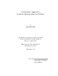
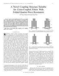
Figure 1 gives relative errors of approximation, (π ~ – π)/[π(1 – π)] 1/2 , where ~ π is the 

approximated power of F U , F T1 

, and F V by either the Muller-Peterson or the proposed 

algorithm and π is the exact power of U, T, and V given by Lee. Note that because 

[π(1 – π)] 1/2 ≤ 0.50, the relative error is at least twice that of the raw error, π ~ – π. 

_______________________________________________________________________ 

Figure 1. Relative errors of approximation for the Muller-Peterson (M-P) and the 

proposed methods for 18 cases studied by Lee (1971, Table 1). s = r A = 2, r C = {3, 5, 

7}, N – r X = 63. 

_______________________________________________________________________ 

The two F-based methods show accuracies that are quite acceptable for performing 

power analyses of proposed studies. For these cases, they give relative errors within 

±3%, with averages much less than that. The proposed method is seen to be biased 

positively for U and T 1 . As hypothesized above, the Muller-Peterson shows a tendency 

to underestimate power, but its overall accuracy seems slightly superior to the proposed 

method in these cases. We performed similar computations based on Lee's Table 2 and 

found the same pattern for s = r A = {3, 4} as we did for s = r A = 2. 

This encouraging assessment is limited in two respects. First, like other researchers 

of this topic, Lee was not concerned with methods for computing the power probabilities 

of F U , F T1 

, and F V , which are the test statistics generally used today. The powers of (say) 

U and F U surely diverge for lower N, though perhaps only slightly. As a practical matter, 

we would prefer an algorithm that gives more accurate powers for F U to one that gives 

more accurate powers for U. Second, the cases Lee created to investigate had powers 

much lower than are typically of interest. The largest power is 0.62, with the vast 

majority being less than 0.50. For problems of sample-size choice, one generally desires 

to have nominal powers of 0.80 or higher. We prefer 0.90. 

3.2 Monte Carlo Study 

For the reasons just stated, we performed a Monte Carlo study to assess how well we 

can compute the power of F U , F T1 

, F T2 

, and F V directly, for situations with meaningful 

10

. 

0.03 

0.02 

Relative Error of Approximation 

0.01 

0.00 

-0.01 

-0.02 

-0.03 

M-P 

Proposed 

M-P 

Proposed 

M-P 

Proposed 

F U 

F T1 

F V 

Figure 1.


power, π ≥ .80. 

Method and design. Because F T1 

has the simplest proposed nominal noncentral 

distribution, we used this to specify the particular non-null cases to simulate. For a given 

N, r X , r C , and r A , and a given nominal power, π T1 

= π 0 , we employed the SAS ® functions 

FINV and FNONCT to find λ 0 such that Prob[F(r C r A , ν (T 1) 

2 , λ 0 ) > F .05 (r C r A , ν (T 1) 

2 , 0)] = 

π 0 . For s > 1, we defined four different structures for the first s eigenvalues of Î ∗ , ƒ ∗ = 

{φ1 ∗ , φ2 ∗ ,..., φs ∗ }: 

Equal (E): ƒ ∗ = (λ 0 /N)s –1 {1, 1, ..., 1} 

Linear (L): ƒ ∗ = (λ 0 /N)[s(s + 1)/2] –1 {s, s – 1, ..., 1} 

Geometric (G): ƒ ∗ = (λ 0 /N)(2 s – 1) –1 {2 s-1 , 2 s–2 , ..., 1} 

Extreme (X): ƒ ∗ = (λ 0 /N){1, 0, ..., 0}. 

The sum of the roots, T ∗ = λ 0 /N, is the same for all four structures; thus, λ T = λ 0 , 

and the nominal power for F T1 

is π 0 . Though lower than π 0 , the nominal power for F T2 

is 

also the same under all four structures. On the other hand, λ U and λ V are affected by the 

structure of the eigenvalues. To keep π 0 fixed, the elements in ƒ ∗ must decrease with 

increasing N. 

We examined all four F statistics under the E, L, G, and X structures for N = {10, 20, 

30, 40, 50, 100}, r X = 4, r C = {2, 3}, r A = 3, and π 0 = {.80, 90}. This produced sets of s = 

2 and s = 3 cases that blanket a wide range of situations that are practical for power 

analyses. 

The experiment was performed using the IML ® matrix language of SAS. Each trial 

of a particular case proceeded as follows. Without loss of generality, Í ≡ I. H, an 

r A × r A noncentral Wishart matrix with r C degrees of freedom, was formed by first using 

the NORMAL function to generate an r C × r A matrix Z having independent rows that are 

N(0, I). Let M be the r C × r A matrix having elements m kk = (φk ∗ ) 1/2 , k = 1 to s, and 

m kk' = 0 for k ≠ k'. Then H = (Z + M)′(Z + M) is Wishart with noncentrality M′M, a 

diagonal matrix with elements {φ1 ∗ , φ∗ 2 ,..., φ∗ s , 0, ...0}. E, the r A × r A central Wishart 

matrix with N – r X degrees of freedom, was formed by generating an (N – r X ) × r A matrix 

Z having independent rows that are N(0, I) and computing E = Z′Z. The roots of E –1 H 

were then obtained and used to form F U , F T1 

, F T2 

, F V , which were compared to their 

respective nominal .05-level critical values. 5000 trials of each case where run, giving 

11


standard errors for each estimated true power of 0.0042 for π = 0.90 and 0.0057 for 

π = 0.80. We checked the accuracy of our programming and of IML’s NORMAL 

random number generator by simulating a full slate of s = r C = 1, r A = 3 cases and 

verifying that the obtained results fell within reasonable sampling errors of the known 

exact powers. 

_______________________________________________________________________ 

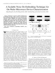
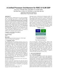
Figure 2. Proposed ( ) and Muller-Peterson ( ) approximations and estimated true 

powers ( ) as a function of eigenvalue structure and total sample size. αˆ is the 

estimated true Type-I error rate. r X = 4; r A = 3; s = r C = {2, 3}. 

_______________________________________________________________________ 

The results for π 0 = .90 are presented in Figure 2. The results for the linear structure 

for ƒ ∗ are not shown as they are identical to those of the geometric structure when s = 2 

and virtually the same when s = 3. Also, the pattern of results for π 0 = 0.80 were in 

complete accord with those for π 0 = 0.90. αˆ is the estimated true Type I error rate, the 

“power” at ƒ ∗ = 0. Note only that they are too low for F V when N ≤ 20. 

The power results reflect our theoretical conclusions and show a pattern consistent 

with those involving Lee's tables. The Muller-Peterson values are generally too low, 

whereas those obtained by the proposed method are somewhat high in some cases. The 

Muller-Peterson is better for F V with low N, but this is a “lucky” consequence of having 

the deflated αˆ values suppress the true power. In general, there is a clear tendency for 

the proposed method to give more accurate results. 

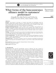
Figure 3 re-plots the results from the s = r A = r C = 3 cases to show the relative errors 

of approximation, (π ~ i – πˆ i )/[ πˆ i (1 – πˆ i )] 1/2 , where π ~ i is the proposed approximated 

power for a given F i statistic and πˆ i is the Monte Carlo estimate of F i ‘s true power. 

Cases were chosen to set ~ π T1 

= .90. The results show that F U has the most error-free 

approximations. For the equal and geometric (and linear) structures, the approximations 

for F T1 

, F U , and F V are positively biased, while those for F T2 

are negatively biased. 

Structure X induces the most error, with the proposed method performing best for F U and 

F T2 

. 

12

. 

proposed approximation M-P approximation estimated true power 

Power 

1.00 

0.90 

0.80 

0.70 

0.60 

0.50 

0.40 

ƒ: 

N: 

α: ˆ 

s = 2 

Wilks: F U 

E GX EGX EGX EGX EGX EGX 

10 20 30 40 50 100 

.048 .049 .051 .051 .050 .052 


1.00 

0.90 

0.80 

0.70 

0.60 

0.50 

0.40 

ƒ: 

N: 

α: ˆ 

s = 3 

Wilks: F U 

EGX EGX EGX EGX EGX EGX 

10 20 30 40 50 100 

.048 .043 .048 .060 .049 .048 


1.00 

0.90 

0.80 

0.70 

0.60 


1.00 

0.90 

0.80 

0.70 

0.60 

0.50 

Hotelling: F T1 

0.50 

0.40 

ƒ: EGX EGX EGX EGX EGX EGX 

0.40 

ƒ: 

N: 10 20 30 40 50 100 

N: 

α: ˆ .052 .058 .056 .055 .052 .054 

α: ˆ 


EGX 

10 

EGX 

20 

EGX 

30 

EGX 

40 

EGX 

50 

EGX 

100 

.058 .058 .056 .067 .055 .050 


1.00 

0.90 

0.80 

0.70 

0.60 

0.50 

0.40 

ƒ: 

N: 

α: ˆ 



10 20 30 40 50 100 

.046 .049 .052 .051 .050 .052 


1.00 

0.90 

0.80 

0.70 

0.60 

0.50 

0.40 

ƒ: 

N: 

α: ˆ 


E GX EGX EGX EGX EGX EGX 

10 20 30 40 50 100 

.045 .047 .047 .061 .049 .049 


1.00 

0.90 

0.80 

0.70 

0.60 

0.50 

0.40 

0.30 

0.20 

0.10 

ƒ: 

N: 

α: ˆ 

Pillai: F V 


10 20 30 40 50 100 

.024 .037 .045 .046 .046 .051 


1.00 

0.90 

0.80 

0.70 

0.60 

0.50 

0.40 

0.30 

0.20 

0.10 

ƒ: 

N: 

α: ˆ 

Pillai: F V 


10 20 30 40 50 100 

.020 .029 .039 .050 .044 .045 

Figure 2.


_______________________________________________________________________ 

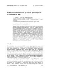
Figure 3. Estimated relative errors of approximation as a function of sample size and 

eigenvalue structure . s = r A = r C = 3; r X = 4; nominal power of .90 for F T1 

. 

_______________________________________________________________________ 

In conclusion, only when N is quite small (N ≤ 20) do we see any worrisome 

breakdown in accuracy. It is exceptional that this single, straightforward scheme 

performs so well over these four test statistics and four eigenvalue structures. 

4. COMPARING POWERS OF F U , F T1 

, F T2 

, and F V 

The proposed algorithm provides a convenient way to compare the powers of F U , 

F T1 

, F T2 

, and F V . Following Anderson (1984, p. 332), we frame our view by employing 

the coefficient of variation of ƒ ∗ , 

CV = 

s 

(φ * k – φ * 1/2 

Σ ) 2 /s 

k=1 

φ * , 

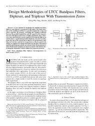
where φ * is their average. Figure 4 plots CV against the approximate powers computed 

using the proposed algorithm and the estimated true powers for the case of N = 50, 

r X = 4, and r C = r A = s = 3. The lines were constructed by computing the powers using 

ƒ ∗ = {T ∗ c, T ∗ (1 – c)/2, T ∗ (1 – c)/2} where T ∗ gives a power of π = 0.90 for F T1 

using 

α = .05. c varies between c = 1/3 (Structure E: CV = 0) and c = 1.0 (Structure X: 

CV = 2 ). Although the L and G structures do not have a pattern of {T e c, T e (1 – c)/2, 

T e (1 – c)/2}, their approximated powers fall right in line with those that do, as illustrated. 

Figure 4 demonstrates that these F i statistics have the same power relations that Anderson 

described for T, U, and V: As CV increases, F T1 

and F T2 

become more powerful than F U , 

which becomes more powerful than F V . Quite similar images appear when graphing the 

powers for all other combinations of r C = s = {2, 3}, π = {.80, .90}, and N = {50, 100}. It 

can be shown that under Structure E, λ T = λ V whenever s = r A . In addition, if s > 1, then 

ν (T 2) 

2 < ν (T 1) 

2 < ν 2 (V) , so it follows that the nominal power of F V exceeds that for F T1 

, 

which exceeds that for F T2 

in this case. We also note from the work of Schatzoff (1966) 

and Olson (1974) that Roy's statistic has greater power than these F i statistics under 

13

F U 

F T1 

F T2 

F V 

Estimated Relative Error of Approximation 

0.7 

0.6 

0.5 

0.4 

0.3 

0.2 

0.1 

0.0 

-0.1 

-0.2 

-0.3 

ƒ: 

EGX EGX EGX EGX 

N: 10 20 40 100 

Figure 3.


Structure X, but in general it has less power otherwise. 

_______________________________________________________________________ 

Figure 4. Nominal (lines) and estimated (points) powers of F V , F T1, 

F T2 

, and F V as a 

function of the coefficient of variation of φ ∗ 1 , φ∗ 2 , φ∗ 3 . N= 50; s = r A = r C = 3; r X = 4; 

nominal power of .90 for F T1 

. 

_______________________________________________________________________ 

5. THE q-GROUP PROBLEM, WITH EXAMPLE 

Most applications of the proposed method will be for power analyses in which q 

independent groups are compared with respect to P correlated measurements. This 

problem has a specific structure that we now exploit. An example follows. 

Let Ẍ be the q × r X essence model matrix formed by assembling the q unique rows 

of X (N × r X ; r X ≤ q). Ẍ is the collection of the q unique design points (e.g. the q 

groups) for the proposed study. If n j of the rows of X are equal to the j th row of Ẍ , define 

W to be the q × q diagonal matrix containing weights w j = n j /N. Thus (X′X) = 

N(Ẍ ′WẌ ), so that 

H ∗ = (CBA – Œ 0 )′[C(Ẍ ′WẌ ) -1 C′] -1 (CBA – Œ 0 ). 

Thus the eigenvalues of Î ∗ = (A′ÍA) –1 H ∗ , and hence the λ ∗ i , are based on the q defined 

design points (Ẍ ), the q sample-sizes weights (W); the conjectured values for the 

unknown effects (B), the conjectured common covariance matrix (Í), and the 

specification of the hypothesis (C, Œ 0 ). Importantly, λ ∗ i is not related to N. 

To illustrate the method briefly, consider a profile analysis arising from crossing a 3- 

level between-subjects factor, “Group,” with a 3-level within-subjects (repeated 

measures) factor, “Test.” The i th subject will provide three observations, y = [y i1 y i2 y i3 ] 

= [Test i1 Test i2 Test i3 ]. With N subjects total and taking the i th subject to be in the second 

group, the cell means formulation of Y = XB + ‰ is 

14

. 

ƒ: 

E L G X 

0.90 

F T1 


0.88 

0.86 

F T2 

F U 

0.84 

0.82 

F V 

0.80 

0.0 0.5 1.0 1.5 

Coefficient of Variation 

Figure 4.


⎡ y 11 y 12 y 13 ⎤ 

⎢ 

y 21 y 22 y 

⎥ 

⎢ 

23 ⎥ 

⎢ M M M ⎥ 

⎢ 

⎥ = 

⎢ y i1 y i2 y i3 ⎥ 

⎢ M M M ⎥ 

⎢ 

⎥ 

⎣y N1 y N2 y N3 ⎦ 

⎡1 0 0⎤ 

⎢ 

1 0 0 

⎥ 

⎢ ⎥⎡µ ⎢M M M⎥ 

11 µ 12 µ 13 ⎤ 

⎢ 

⎢ ⎥ µ 

⎢0 1 0 21 µ 22 µ 

⎥ 

⎢ 

23 ⎥ 

⎥ 

⎢M M M⎥⎣ 

⎢µ 31 µ 32 µ 33 ⎦⎥ 

⎢ ⎥ 

⎣0 0 1⎦ 

+ 

⎡ ε 11 ε 12 ε 13 ⎤ 

⎢ 

ε 21 ε 22 ε 

⎥ 

⎢ 

23 ⎥ 

⎢ M M M ⎥ 

⎢ 

⎥ . 

⎢ ε i1 ε i2 ε i3 ⎥ 

⎢ M M M ⎥ 

⎢ 

⎥ 

⎣ε N1 ε N2 ε N3 ⎦ 

Thus, Ẍ is the 3 × 3 identity matrix. The sample size weights are to be w 1 = .250, 

w 2 = .375, and w 3 = .375, giving the elements of the diagonal matrix W. Two scenarios 

for B are 

B (1) = 

97 110 97 

95 100 110 

102 95 105 and B (2) = 97 110 97 

100 100 100 

102 95 105 . 

The conjectured within-group standard deviations for y i1 , y i2 , and y i3 are 15, 20, and 15. 

Τhe within-group correlations are ρ 12 = 0.30, ρ 13 = 0.60, ρ 23 = 0.30. Thus 

Í = 15 0 0 

0200 

0 0 15 

1 .30 .60 

.30 1 .30 

.60 .30 1 

15 0 0 

0200 

0 0 15 

= 

225 90 135 

90 400 90 

135 90 225 . 

Comparing the test profiles across the three groups (the Group × Test interaction) can 

be specified with H 0 : CBA = 0 where 

C = 

0 1 −1 1 −1 0 and A = 1 1 

−1 0 

0 −1 . 

For B (1) , these specifications lead to ƒ ∗ = {.278, .134}, which is almost an 

linear/geometric eigenvalue structure. The primary noncentralities are λ ∗ U = .407, 

λ ∗ T = .412, λ∗ V = .403. For α = .05 and N = 48, the approximate powers are π U = .949, 

π T1 

= .951, π T2 

= .943, and π V = .947. For B (2) , ƒ ∗ = {.181, .004}, which is less than for 

B (1) and close to being an extreme eigenvalue structure. Accordingly, the primary 

noncentralities and powers (N = 48) are now lower and more varied: λ ∗ U = .178, 

λ ∗ T = .185, λ∗ V = .171; π U = .610, π T1 

= .630, π T2 

= .612, and π V = .590. For N = 96, the 

powers are π U = .923, π T1 

= .937, π T2 

= .929, and π V = .911. Note that the nominal Type 

II error rate for F V is 41% greater than for F T1 

, which should become the prescribed 

15


statistic for the written protocol if B (2) were the primary scenario. Other factors, 

especially robustness, might mitigate against such a decision. For instance, Olson (1974) 

concluded that V was the more robust statistic. 

6. CONCLUSION 

The value of the proposed strategy stems from several factors. (1) This is an all-inone 

method that relates directly and simply to the familiar F transforms of the U, T, and 

V statistics. These Fs are taken to be noncentral Fs with their usual degrees of freedom. 

Computing their noncentrality parameters is isomorphic to computing the F statistics on 

population values instead of sample values. As described fully in O’Brien and Muller 

(1993), exploiting the correspondence between a familiar test statistic and its 

noncentrality parameter gives intuition and pragmatism to power analysis. This is not the 

case for the more abstruse methods that have been proposed over the years for numerous 

special cases involving U, T, and V directly (see Krishnaiah, 1978). (2) The method 

gives exact powers when applied to any test having s = 1. (3) For s > 1, the method 

affords a unifying set of asymptotic results that support its large-sample correctness 

across the various F transforms. (4) For s > 1, but with smaller sample sizes, the 

empirical work summarized and graphed above shows the method to be sufficiently 

accurate for almost all applied work. Although methods that are more exact have been 

developed for special situations involving U, T and V, such work does not extend to the 

approximate F U , F T1 

, F T2 

, and F V statistics being used so predominately today. 

In conclusion, we offer a way to compute power probabilities for the multivariate 

general linear hypothesis that is simple, general, and accurate. We hope these qualities 

motivate statistical planners to perform power analyses that are more congruent with the 

multivariate hypotheses they propose to test. 

16


References 

Agresti, A. (1990), Categorical Data Analysis , New York: John Wiley. 

Anderson, T. W. (1984), An Introduction to Multivariate Statistical Analysis (2nd ed.), 

New York: Wiley. 

Barton, C. N. and Cramer, E. C. (1989), “Hypothesis Testing in Multivariate Linear 

Models with Randomly Missing Data,” Communications in Statistics—Simulation 

and Computations, 18, 875-895. 

Bartlett, M. S. (1939), “A Note of Tests of Significance in Multivariate Analysis,” 

Proceedings of the Cambridge Philosophical Society, 35, 180-185. 

Hughes, J. T. and Saw, J. G. (1972), “Approximating the Percentage Points of Hotelling's 

Generalized T 2 0 Statistic,” Biometrika, 59, 224-226. 

Krishnaiah, P. R. (1978), “Some Recent Developments on Real Multivariate 

Distributions,” in Developments in Statistics (Vol.1), ed. P. R. Krishnaiah, New 

York: Academic Press, pp. 135-169. 

Kulp, R. W. and Nagarsenker, B. N. (1984), “An Asymptotic Expansion of the NonNull 

Distribution of Wilks Criterion for Testing the Multivariate Linear Hypothesis,” 

Annals of Statistics, 12, 1576-1583. 

Lee, Y. S. (1971), “Asymptotic Formulae for the Distribution of a Multivariate Test 

Statistic: Power Comparisons of Certain Multivariate Tests,” Biometrika, 58, 647- 

651. 

McKeon, J. J. (1974), “F Approximations to the Distribution of Hotelling's T 2 0 ,” 

Biometrika, 61, 381-383. 

Muller, K. E. and Barton, C. N. (1989), “Approximate Power for Repeated-Measures 

ANOVA Lacking Sphericity,” Journal of the American Statistical Association, 84, 

549-555. 

Muller, K. E., LaVange, L. M., Ramey, S. L., and Ramey, C. T. (1992), “Power 

Calculations for General Linear Multivariate Models Including Repeated Measures 

Applications,” Journal of the American Statistical Association, 87, 1209-1226. 

Muller, K. E. and Peterson, B. L. (1984), “Practical Methods for Computing Power in 

Testing the Multivariate General Linear Hypothesis,” Computational Statistics & 

Data Analysis, 2, 143-158. 

Nanda, D. N. (1950), “Distribution of the Sum of Roots of a Determinantal Equation 

Under a Certain Condition,” Annals of Mathematical Statistics, 21, 432-439. 

17


O'Brien, R. G. (1986), “Using the SAS System to Perform Power Analysis for Log- 

Linear Models,” in Proceedings of the Eleventh Annual SAS Users Group 

International (SUGI), Cary, NC: SAS institute, 778-784. 

O'Brien, R. G. and Muller, K. E. (1993), “Unified Power Analysis for t-Tests through 

Multivariate Hypotheses,” in Edwards, L. K. (ed.), Applied Analysis of Variance in 

Behavioral Science, New York: Marcel Dekker, 297-344. 

Olson, C. L. (1974), “Comparative Robustness of Six Tests in Multivariate Analysis of 

Variance,” Journal of the American Statistical Association, 69, 894-908. 

Pillai, K. C. S. (1955), “Some New Test Criteria in Multivariate Analysis,” Annals of 

Mathematical Statistics, 26, 117-121. 

Pillai, K. C. S. and Mijares, T. A. (1959), “On the Moments of the Trace of a Matrix and 

Approximations to its Distribution,” Annals of Mathematical Statistics, 30, 1135- 

1140. 

Pillai, K. C. S. and Samson, P., Jr. (1959), “On Hotelling's Generalization of T 2 ,” 

Biometrika, 46, 160-168. 

Rao, C. R. (1951), “An Asymptotic Expansion of the Distribution of Wilks's Criterion, 

Bulletin of the International Statistical Institute, 33, 177-180. 

Searle, S. R. (1971), Linear Models, New York: John Wiley. 

Searle, S. R. (1982), Matrix Algebra Useful for Statistics, New York: John Wiley. 

Seber, G. A. F. (1984), Multivariate Observations, New York: John Wiley. 

Schatzoff, M. (1966), “Sensitivity Comparisons Among Tests of the General Linear 

Hypothesis,” Journal of the American Statistical Association, 61, 415-435. 

Sugiura, N. and Fujikoshi, Y. (1969), “Asymptotic Expansions of the Non-Null 

Distributions of the Likelihood Ratio Criteria for the Multivariate Linear Hypothesis 

and Independence,” Annals of Mathematical Statistics, 40, 942-952. 

van der Merwe, L. and Crowther, N. A. S. (1984), “An Approximation to the Distribution 

of Hotelling's Generalized T 2 0 -Statistic,” South African Statistical Journal, 18, 68- 

90. 

Wilks, S. S. (1932), “Certain Generalizations in the Analysis of Variance,” Biometrika, 

24, 471-494. 

18

Pragmatic, Unifying Algorithm Gives Power Probabilities for ...

You also want an ePaper? Increase the reach of your titles

Delete template?

Save as template?