Pragmatic, Unifying Algorithm Gives Power Probabilities for ...
Pragmatic, Unifying Algorithm Gives Power Probabilities for ...
Pragmatic, Unifying Algorithm Gives Power Probabilities for ...
You also want an ePaper? Increase the reach of your titles
YUMPU automatically turns print PDFs into web optimized ePapers that Google loves.
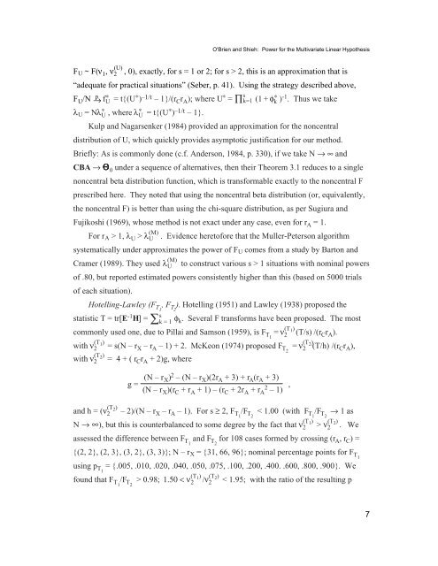
O'Brien and Shieh: <strong>Power</strong> <strong>for</strong> the Multivariate Linear Hypothesis<br />
F U ~ F(ν 1 , ν 2 (U) , 0), exactly, <strong>for</strong> s = 1 or 2; <strong>for</strong> s > 2, this is an approximation that is<br />
“adequate <strong>for</strong> practical situations” (Seber, p. 41). Using the strategy described above,<br />
F U /N → p f ∗ U = t{(U∗ ) –1/t – 1}/(r C r A ); where U ∗ s<br />
= ∏k=1 (1 + φk ∗ )-1 . Thus we take<br />
λ U = Nλ ∗ U , where λ ∗ U = t{(U ∗ ) –1/t – 1}.<br />
Kulp and Nagarsenker (1984) provided an approximation <strong>for</strong> the noncentral<br />
distribution of U, which quickly provides asymptotic justification <strong>for</strong> our method.<br />
Briefly: As is commonly done (c.f. Anderson, 1984, p. 330), if we take N → ∞ and<br />
CBA → Œ 0 under a sequence of alternatives, then their Theorem 3.1 reduces to a single<br />
noncentral beta distribution function, which is trans<strong>for</strong>mable exactly to the noncentral F<br />
prescribed here. They noted that using the noncentral beta distribution (or, equivalently,<br />
the noncentral F) is better than using the chi-square distribution, as per Sugiura and<br />
Fujikoshi (1969), whose method is not exact under any case, even <strong>for</strong> r A = 1.<br />
For r A > 1, λ U > λ (M)<br />
U . Evidence hereto<strong>for</strong>e that the Muller-Peterson algorithm<br />
systematically under approximates the power of F U comes from a study by Barton and<br />
Cramer (1989). They used λ (M)<br />
U to construct various s > 1 situations with nominal powers<br />
of .80, but reported estimated powers consistently higher than this (based on 5000 trials<br />
of each situation).<br />
Hotelling-Lawley (F T1<br />
, F T2<br />
). Hotelling (1951) and Lawley (1938) proposed the<br />
statistic T = tr[E -1 s<br />
H] = ∑k = 1<br />
φ k . Several F trans<strong>for</strong>ms have been proposed. The most<br />
commonly used one, due to Pillai and Samson (1959), is F T1<br />
= ν (T 1)<br />
2 (T/s) /(r C r A ).<br />
with ν (T 1)<br />
2 = s(N – r X – r A – 1) + 2. McKeon (1974) proposed F T2<br />
= ν (T 2)<br />
2 (T/h) /(r C r A ),<br />
with ν (T 2)<br />
2 = 4 + ( r C r A + 2)g, where<br />
g = (N – r X) 2 – (N – r X )(2r A + 3) + r A (r A + 3)<br />
(N – r X )(r C + r A + 1) – (r C + 2r A + r A<br />
2<br />
– 1)<br />
,<br />
and h = (ν (T 2)<br />
2 – 2)/(N – r X – r A – 1). For s ≥ 2, F T1<br />
/F T2<br />
< 1.00 (with F T1<br />
/F T2<br />
→ 1 as<br />
N → ∞), but this is counterbalanced to some degree by the fact that ν (T 1)<br />
2 > ν (T 2)<br />
2 . We<br />
assessed the difference between F T1<br />
and F T2<br />
<strong>for</strong> 108 cases <strong>for</strong>med by crossing (r A , r C ) =<br />
{(2, 2}, (2, 3}, (3, 2}, (3, 3)}; N – r X = {31, 66, 96}; nominal percentage points <strong>for</strong> F T1<br />
using p T1<br />
= {.005, .010, .020, .040, .050, .075, .100, .200, .400. .600, .800, .900}. We<br />
found that F T1<br />
/F T2<br />
> 0.98; 1.50 < ν (T 1)<br />
2 /ν (T 2)<br />
2 < 1.95; with the ratio of the resulting p<br />
7


