COMPIT 2010 in Gubbio - TUHH

9 th International Conference on
Computer and IT Applications in the Maritime Industries
COMPIT’10
Gubbio, 12-14 April 2010
Edited by Volker Bertram
1

Sponsored by
www.GL-group.com www.futureship.net www.friendship-systems.com
www.onrglobal.navy.mil
www.aveva.com
www.foran.es
www.shipconstructor.com
www.napa.fi
www.ssi.tu-harburg.de
This work relates to a Department of the Navy Grant issued by the Office of Naval Research
Global. The United States Government has a royalty-free license throughout the world in all
copyrightable material contained herein.
2

9 th International Conference on Computer and IT Applications in the Maritime
Industries:, Gubbio, 12-14 April 2010, Hamburg, Technische Universität Hamburg-Harburg,
2010, ISBN 978-3-89220-649-1
© Technische Universität Hamburg-Harburg
Schriftenreihe Schiffbau
Schwarzenbergstraße 95c
D-21073 Hamburg
http://www.tuhh.de/vss
3

Index
Ahmad F. Ayob, Tapabrata Ray, Warren F. Smith 7
A Framework for Scenario-Based Hydrodynamic Design Optimization of Hard Chine
Planing Craft
Volker Bertram, Patrick Couser 20
Aspects of Selecting the Appropriate CAD and CFD Software
Markus Druckenbrod, Jochen Hundemer, Moustafa Abdel-Maksoud, Max Steden 30
Optimisation of Single and Multi-Component Propulsors
Valery Mrykin, Vyacheslav Lomov, Sergey Kurnosov, Manucher Dorri 39
Training Complex for Training Submarine Motion Control Skills on the Basis of Virtual
Dynamic Systems
Jose Marcio Vasconcellos 48
Ship Structural Optimization under Uncertainty
Jean-David Caprace, Frédéric Bair, Philippe Rigo 56
Multi-Criterion Scantling Optimisation of Passenger Ships
Isabelle Toulgoat, Pierre Siegel, Yves Lacroix, Julien Botto 65
Operator Decision Modeling in a Submarine
Matteo Diez, Daniele Peri 76
Two-stage Stochastic Programming Formulation for Ship Design Optimization under
Uncertainty
Kunihiro Hamada, Yoshifumi Takanobu, Kesavadev Varikkattu 90
Development of Ship Design Support System in Consideration of Uncertainty in Product
Information
Anthony S. Daniels, Morgan C. Parker, David J. Singer 99
Effects of Uncertainty in Fuzzy Utility Values on General Arrangements Optimization
Verónica Alonso, Carlos González 113
The Challenge in Hull Structure Basic Design: From Traditional 2D Drawings to 3D Early
Product Model
Robert Hekkenberg 124
“The Virtual Fleet” – Use of Extended Conceptual Design Data for Trend Analysis of
Inland Ship Characteristics
Ralf Tschullik, Hannes Prommer, Pentscho Pentschew, Patrick Kaeding 132
A Concept of Topological Optimization for Bow Structures
Monique Chyba, Michael Andonian, Dario Cazzaro, Luca Invernizzi 139
Trajectory Design for Autonomous Underwater Vehicles for Basin Exploration
Marco Bibuli, Massimo Caccia, Renato Robino, William Bateman, Thomas Vögele, Alberto
Ortiz, Leonidas Drikos, Albena Todorova, Ioanins Gaviotis, Francesco Spadoni, Vassiliki
Apostolopoulou
Robotic Tools to Assist Marine Inspection: The MINOAS Approach
152
4

Frank Borasch 166
A Digital Planning Tool for Outfitting: “DigiMAus”
George Bruce, Mike Evans 176
Reducing Management Software Costs
Thomas Koch 182
Validation and Quality Control of Design and Production Information - Applying Rule
Based Data Mining and Business Intelligence Concepts to Engineering
Roope Kotiranta 194
Extended usage of a Modern Product Model in Finite Element Analysis
Hermann Lödding, Axel Friedewald, Lars Wagner 203
Rule-Based Resource Allocation – An Approach to Integrate Different Levels of Planning
Detail in Production Simulation
Tomasz Abramowski 213
Combining Artificial Neural Networks and Simulated Annealing Algorithm for Increasing
Ship Transport Efficiency
Tomasz Abramowski, Tadeusz Szelangiewicz, Katarzyna śelazny 221
Developing of a Computer System Aiding the Determination of Mean Long-Term Service
Speed
Reyhane Rostami, MohammadReza Matash Boroujerdi 235
Data Mining to Enhance the Throughput of Container Ports
Rolf Oetter 243
Revitalizing Brazil’s Shipbuilding Industry - A Case Study
Darren Larkins 249
Practical Applications of Design for Production
Karel Wagner, Alain Wassink, Bart van Oers, Hans Hopman 259
Modeling Complex Vessels for Use in a 3D Packing Approach: An Application to
Deepwater Drilling Vessel Design
Thomas DeNucci, Hans Hopman 273
Optimization-Based Approach to Rationale Capturing in Ship Design
Benedict Boesche 285
Improvement of Interoperability between Yards and Equipment Suppliers
David J. Andrews, Tim P. McDonald, Richard G. Pawling 290
Combining the Design Building Block and Library Based Approaches to improve
Exploration during Initial Design
Dirk Steinhauer 304
GeneSim - Development of a Generic Data Model for Production Simulation in Shipbuilding
Tommi Kurki 311
Utilization of Integrated Design and Mesh Generation in Ship Design Process
Marcus Bole
Interactive Hull Form Transformations using Curve Network Deformation
319
5

Stefan Harries, Florian Vesting 335
Aerodynamic Optimization of Superstructures and Components
Andrea Caiti, Andrea Munafò 348
AUV Networks for Adaptive Area Coverage with Reliable Acoustic Communication Links
Heikki Hansen, Malte Freund 356
Assistance Tools for Operational Fuel Efficiency
Bart van Oers, Douwe Stapersma, Hans Hopman 367
A 3D packing Approach for the Early Stage Configuration Design of Ships
Shi Wei, Hugo Grimmelius 382
Comparison of Modeling Techniques for Simulation of Fuel Consumption of Dredgers
Nick Danese 396
Ship CAD Systems - Past, Present and Possible Future
Océane Balland, Siri Solem, Arnulf Hagen, Stein Ove Erikstad 409
A Decision Support Framework for the Concurrent Selection of Multiple Air Emission
Controls
Edwin R. Galea, Rob Brown, Lazaros Filippidis, Steven Deere 424
The SAFEGUARD project: Collection and Preliminary Analysis of Assembly Data for Large
Passenger Vessels at Sea
Henrique M. Gaspar, Eivind Neumann-Larsen, Audun Grimstad, Stein Ove Erikstad 434
Efficient Design of Advanced Machinery Systems for Complex Operational Profiles
Martin-Christoph Wanner, Ralf Bohnenberg, Ulrich Kothe, Jan Sender, Reiner Czarnietzki 449
Development of a Methodology for Calculating Production Times based on Parameters
Igor Mizine, Bruce Wintersteen 458
Multi-Level Hierarchical System Approach in Computerized Ship Design
Christian Cabos, Uwe Langbecker, Wiegand Grafe 478
Hull Maintenance Based on a 3D Model
David Thomson 491
Requirements of a Common Data Model for Total Ship Lifecycle Data Management
Index of authors 505
Call for Papers COMPIT’11
6

A Framework for Scenario-Based Hydrodynamic Design Optimization of
Hard Chine Planing Craft
Abstract
Ahmad F. Ayob, UMT, Terengganu/Malaysia, z3237562@student.adfa.edu.au
Tapabrata Ray UNSW@ADFA, Canberra/Australia, t.ray@adfa.edu.au
Warren F. Smith UNSW@ADFA, Canberra/Australia, w.smith@adfa.edu.au
An optimization framework for the design of hard chine planing craft incorporating resistance,
seakeeping and stability considerations is presented. The proposed framework consists of a surface
information retrieval module, a geometry manipulation module and an optimization module backed
by standard naval architectural performance estimation tools. Total resistance comprising calm
water resistance and added resistance in waves is minimized subject to constraints on displacement,
stability and seakeeping requirements. Three optimization algorithms are incorporated in the
optimization module: Non-dominated Sorting Genetic Algorithm (NSGA-II), Evolutionary Algorithm
with Spatially Distributed Surrogates (EASDS), and Infeasibility Driven Evolutionary Algorithm
(IDEA). The individual performance of each algorithm is reported. The proposed framework is
capable of generating the optimum hull form, which allows for a better estimate of performance
compared to methods that generate only the optimum principal dimensions. The importance and
effects of the vertical impact acceleration constraint on manned and unmanned missions are also
discussed.
Nomenclature
B Beam (m) L Length (m)
C v Speed coefficient LCB Longitudinal centre of buoyancy (m)
Disp. Displacement (kg) R A Added resistance (N)
Fn Froude number R C Calm water resistance (N)
GM Metacentric height (m) R T Total resistance (N)
H 1/3 Significant wave height (m) T Draft (m)
I e Half angle of entrance (degrees) Vol. Displaced volume (m 3 )
I a Vertical impact acceleration (g)
1. Introduction
Ship design involves the practice of satisfying requirements based on a vessel’s intended tasks and
rationalization, Schneekluth and Bertram (1998). The design of a ship should meet statutory
requirements, mission requirements, economic criteria, safety requirements and so on. The choices of
main dimensions of the ship affect the hydrostatic and hydrodynamic performance of the ship such as
its resistance and response in the seaway. Ship design optimization allows the tradeoff between
various performance requirements and is an indispensable element of modern day design processes.
Consideration of seakeeping performance during the phase of design has been reported in a number of
recent studies. Sarioz and Narli (2005) presented an example of seakeeping assessment under various
vertical acceleration regimes outlined in ISO 2631, Mason and Thomas (2007) illustrated the use
Computational Fluid Dynamics (CFD) and Genetic Algorithm (GA) for the optimization of
International America’s Cup Class (IACC) yachts, Peri and Campana (2003) designed a naval
surface combatant with total resistance and seakeeping considerations. Other examples involving
multiple design aspects i.e. resistance, seakeeping, cost and safety optimization based on specific
scenarios have been presented by Smith (1992), Ray (1995), Ganesan (1999), Neti (2005) and
Berseneff et al. (2009).
Most of the above studies focused on displacement crafts and there are only a handful studies dealing
with planing crafts. Minimization of calm water resistance for planing crafts appears in Almeter
(1995) and Mohamad Ayob et al. (2009). Presented in this paper is a scenario based hydrodynamic
7

optimization of planing craft in seaway operations. An integrated approach is taken that
simultaneously considers resistance and motions in a seaway. A number of efficient optimization
algorithms are employed for solving the problems posed. The Non-dominated Sorting Genetic
Algorithm-II (NSGA-II) by Deb et al. (2002) is incorporated in the planing craft optimization
framework. In addition to NSGA-II, a surrogate assisted optimization scheme (referred here as
EASDS) by Isaacs et al. (2007) and an Infeasibility Driven Evolutionary Algorithm (IDEA) Ray et al.
(2009) is incorporated for increased efficiency.
In order to support design optimization of planing craft, the underlying framework should:
1. allow easy incorporation of different scenarios, design criteria etc. with alternate analysis
modules providing different levels of fidelity;
2. allow shape representation and manipulation that is able to generate different variants of hull
forms with the required fairness and chine definitions; and
3. include an optimization method that is capable of dealing with single and multi-objective
optimization problems with constraints. Furthermore, since the performance evaluations are
computationally expensive, the optimization algorithms employed should be efficient.
The proposed framework is built using a modular concept with the Microsoft ® COM interface as the
underlying communication platform between applications. A modular design in any optimization
framework opens the possibility of conducting more complex analysis, Ray (1995), where other
optimization schemes and high fidelity multidisciplinary analysis tools can be added and executed for
comparative purposes. A number of researchers have discussed helpful proposals for integration of
different tools within a ship design framework. Neu et al. (2000) applied Microsoft ® COM interface in
containership design optimization. Mohamad Ayob et al. (2009) used Maxsurf Automation, Maxsurf
(2007) (a form of Microsoft ® COM interface) for planing craft design optimization. Abt et al. (2009)
presented a broader aspect of integration between tools, including integration of in-house and
commercial codes using XML files, generic templates and Microsoft COM interface.
2. Optimization framework components
The optimization framework proposed in this paper consists of three applications namely Matlab,
Microsoft ® Excel and Maxsurf. Maxsurf Automation Library built upon Microsoft ® COM interface is
used as a medium of communication (inter-process) between applications. Presented in Fig. 1 is a
generic sequence diagram to illustrate the workflow of the current optimization framework. The interprocess
communication is initialized with the selection of principal dimensions (L, B, T) by the
optimizer module in Matlab. Parametric transformation is invoked to generate a candidate hull
followed by evaluation of the hydrostatics and calm water resistance of the candidate hull in Maxsurf
using the methods of Savitsky (1964). Finally the seakeeping performance is evaluated using the
Savitsky and Koelbel (1993) method. This completes one workflow loop. The detail flowchart on the
optimization framework is presented in Fig. 2 with further discussion of this provided in subsequent
sections.
Fig. 1: Inter-process communication flow between applications
8

Fig. 2: Detail flowchart on the optimization framework
2.1. Geometry tools
The geometry tools consist of a surface information retrieval module and a geometry manipulation
module. Shown in Fig.2, the surface information retrieval module is employed to generate B-spline
representation of the hull while the geometry manipulation module changes the shape of the hull
based on principal dimensions given by the optimizer.
The formulation of surface information module is based on the inverse B-spline method, Rogers and
Adams (1990). A set of known surface (offset) data is used to determine the defining polygon net for a
B-spline surface that best interpolates the data. This method is further expanded to yield a
representation of a hard chine form that normally represents a planing craft, Mohamad Ayob et al.
(2009). Three B-spline surfaces defined by their own respective polygon nets station-wise with the
exclusion of the bow are connected to produce hard chines of the planing craft as shown in Fig. 3.
Fig. 3: Three-dimensional view of the planing craft with governing control points
9

Since the work of Lackenby (1950), the parametric transformation method has been used widely by
naval architects to modify the form parameters of an existing parent hull form. While LCB and C p
values of the resulting hull can be maintained when the hull sections are moved forward and aft, the
displacement value of the hull is changed in the process. In this study the parametric transformation
module of Maxsurf is considered as it offers the capability to produce new candidate hull forms while
maintaining the displacement and coefficient values of the parent hull, Maxsurf (2007). Control points
defining the non-uniform rational B-splines surface (NURBS) of the ship are moved in a smooth
fashion producing an acceptable fair surface of the resulting hull. An elaborate discussion on the
development of Maxsurf parametric transformation can be found in Mason and Thomas (2007).
2.2. Resistance estimation module
Calm water resistance estimation of planing craft is bounded by certain validation criteria. The details
of the range of validation is discussed in the work of Savitsky (1964) and Savitsky and Ward Brown
(1976) and in this study will be employed as constraints to the optimization problem. The details of
the planing craft studied in this paper are presented in Table I. As discussed in Savitsky and Ward
Brown (1976), a craft is in full planing mode for speed coefficient C v > 1.5. In this regime, the
resulting dynamic forces cause a significant rise of the center of gravity, positive trim, emergence of
the bow and the separation of the flow from the hard chines.
2.3. Seakeeping estimation technique
Table I: Characteristics of the planing craft
Displacement
7204.94 kg
Length
10.04 m
Beam
2.86 m
Draft
0.7 m
Metacentric height (GM) 2.0 m
Speed
20.81 kts
C V = V/(g x B) 1/2 2.02
The method described in Section 2.2 is suitable for calm water resistance. However, an additional
formulation is required in order to calculate the total resistance, R T of the planing craft operating in a
seaway. Fridsma's (1971) experimental tank test data on planing craft operating in rough water has
been reworked by Savitsky and Ward Brown (1976) in a form of equations suitable for computer
programming. The estimation modules discussed serve as mathematical model in order to search for
the optimum design inside the framework. Total resistance and average vertical impact acceleration
over irregular waves having energy spectrum of Pierson-Moskovitz is used in this study.
2.4. Maxsurf Automation
Maxsurf Automation is an interface that provides extensive possibilities of integration between
different naval architectural tools, whether developed in-house or commercially, Maxsurf (2007). The
automation library is built upon the Microsoft ® COM framework, thus allowing automation of calls
between compatible applications.
2.5. Optimization algorithms
In this framework, three state of the art optimization algorithms have been used namely NSGA-II,
EASDS and IDEA. The algorithms are written in Matlab and integrated via the Microsoft ® COM
interface discussed earlier.
An elitist, population-based, zero-order, stochastic algorithm known as the Non-dominated Sorting
Genetic Algorithm II (NSGA-II) is used as the underlying optimization algorithm. NSGA-II is known
10

to be able to solve a wide range of engineering problems. The algorithm starts with a population of
solutions that undergo crossover and mutation to generate offsprings. The current population and
current offspring population are sorted based on non-domination and only the best N individuals are
selected, where N is the population size. For complete details the readers are referred to the work of
Deb et al. (2002).
Most forms of evolutionary algorithm including NSGA-II require the evaluation of numerous
candidate solutions prior to its convergence, thus their applicability is restricted for computationally
expensive optimization problems. In order to overcome the problem of lengthy computational time,
surrogates or approximations can be employed. In this study an evolutionary algorithm with spatially
distributed surrogates (EASDS) is employed. The evolutionary algorithm is embedded with multiple
surrogates such as the ordinary response surface method (ORSM), the normalized response surface
method (RSM), the ordinary radial basis function (ORBF), the normalized radial basis function
(RBF) and the kriging method (DACE). The algorithm performs actual analysis for the initial
population followed by periodical evaluations in every few generations. A new candidate solution is
predicted by the surrogate model with the least prediction error in the neighbourhood of that point.
The complete details of the algorithm are explained in Isaacs et al. (2007).
Solutions to real-life constrained optimization problems lie often on constraint boundaries. In reality,
a designer is often interested in looking at the solutions that might be marginally infeasible. Most
optimization algorithms including NSGA-II intrinsically prefer a feasible solution over an infeasible
solution during the search. However, some recent works suggest that effectively utilizing the
marginally infeasible solutions during the search can expedite the rate of convergence. To this effect,
Infeasibility Driven Evolutionary Algorithm (IDEA) by Ray et al. (2009) is also used in this study.
3. Numerical experiments
In this section, the definition of the seaway operability condition, optimization problem formulation
and results for various scenarios are presented. The significance of various design criteria are further
discussed in the following subsections.
3.1. Definition of the seaway and operability condition
The case study refers to a design around coastal waters of Visakhapatnam in India. The wind speed
data for the above location is obtained from Shreeram and Rao (2005). An approximate value of the
significant wave height, H 1/3 data is estimated along the range of 12 nautical miles (22 km) and is
presented in Table II. The location of interest is shown in Fig. 4.
Table II: Chosen significant wave height data for numerical experiment
Wind Speed Sea State Code Significant Wave Height
4 m/s 1 0.4 m
5 m/s 2 0.6 m
6 m/s 2 0.8 m
7 m/s 3 1.1 m
Habitability of a craft can be assessed by means of ISO (1985) where vertical acceleration, exposure
time and frequency are linked together to yield the seakeeping criteria. An example of its applicability
was illustrated by Sarioz and Narli (2005).
11

Fig.4: Territorial waters of India near Visakhapatnam, 12 nautical miles from the coastal line
3.2. Optimization problem formulation
The optimization problem is posed as the identification of a planing craft with minimum total
resistance subject to the constraints on displacement, stability (transverse metacentric height) and
impact acceleration corresponding to the operational sea-states. The planing craft used in this study
represents a craft similar to U.S. Coast Guard (USCG) Surf Rescue Boat (30-foot SRB) (Halberstadt
(1987)). The ship is designed to operate in sea up to 3 m waves, with a maximum speed of 30 knots.
The seaway scenarios are expressed in Table II by significant wave heights H 1/3 assuming Pierson-
Moskovitz spectra. The objective functions and constraints are listed below, where subscripts B, I, T,
C and A resemble basis hull, candidate hull, total resistance, calm water resistance and added
resistance due to waves, respectively.
Minimize:
f = R T , where R T = R C + R A
Design variables: 9m

acceleration. Similar results were obtained for studies conducted at sea state 2. In the case of designs
under sea state 3 conditions as shown in Fig. 5(b) and Table V to VII, the basis hull has vertical
impact acceleration larger than 2g violating the constraint. Runs of all the algorithms are able to
achieve feasible designs while satisfying the constraint on impact acceleration, though at a cost of an
increased R T .
1.36
1.34
EASDS
IDEA
NSGA-II
2.15
EASDS
IDEA
NSGA-II
1.32
2.1
Total Resistance
1.38 x 104 Function Evaluations
1.3
1.28
1.26
Total Resistance
2.2 x 104 Function Evaluations
2.05
2
1.24
1.95
1.22
1.2
1.9
1.18
0 100 200 300 400 500 600
1.85
0 100 200 300 400 500 600
(a) Sea-state 1 (H 1/3 = 0.4m)
(b) Sea-state 3 (H 1/3 = 1.1m)
Fig. 5: Optimization progress plot of ship with vertical impact acceleration constraint
1.36
1.34
1.32
EASDS
IDEA
NSGA-II
1.36
1.34
EASDS
IDEA
NSGA-II
Total Resistance
1.38 x 104 Function Evaluations
1.3
1.28
1.26
Total Resistance
1.38 x 104 Function Evaluations
1.32
1.3
1.28
1.24
1.22
1.26
1.2
1.24
1.18
0 100 200 300 400 500 600
(a) Sea-state 1 (H 1/3 = 0.4m)
1.22
0 100 200 300 400 500 600
(b) Sea-state 2 (H 1/3 = 0.6m)
1.295
EASDS
IDEA
NSGA-II
1.335
EASDS
IDEA
NSGA-II
1.29
1.33
Total Resistance
1.3 x 104 Function Evaluations
1.285
1.28
Total Resistance
1.34 x 104 Function Evaluations
1.325
1.32
1.275
1.315
1.27
0 100 200 300 400 500 600
1.31
0 100 200 300 400 500 600
(c) Sea-state 2 (H 1/3 = 0.8m)
(d) Sea-state 3 (H 1/3 = 1.1m)
Fig. 6: Optimization progress plot of ship without vertical impact acceleration constraint
13

The value of impact acceleration and R T of the basis hull at sea state 3 is 2.11g and 13545.90 N
respectively, while all optimized designs have impact acceleration 1.5g and R T of 21830.67 N,
21829.52 N and 21833.40 N for NSGA-II, EASDS and IDEA, respectively. The optimized hull forms
found by the optimizers have similar characteristics where larger values of L, B and T result in a larger
displacement in order to satisfy the vertical impact acceleration constraint. The details on the
dimensions are highlighted in Tables V to VII.
The results for the optimization without the impact acceleration constraint are shown in Fig. 6. Total
resistance values of the best run of each algorithm (EASDS, IDEA and NSGA-II) are plotted against
function evaluations for typical sea states of 1, 2 and 3. In all sea-states, EASDS was able to
converge faster than IDEA and NSGA-II. One can observe by comparing Fig. 5(b) and Fig. 6(d) that
an increase of R T as high as 61% is necessary to satisfy the impact acceleration constraint, as
compared to a reduction by 2.97% when the impact acceleration constraint is ignored.
Shown in Fig. 7 is the progress for the median designs obtained using NSGA-II, EASDS and IDEA
for sea-state 1. Given the approximately same number of function evaluations, IDEA converges faster
than the other two algorithms while EASDS converges better than NSGA-II. A more comprehensive
comparison between algorithms can be observed in Tables III and IV where the best values of median
designs at all sea-states are depicted in bold type. EASDS consistently performs better than NSGA-II
and IDEA in solving the minimization problem with the impact acceleration constraint, while IDEA
outperforms the other two algorithms for the problem without the impact acceleration constraint.
1.38 x 104 Function Evaluations
1.36
1.34
EASDS
IDEA
NSGA-II
1.32
Total Resistance
1.3
1.28
1.26
1.24
1.22
1.2
1.18
0 100 200 300 400 500 600
Fig 7: Median design obtained using EASDS, IDEA and NSGA-II
Table III: Comparison between R T (N) of median designs with I a constraint
Sea-state 1 (0.4m) Sea-state 2 (0.6m) Sea-state 2 (0.8m) Sea-state 3 (1.1m)
NSGA-II 12060.96 12460.96 13858.59 21844.52
EASDS 11955.90 12415.75 13314.61 21842.02
IDEA 11933.19 12549.24 13709.51 21871.29
Table IV: Comparison between R T (N) of median designs without I a constraint
Sea-state 1 (0.4m) Sea-state 2 (0.6m) Sea-state 2 (0.8m) Sea-state 3 (1.1m)
NSGA-II 12065.10 12460.96 12968.60 13506.20
EASDS 11999.19 12415.75 12916.91 13468.44
IDEA 11962.04 12445.15 12880.76 13315.37
14

3.4. Scenario results
Two different scenarios are considered in this section. The first refers to the minimization of R T with
the impact acceleration constraint, while the second refers to the minimization of R T without the
impact acceleration constraint. The former is common for rescue missions where ship crews engage in
life saving procedures while the latter scenario is suitable for unmanned surveillance missions where
the craft need to be operated at high speeds and seasickness and personal injury caused by vertical
impact acceleration is not a consideration. The percentage of resistance minimized is determined
using the expression below:
Basis Hull R - Optimized Hull R
T
T
% of Minimized RT
= x 100%
Basis Hull R
3.4.1. Minimization of R T with vertical impact acceleration constraint
Results for minimization of R T with vertical impact acceleration constraint obtained using NSGA-II,
EASDS and IDEA are tabulated in Table V to VII, respectively. In the case of designing under sea
state 1 conditions, all the three algorithms were able to reduce the R T when compared with the basis
hull. However at sea-state 2 (H 1/3 = 0.8m) and sea-state 3 (H 1/3 = 1.1m) the basis hull violated the
study imposed vertical impact acceleration limit.
Table V: Minimization of R T with I a constraint (NSGA-II best design)
Sea-state 1 (0.4m) Sea-state 2 (0.6m) Sea-state 2 (0.8m) Sea-state 3 (1.1m)
Basis Optimized Basis Optimized Basis Optimized Basis Optimized
Disp. (kg) 7204.94 7206.36 7204.94 7206.90 7204.94 7333.90 7204.94 11579.56
L (m) 10.04 10.87 10.04 10.99 10.04 9.10 10.04 10.99
B (m) 2.86 3.07 2.86 2.79 2.86 3.59 2.86 3.71
T (m) 0.70 0.60 0.70 0.66 0.70 0.63 0.70 0.79
GM (m) 2.00 2.56 2.00 2.04 2.00 3.22 2.00 2.73
R C (N) 11547.02 9838.28 11547.02 10175.79 11547.02 11065.94 11547.02 17466.37
R A (N) 1343.84 2081.25 1570.54 2198.95 1761.35 2348.19 1998.88 4364.30
I a (g) 1.01 1.03 1.32 1.27 1.64 1.50 2.11 1.50
R T (N) 12890.86 11919.53 13117.56 12374.74 13308.37 13414.13 13545.90 21830.67
Minimized R T (%) 7.54 5.66 (-) 0.79 (-) 61.16
Table VI: Minimization of R T with I a constraint (EASDS best design)
Sea-state 1 (0.4m) Sea-state 2 (0.6m) Sea-state 2 (0.8m) Sea-state 3 (1.1m)
Basis Optimized Basis Optimized Basis Optimized Basis Optimized
Disp. (kg) 7204.94 7206.05 7204.94 7205.06 7204.94 7229.68 7204.94 11581.66
L (m) 10.04 10.99 10.04 10.98 10.04 9.21 10.04 10.99
B (m) 2.86 3.04 2.86 3.04 2.86 3.65 2.86 3.72
T (m) 0.70 0.60 0.70 0.60 0.70 0.60 0.70 0.79
GM (m) 2.00 2.52 2.00 2.52 2.00 3.43 2.00 2.75
R C (N) 11547.02 9752.45 11547.02 9768.31 11547.02 10546.33 11547.02 17438.15
R A (N) 1343.84 2088.51 1570.54 2590.41 1761.35 2561.58 1998.88 4391.37
I a (g) 1.01 1.02 1.32 1.33 1.64 1.50 2.11 1.50
R T (N) 12890.86 11840.96 13117.56 12358.72 13308.37 13107.91 13545.90 21829.52
Minimized R T (%) 8.14 5.78 1.51 (-) 61.15
T
15

Shown in Table V is an increase of 0.79% over the total resistance of the basis hull at sea-state 2 (H 1/3
= 0.8m) for NSGA-II. However, Tables VI to VII show that EASDS and IDEA are able to identify a
design with a lower R T as compared to the basis hull, while satisfying the impact acceleration
constraint. This highlights the efficiency of EASDS and IDEA in solving the constrained optimization
problems considered here. The highest percentages in savings are presented in bold type inside the
table.
For sea-state 3 (H 1/3 = 1.1m), all the algorithms are able to identify designs satisfying the vertical
impact acceleration constraint but with an increase in R T as compared to the basis hull. The increase of
R T percentage is symbolized using minus sign (-) inside of the table.
Table VII: Minimization of R T with I a constraint (IDEA best design)
Sea-state 1 (0.4m) Sea-state 2 (0.6m) Sea-state 2 (0.8m) Sea-state 3 (1.1m)
Basis Optimized Basis Optimized Basis Optimized Basis Optimized
Disp. (kg) 7204.94 7213.11 7204.94 7213.99 7204.94 7260.53 7204.94 11572.02
L (m) 10.04 10.98 10.04 10.98 10.04 9.21 10.04 10.97
B (m) 2.86 3.03 2.86 2.82 2.86 3.65 2.86 3.72
T (m) 0.70 0.61 0.70 0.65 0.70 0.60 0.70 0.79
GM (m) 2.00 2.49 2.00 2.09 2.00 3.41 2.00 2.75
R C (N) 11547.02 9798.61 11547.02 10151.34 11547.02 10619.00 11547.02 17462.53
R A (N) 1343.84 2071.26 1570.54 2247.15 1761.35 2557.62 1998.88 4370.87
I a (g) 1.01 1.02 1.32 1.28 1.64 1.50 2.11 1.50
R T (N) 12890.86 11869.87 13117.56 12398.49 13308.37 13176.62 13545.90 21833.40
Minimized R T (%) 7.92 5.48 0.99 (-) 61.18
3.4.2. Minimization of R T without vertical impact acceleration constraint
The results for minimization of R T without vertical impact acceleration constraint using NSGA-II,
EASDS and IDEA are tabulated in Table VIII to X, respectively. All three optimization algorithms
are able to find candidate designs with low value of R T while meeting the requirements for
displacement and GM.
Table VIII: Minimization of R T without I a constraint (NSGA-II best design)
Sea-state 1 (0.4m) Sea-state 2 (0.6m) Sea-state 2 (0.8m) Sea-state 3 (1.1m)
Basis Optimized Basis Optimized Basis Optimized Basis Optimized
Disp. (kg) 7204.94 7210.96 7204.94 7206.90 7204.94 7207.41 7204.94 7206.30
L (m) 10.04 10.88 10.04 10.99 10.04 10.98 10.04 10.97
B (m) 2.86 3.07 2.86 2.79 2.86 2.80 2.86 2.81
T (m) 0.70 0.60 0.70 0.66 0.70 0.65 0.70 0.65
GM (m) 2.00 2.56 2.00 2.04 2.00 2.06 2.00 2.07
R C (N) 11547.02 9850.25 11547.02 10175.79 11547.02 10172.77 11547.02 10166.02
R A (N) 1343.84 2081.75 1570.54 2198.95 1761.35 2556.53 1998.88 2996.65
I a (g) 1.01 1.03 1.32 1.27 1.64 1.58 2.11 2.05
R T (N) 12890.86 11932.00 13117.56 12374.74 13308.37 12729.30 13545.90 13162.67
Minimized R T (%) 7.44 5.66 4.35 2.83
16

At sea-state 2 (H 1/3 = 0.8m) and sea-state 3 (H 1/3 = 1.1m), the basis hull has a vertical impact
acceleration value larger than 1.5g. If the operating condition permits high values of vertical impact
acceleration such as unmanned surveillance and ruggedized shock mounted equipment, a reduction of
R T could be realized. In sea-state 1 (H 1/3 = 0.4m), NSGA-II, EASDS and IDEA result in reductions of
R T by 7.44%, 7.62% and 7.8 % respectively. For sea-state 2 (H 1/3 = 0.6m), NSGA-II, EASDS and
IDEA result in reductions of R T by 5.66%, 5.78% and 5.57% respectively. For sea-state 2 (H 1/3 =
0.8m), NSGA-II, EASDS and IDEA result in reductions of R T by 4.35%, 4.47% and 4.19%
respectively. Finally for sea-state 3 (H 1/3 = 1.1m), NSGA-II, EASDS and IDEA result in reductions of
R T by 2.83%, 2.97% and 2.62% respectively. EASDS consistently performs better than NSGA-II and
IDEA in this particular example.
Table IX: Minimization of R T without I a constraint (EASDS best design)
Sea-state 1 (0.4m) Sea-state 2 (0.6m) Sea-state 2 (0.8m) Sea-state 3 (1.1m)
Basis Optimized Basis Optimized Basis Optimized Basis Optimized
Disp. (kg) 7204.94 7205.29 7204.94 7205.06 7204.94 7206.40 7204.94 7205.98
L (m) 10.04 10.88 10.04 10.98 10.04 11.00 10.04 10.98
B (m) 2.86 3.08 2.86 3.04 2.86 2.80 2.86 2.79
T (m) 0.70 0.60 0.70 0.60 0.70 0.65 0.70 0.66
GM (m) 2.00 2.59 2.00 2.52 2.00 2.06 2.00 2.04
R C (N) 11547.02 9814.42 11547.02 9768.31 11547.02 10143.50 11547.02 10189.59
R A (N) 1343.84 2094.60 1570.54 2590.41 1761.35 2569.75 1998.88 2954.54
I a (g) 1.01 1.03 1.32 1.33 1.64 1.58 2.11 2.04
R T (N) 12890.86 11909.02 13117.56 12358.72 13308.37 12713.24 13545.90 13144.12
Minimized R T (%) 7.62 5.78 4.47 2.97
Table X: Minimization of R T without I a constraint (IDEA best design)
Sea-state 1 (0.4m) Sea-state 2 (0.6m) Sea-state 2 (0.8m) Sea-state 3 (1.1m)
Basis Optimized Basis Optimized Basis Optimized Basis Optimized
Disp. (kg) 7204.94 7222.10 7204.94 7209.79 7204.94 7210.17 7204.94 7207.62
L (m) 10.04 10.99 10.04 10.98 10.04 10.97 10.04 10.99
B (m) 2.86 3.04 2.86 2.80 2.86 2.83 2.86 2.84
T (m) 0.70 0.60 0.70 0.66 0.70 0.65 0.70 0.64
GM (m) 2.00 2.52 2.00 2.05 2.00 2.10 2.00 2.13
R C (N) 11547.02 9787.54 11547.02 10190.18 11547.02 10146.15 11547.02 10081.61
R A (N) 1343.84 2089.12 1570.54 2197.11 1761.35 2604.18 1998.88 3109.66
I a (g) 1.01 1.02 1.32 1.28 1.64 1.59 2.11 2.06
R T (N) 12890.86 11876.67 13117.56 12387.29 13308.37 12750.33 13545.90 13191.27
Minimized R T (%) 7.87 5.57 4.19 2.62
4. Summary and conclusions
A hydrodynamic optimization framework for a hard chine planing craft in seaway operations is
presented in this paper. The proposed framework incorporates three evolutionary algorithms, namely
NSGA-II, EASDS and IDEA. The hull form optimization problem is formulated through
minimization of R T in four sea-states, with H 1/3 of 0.4m, 0.6m, 0.8m and 1.1m with and without
vertical impact acceleration constraints to illustrate scenarios for manned and unmanned missions.
17

The framework allows an easy integration of various analysis modules of varying fidelity. The ability
to generate an optimum hull form rather than the optimum principal dimensions allows for a better
estimate of performance, while at the same time providing offsets directly to support other detailed
analysis and even direct construction.
The inclusion of surrogate models through EASDS allows the possibility to identify better designs for
the same computational cost as highlighted in the case studies. The proposal to accelerate the rate of
convergence through the use of IDEA for constrained optimization problems is also illustrated. The
importance and effects of the impact acceleration constraint on manned and unmanned missions are
discussed. The proposed framework being modular in nature, allows for the possibility of including
other underlying optimization schemes or high fidelity multidisciplinary analysis tools to support
design of hard chine planing crafts.
References
ABT, C.; HARRIES, S.; WUNDERLICH, S.; ZEITZ, B. (2009), Flexible Tool Integration for
Simulation-driven Design using XML, Generic and COM Interfaces, 8th International Conference on
Computer Applications and Information Technology in the Maritime Industries (COMPIT2009)
ALMETER, J. M. (1995), Resistance Prediction and Optimization of Low Deadrise, Hard Chine,
Stepless Planing Hulls, Ship Technology and Research Symposium (STAR)
BERSENEFF, P.; HUBERTY, J.; LANGBECKER, U.; MAISONNEUVE, J.J.; METSA, A. (2009),
Software Tools Enabling Design Optimization of Mustering and Evacuation for Passenger Ships,
International Conference on Computer Applications in Shipbuilding (ICCAS2009), pp.13-22.
DEB, K.; PRATAP, A.; AGARWAL, S.; MEYARIVAN, T. (2002), A Fast and Elitist Multiobjective
Genetic Algorithm: NSGA-II, IEEE Transactions on Evolutionary Computation, pp.182-197.
FRIDSMA, G. (1971). A Systematic Study of the Rough-Water Performance of Planing Boats
(Irregular Waves - Part II). Stevens Institute of Technology, Hoboken, N J Davidson Lab.
GANESAN, V. (1999). A Model for Multidisciplinary Design Optimization of Containership. Master
Thesis, Virginia Polytechnic Institute and State University.
HALBERSTADT, H. (1987), USCG--Always Ready, Presidio Press.
ISAACS, A.; RAY, T.; SMITH, W. (2007), An Evolutionary Algorithm with Spatially Distributed
Surrogates for Multiobjective Optimization, Springer Berlin / Heidelberg, pp.257-268.
LACKENBY, H. (1950), On the Systematic Geometrical Variation of Ship Forms, Trans. INA,
pp.289-315.
MASON, A.; THOMAS, G. (2007), Stochastic Optimisation of IACC Yachts, 6 th International
Conference on Computer and IT Application in the Maritime Industries (COMPIT 2007), pp.122-141.
MAXSURF. (2007), Maxsurf User Manual Version 13. Formation Design Systems.
MOHAMAD AYOB, A. F.; RAY, T.; SMITH, W. (2009), An Optimization Framework for the
Design of Planing Craft, Int. Conf. on Computer Applications in Shipbuilding 2009 (ICCAS09),
pp.181-186.
NETI, S. N. (2005). Ship Design Optimization using Asset. Master Thesis, Virginia Polytechnic
Institute and State University.
18

NEU, W. L.; HUGHES, O.; MASON, W. H.; NI, S.; CHEN, Y.; GANESAN, V.; LIN, Z.; TUMMA,
S. (2000), A Prototype Tool for Multidisciplinary Design Optimization of Ships, 9 th Congress of the
International Maritime Association of the Mediterranean
PERI, D.; CAMPANA, E. F. (2003), Multidisciplinary Design Optimization of Naval Surface
Combatant, Journal of Ship Research 1, pp.1-12.
RAY, T. (1995). Preliminary Ship Design in the Multiple Criteria Decision Making Framework.
Ph.D. Thesis, Indian Institute of Technology.
RAY, T.; SINGH, H. K.; ISAACS, A.; SMITH, W. (2009), Infeasibility Driven Evolutionary
Algorithm for Constrained Optimization, Springer Berlin / Heidelberg, pp.145-165.
ROGERS, D. F.; ADAMS, J. A. (1990), Mathematical Elements of Computer Graphics, McGraw-
Hill Publishing Company.
SARIOZ, K.; NARLI, E. (2005), Effect of Criteria on Seakeeping Performance Assessment, Ocean
Engineering, pp.1161-1173.
SARIOZ, K.; NARLI, E. (2005), Habitability Assessment of Passenger Vessel Based on ISO Criteria,
Marine Technology 1, pp.43-51.
SAVITSKY, D. (1964), Hydrodynamic Design of Planing Hull, SNAME Transactions, pp.71-95.
SAVITSKY, D.; KOELBEL, J.; JOSEPH G. (1993). Seakeeping of Hard Chine Planing Hull.
Technical and Research Panel SC-1 (Power Craft).
SAVITSKY, D.; WARD BROWN, P. (1976), Procedures for Hydrodynamic Evaluation of Planing
Hulls in Smooth and Rough Water, Marine Technology 4, pp.381-400.
SCHNEEKLUTH, H.; BERTRAM, V. (1998), Ship Design for Efficiency and Economy, Butterworth
& Heinemann
SHREERAM, P.; RAO, L. V. G. (2005), Upwelling Features Near Sri Lanka in the Bay of Bengal,
National Symposium on Half A Century Progress in Oceanographic studies of North Indian Ocean
since Prof. La Fond's Contributions (HACPO), pp.30-33.
SMITH, W. F. (1992). The Modeling and Exploration of Ship Systems in the Early Stages of
Decision-Based Design. Ph.D. Thesis, University of Houston.
19

Aspects of Selecting the Appropriate CAD and CFD Software
Volker Bertram, Germanischer Lloyd, Hamburg/Germany. volker.bertram@GL-group.com
Patrick Couser, Formation Design Systems, Bagnères de Bigorre/France. patc@formsys.com
Abstract
This paper discusses some general aspects to be considered when selecting CFD software. A German
industry guideline for CAD software selection and implementation within the specific context of CFD
systems in the marine industry is presented. A systematic procedure for software selection is described.
At the core of the selection scheme is a trade-off between costs and benefits in the long-term;
the importance of staff costs is underlined.
1. Introduction
In highly complex industries, such as modern shipbuilding, CAD (computer aided design) systems
play a fundamental role in achieving and maintaining a competitive advantage. Central design systems
use an assortment of simulation software to assess design alternatives. Fach (2006) illustrates the
variety of simulation software used in the modern ship design process. This includes advanced flow
simulation software grouped together under the term CFD (computational fluid dynamics).
The procedures described in this paper are neither original nor are they limited to the selection of
software packages for the shipbuilding industry. Many of the recommendations are adapted from previous
consulting experience and from guidelines relating to software selection in the German automotive
and mechanical industry, VDI (1990). However, the selected topics and examples focus on software
used widely in the shipbuilding industry. The term CAD will be used in a wide sense, including
the broad spectrum of all simulation software used in the design process.
2. In-house or Outsource
A key decision, to be made early on in a project, is whether the engineering task should be performed
in-house or outsourced: i.e. should the work be carried out by one’s own company (requiring the development
or licensing of specialised software) or should the work be outsourced to specialists external
to the organisation. If the engineering task is outsourced, the software selection decision is shifted
to the consultant providing the service.
Since the focus of this paper lies on the software selection process, we will only briefly describe the
reasoning behind outsourcing engineering tasks, in particular CFD simulations. See Bertram (1993)
for a more detailed discussion; despite the progress in CFD systems, the fundamental economic considerations
have not changed.
If CFD calculations are undertaken infrequently, there can be large savings to be made by outsourcing.
This is due to the high fixed costs of hardware, software and especially training (which is often
not considered at all). However, if several computations are performed annually, considerable economies
of scale can be achieved: if ten computations are performed per year, the unit cost will be reduced
by 80% compared with the unit cost if only a single computation is performed in the same period.
This makes CFD computations for occasional, or first-time, users far more expensive than buying
the service from third parties who themselves can profit from these considerable economies of
scale due to frequent usage.
For the rest of this paper we shall examine how to assess the cost of in-house analysis.
20

3. The software selection process
The software selection task can be greatly facilitated by breaking down the analysis into small, selfcontained
areas containing a limited number of staff / departments. In each area of concern, “preliminary
analysis” and “assessment and decision” phases will consider organizational, technical, and economic
aspects of software implementation. These will be treated in more detail later in this paper.
The two main phases of this process, which will be described in some length, are:
• Primary phase: Analysis
• Secondary phase: Assessment and Decision
3.1. Primary Phase: Analysis
The selection of a software system should be based on economic and strategic aspects. It is advisable
to structure the decision process by the assessment of related aspects:
• External aspects: Market situation, software product survey
• Internal aspects: Business strategy, product spectrum
While we evaluate software largely in terms of features and associated costs, it is worth contemplating
the psychological effects of introducing new software. The early involvement of the eventual end users
of the software will help to increase its acceptance and avoid extended disputes (in the extreme
“guerrilla warfare”) during the software implementation phase. A labour force trained in the use of
advanced software may be entitled to higher wages and such an effect should not be overlooked in
later cost-benefit analyses.
Effective and well-designed user interfaces generally facilitate acceptance and reduce transition costs
in introducing new software. Bruce (2009) aptly describes the problem, albeit for a different application:
“A bigger obstacle has been the interface to the user. All too frequently, GUI’s
(graphical user interfaces) reflect the needs of the software developer, rather than the
needs of the user. They cause user confusion and distrust which hamper adoption.
The art of GUI design is maturing to a point where genuinely friendly interfaces are
available.”
As a general rule, modern commercial systems, with a large user base, have better designed and more
user-friendly interfaces than academic systems. During software development, the user interface can
take over 80% of the effort to design and implement; academic codes, which are typically used by a
small number of expert users, often lack user-friendly interfaces. This is because the focus of the software
development is on the implementation of the engineering analysis and not on the user interface.
3.1.1. Defining “Where are we now?”
An analysis of one’s own company serves to prepare a profile for the desired CAD or simulation
software. At this point a SWOT (Strengths, Weaknesses, Opportunities, and Threats) analysis might
also prove to be enlightening. For this investigation, both internal and external factors should be considered:
• Competitive position of the business
o Current and anticipated future market share of (current and planned) products
o State of software usage by major competitors
o Customer pressure to introduce software systems
21

• Value delivery chain
o Identify processes that have great potential for increased productivity (drawing,
analyses)
o Forward integration (interfacing/integration to structural design, piping, production)
• Work force profile
o Activity distribution of work force (difficult to assess as staff are likely to hide true
figures)
o Staff qualification profile, training requirements, motivation, morale
• Product and service spectrum (current and planned)
o e.g. requirement for analysis of: propeller flow; seakeeping; aerodynamics; fire; etc.
o Standardisation of documents or services
• Current IT environment
3.1.2. Defining “Where do we want to go?”
The requirements for the CAD or simulation software system should be grouped in categories, using,
for example the MoSCoW system:
M MUST have.
S SHOULD have if at all possible.
C COULD have if it does not affect anything else.
W WON'T have this time but WOULD like in the future.
Any system not fulfilling the “Must have” requirements can be automatically removed from the list;
the remaining alternatives can be classified by how many of the other requirements they meet.
The requirements themselves can address different aspects:
• Functional requirements
o Ability to handle industry specific geometries (free form shapes for ships)
o Supported technical features such as analysis techniques
o Supported import / export data formats
o Potential for future extension (modularised software; not hardware limited; open system
that allows custom integration of in-house or third-party software)
• System requirements:
o System architecture: If the system supports parallel processing, then powerful multinode
computers can be built at quite low cost and this can provide a very effective
way of increasing the processing capabilities of the system (by adding more nodes,
rather than replacing the hardware).
o Scalability
o Operating system (this is likely to depend on the system architecture)
o Additional software (such as pre- and post-processing tools).
• Quantitative requirements:
o These requirements concern the amount of data to be handled by the system: processing
power, short-term storage, long-term storage and working memory should all be
assessed.
o Likely requirement due to anticipated future expansion of the system should be assessed.
This can be very challenging since it can be very hard to estimate how software
and hardware will develop except in the quite short-term.
• Strategic requirements: CAD investments often bind a company to their selected product for
more than one decade! Disregard of strategic aspects is one of the most frequent reasons for
fatal decisions in IT investments. It is crucial to contemplate the following points:
22

o Development capacity of CAD vendor
o Economic situation (market position) of CAD vendor
o Number (present and development) of installations
o Training and after-sales service provided by the CAD vendor
• Ergonomic requirements
o Software (user interface, help system, training, manuals/documentation, user macros,
response time, system stability)
o Hardware (screen, keyboard, desk, chair, lighting, etc.)
3.1.3. Market Analysis
A broad review of the software market should be made. A first impression of the market: the available
products and their relative capabilities may be gained by visits to other users, technical brochures and
websites, exhibitions, conferences, and external consultants. Obvious starting points are COMPIT
(www.compit.info) for marine CAD systems and Numerical towing Tank Symposium (NuTTS) for
marine CFD applications.
A review of shipbuilding-specific software is relatively easy due to the fairly small number of available
software systems, see for example: Couser (2007, 2006) and Bertram and Couser (2007). A list
of available systems should be drawn up and their capabilities compared with the list of requirements.
Any systems which fail to provide all of the “Must have” requirements can be eliminated at this early
stage. For the remaining systems, the other requirements can, at this stage, be given a simple “yes” /
“no” answer without trying to quantify the extent to which a requirement is fulfilled. This enables a
coarse ranking of the alternative software systems to be made, highlighting which systems are viable
and where more information is required.
3.1.4. Assessment of Economic Benefits
For a first estimate of the expected economic benefits due to the implementation of a new CAD system,
a simple cost-benefit comparison may suffice. For this simple analysis, costs can be considered
as global sums and the benefits considered just as reduced man hours. To be beneficial, the reduced
man-hours must at least compensate for the additional costs. This conservative estimate considers
only the direct costs and benefits due to the implementation of the CAD system, but neglects possible
indirect benefits and savings due to reduced errors etc. For simulation software, like CFD, this simple
approach does not work and the expected additional income through the ability to offer a wider scope
of services must be also considered.
3.1.4.1. Economic Benefits of CAD
VDI (1990) gives a comparison of CAD versus manual work. Today, “manual” should, in most cases,
be replaced by “using the existing CAD system”. However, the generic approach is still applicable:
for a fixed amount of annual drawings and constant personnel costs per hour, L, for CAD or manual
procedures, a minimum factor for increasing productivity from a cost point of view, C p,min , may be
derived:
C
p,
min
=
L + B
c
L + B
+ M
m
B denotes the system operating costs per hour with the index c indicating CAD work (with the new
CAD system) and the index m indicting manual work (or work with the old CAD system). M is the
additional fixed costs per hour for the new system. These fixed costs include: yearly licence fees (or
depreciation of initial cost over the expected period of use or before the purchase of an upgrade is re-
23

quired); installation, training and maintenance costs; and interest on loans (or opportunity cost on
bound capital).
During formal training, the costs for each user include: the appropriate fraction of the cost of the
trainer; the operating costs of the CAD system used for training; opportunity costs since the trainees
cannot work productively during the training period. Where users are self-taught, the costs arise due
to low user productivity during the training period. Training time and costs are frequently underestimated.
Amounts suggested by vendors and other users are generally too low. In many cases several
man-months are needed for staff to become fully productive using the new software. The disparity in
the training costs of different systems (due to, often considerable, differences in user-friendliness,
technical support and quality of training) may significantly outweigh the differences in the licence
fees alone. Cheap software frequently turns out to be expensive if all costs (including training and opportunity
costs) are considered.
3.1.4.2. Economic Benefits of CFD
The value of computer technologies can be classified according to time, quality and cost aspects. The
main benefits of CFD in these respects are, according to Bertram (1993):
• Problems solved more quickly than when using conventional approaches, due to better (direct)
insight into design aspects. CFD analyses of ship hulls and appendages before final
model testing are now standard practice in ship design. CFD can also help with much faster
trouble shooting in cases where problems are found. For example: hydrodynamically excited
vibrations as described by Menzel et al. (2008).
• Improved designs through detailed analysis and / or formal optimisation, e.g. Hochkirch and
Bertram (2009).
• The speed of CFD now allows its applications during preliminary design. The use of CFD
early in the design phase reduces the potential risk associated with the development of new
ships. This is especially important when exploring niche markets for unconventional ships
where the design cannot be based on previous experience, e.g. Ziegler et al. (2006).
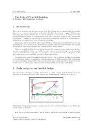
• CFD does not significantly reduce the cost of the actual design process, but it improves quality
and helps with the early detection of design flaws and this can lead to significant cost savings.
Within the first weeks of design, 40% to 60% of the total ship production cost is determined,
Johnson (1990). The costs of design modifications increase by orders of magnitudes
the further into the project they are made; ideally no fundamental modifications should be
made after the conceptual design phase. Achieving this goal can be greatly facilitated by the
use of CFD. If CFD is employed consistently to determine the final hull form at an earlier
stage, numerous decisions that influence the production costs can be made earlier in the design
process, thus reducing the risk of expensive design modifications being necessary later in
the project. This is especially important in the context of modern workflow methodologies
(e.g. concurrent engineering and lean production).
When assessing the economic benefits of CFD, merely considering cost aspects will therefore lead to
incorrect strategic decisions. We can assess the benefits of CAD by using an analogy with another
computer technology: CIM (Computer-Integrated Manufacturing), aptly put by Dietrich (1988):
“In other words, when taking CIM decisions, the question of ‘What will we save in
the short term?’ is not the right one to ask. The real issue is rather ‘How will our operational
situation develop if we do not introduce CIM?’ ”
3.2. Secondary Phase: Assessment and Decision
Areas suitable for the application of CAD (and / or CFD) may be selected considering:
24

• Departments / groups suited to CAD work; and
• Applications (products, processes).
An economic assessment should compare costs and benefits (benefits being savings and increased
turnover). Naturally, costs are easier to quantify than benefits. However, it is necessary (and possible)
to estimate most costs and savings to provide a sound basis for deciding on a CAD investment. Splitting
the total costs into individual items and estimating these items separately reduces the risk of gross
errors when estimating the total costs. Once costs and benefits have been (approximately) quantified,
a traditional assessment of the economic aspects (profitability) based on a dynamic method (discounted
cash flow) of the investment is trivial using a spreadsheet.
3.2.1. Costs Analysis
In introducing CAD systems, one should contemplate the following initial and running costs as detailed
below.
Initial costs:
• Purchase of hardware and software. (Leased software contributes to running costs.)
• Physical site installation (partitioning, furniture, lighting, air-conditioning, etc.)
• Hardware installation: cables, networks
• Software selection process (staff costs, travelling costs)
• Implementation
• Initial training, including opportunity costs due to loss of productive time
• Inferior performance (until the expected productivity gain is realized)
• Installation and integration of the software system (customised set-up, macros, interfaces)
• Data input: creation of fundamental databases and libraries
Running costs:
• Consumables, energy
• Maintenance and repair and updates to hardware that may be necessary to run the updated
software
• Software maintenance / updates
• Insurance
• Interest on bound capital
• Rental costs (rooms, data lines, hardware, software)
• Ongoing training, including opportunity costs due to lost productivity during training
• Staff cost (user and IT support staff)
• Data security and backup
Some of these costs may be negligible in which case they may then be omitted; this exhaustive list is
intended to prevent any cost items being overlooked.
3.2.2. Benefits Analysis
Now the more difficult task of estimating the benefits must be undertaken. Information on benefits
that might realistically be expected should not be based solely on the promises of software vendors,
although these may sometimes supply valuable information based on their experience with other customers.
The experience of other users within the same industry should be assessed and can be found
in publications, personal interviews and demonstrations. Software vendors may be able to help with
introductions to such users. Benchmark tests are useful to test individual systems under real conditions.
These tests should be selected by users to exercise the software’s capabilities using representative
examples of actual products and processes.
25

Users should quantify (and verify with the use of benchmark tests) the expected benefit that will be
provided by the software based on the following criteria:
• Modelling (for CAD: solid models, surface representation, hidden line removal, multiple view
techniques, maximum number of data structure elements, etc.; for CFD: grid techniques, grid
generation, turbulence modelling, cavitation modelling, free-surface technique, etc.)
• Programming (capability and user-friendliness of command language)
• Ergonomics (user-friendliness, GUI, help system)
• Additional applications for CAD systems (geometric and physical analyses, integrated NC
(numerical control) module, finite element analysis (FEA) pre- and post-processing, etc.)
• Display options (export of graphics, virtual reality models, videos, etc.)
• Interfaces for data exchange (STEP, IGES, VDA-FS, etc.; compatibility with common CFD
formats, e.g.: CCM+, Fluent, etc.)
While improvements in productivity due to implementation of a CAD system (in design, structural
design, production scheduling, assembly, etc.) may be estimated quite reliably, improvements in quality
and flexibility of workflow and capability are difficult to quantify. The following list gives some
items to contemplate in this context:
• Reduced time and costs for provision of existing products / services
• Potential for increased turnover due to ability to provide new products / services (due to the
extra capabilities of the software)
• Increased quality of products / services; reduced cost of quality control
• Improved product development (design)
• Greater level of detail available at concept design stage; e.g.: when bidding for tenders
There are various methods to quantify improvements in productivity for individual activities (e.g.
drawing or standard CFD analyses) that allow estimation of a PIF (productivity increase factor).
While the estimates for individual activities may have considerable error (or uncertainty), the average
PIF, obtained as the sum of all estimates, is usually accurate enough for the estimation purposes required
at this stage. The individual activities are weighted according to their frequency (time share) in
the usual operation of the company.
Further points in assessing the effect of CAD on profitability are listed below:
1. CAD improves product quality for constant capacity.
2. CAD improves productivity, i.e. unless staffing levels are reduced, CAD results in extended
capacity; if there is no corresponding increase in demand and staffing levels cannot or must
not be reduced, CAD investments will not pay off!
3. Flexible work hours increase CAD profitability.
For a better understanding of the cost of CFD use, it is useful to take a closer look at the workflow
pattern for CFD analyses:
1. Pre-processing (grid generation; specification of boundary and initial conditions; specification
of control parameters for the computation)
2. Computation
3. Post-processing (results interpretation; graphical output; report preparation)
These individual steps sometimes have to be performed repeatedly, in an iterative cycle. Cost aspects
will be discussed separately for each step:
26

1. Pre-processing:
Pre-processing requires staff that are familiar with specialist software for grid generation especially
on vessel hulls. This requires at least a basic understanding of the subsequent CFD
computations that will be performed. Grid generation is best performed on workstations or
fast personal computers. Time and labour costs of this step are mainly determined by the
user’s experience and the user-friendliness of the grid generation software. Pre-processing
represents the major part (40% to 80%) of the duration of most CFD projects. Staff training
and software (in-house development or licences) are the main fixed costs.
2. Computation:
The computation involves almost no man-hours except for computer supervision. State-ofthe-art
computations employ parallel computers. The fixed costs for these hardware architectures
are relatively small: for frequent (professional) users, typically less than 5% of total
costs.
3. Post-processing:
Post-processing involves production and interpretation of numerical, graphical and video output
from the CFD computations. The software required for the majority of post-processing
tasks is relatively inexpensive and often comes as part of an integrated CFD package. Highquality,
photo-realistic or interactive virtual-reality post-processing requires dedicated software
and user training, but their use remains, so far, the exception in maritime applications.
Post-processing also involves interpretation of results by experts and their documentation for
clients. User-friendliness of post-processing software and the use of standard graphical output
and report templates contribute to keeping time and cost requirements to a minimum.
4. The CFD Software Market from a Strategic Management Point of View
The CFD market is in a transitional phase from a young market to a mature market. The problems in
the pioneering days of CFD software can be attributed to the special features of highly-competitive,
immature markets as discussed, in a general way, by Porter (1980). These features can be summarised
as follows:
• Customer confusion due to contradicting statements from different providers
• Product reliability and quality problems
• Hesitant customers waiting for the next (cheaper and better) release
• Lack of standards and compatibility
• High fixed costs and low turnover for the providers, leading to high investment costs and insufficient
development power
Fortunately these problems have been largely overcome. A consolidation process has reduced the
number of serious suppliers to a point where stable conditions, benefiting the whole industry, appear
feasible.
However, there is always the opportunity for “new players” to arrive on the scene. This is particularly
true of universities who can often, relatively cheaply, develop new products (software modules) that
reflect the latest technologies and are often superior to existing software in terms of functionality.
However, if companies follow the guidelines suggested in this paper, especially if they consider strategic
and economic aspects, they will, almost always, decide in favour of established companies and
products. The high complexity of today’s software products and customer service requirements simply
do not favour “cowboy” software development companies. We may thus see a trend similar to the
aviation industry where, in the end, only a handful of companies will survive. In the long run, this
should be rather beneficial for the industry as a whole: fewer suppliers mean more customers per supplier,
i.e. more development power and the burden of development costs shared by more shoulders. It
27

also means that agreements on standards and data transfer between different products are easier to
achieve.
Recently, the open-source CFD package OpenFOAM, has attracted a lot of attention in the maritime
CFD community, Schmode and Bertram (2009). In the hands of well-trained users, OpenFOAM
yields good results for a variety of complex maritime flows (seakeeping with six degrees of freedom;
cavitating flows around propellers; sloshing with breaking waves; etc.), see e.g. the 2009 Numerical
Towing Tank Symposium, www.uni-due.de/imperia/md/content/ist/nutts_12_2009_cortona.pdf. Zero
licensing fees, wide scope of applicability and access to source code for personal modification and
research (that may lead to doctoral degrees) make OpenFOAM very attractive, particularly in the academic
environment. Industry users, on the other hand, should take a more prosaic perspective: savings
in license fees may be far less than the added costs of training. Experienced CFD users have reported
(in personal communication) that it took them several months to two years to come to terms with
OpenFOAM. Nevertheless, Germanischer Lloyd has decided to employ both commercial CFD software
(CCM+ developed by CD-adapco) and OpenFOAM in parallel. The investment of considerable
resources in a “free” software package was motivated by co-operative projects with several academic
partners. However, it is fair to say that the bulk of professional consulting work continues to be based
on the use of commercial software products.
5. Conclusions
A systematic approach to software selection is recommended. The outlined procedure is intended to
prevent important items from being overlooked. Specifically labour cost associated with training and
lack of productivity are frequently underestimated. Companies should select software based on how
long training will take and how much man-time will be required for a trained user to complete a typical
project. This in turn depends on user-friendliness, software user community networks, vendor support,
etc. For key software, strategic considerations are important to ensure long-term support by vendors.
For professional CFD applications, labour costs are decisive. Therefore vendors should focus on faster
(i.e. more automated) grid generation and post-processing.
References
BERTRAM, V. (1993), Economical aspects of computational fluid dynamics (CFD), 19 th WEGEMT
School, Nantes
BERTRAM, V.; COUSER, P. (2007), CFD possibilities and practice, The Naval Architect, September,
pp.137-147
BRUCE, G. (2009), Management information systems in ship repair, 8 th Conf. Computer and IT Applications
in the Maritime Industries (COMPIT), Budapest, pp.34-44
http://www.ssi.tu-harburg.de/doc/webseiten_dokumente/compit/dokumente/compit2009.pdf
COUSER, P. (2006), Selecting a suitable hull definition package, The Naval Architect, April, pp.42-
44; May pp.6-10; July/August pp.66-71
COUSER, P. (2007), Software for hydrostatic analysis of floating structures during their design, The
Naval Architect, January, pp.30-35; February, pp.71-75
DIETRICH, L. (1988), CIM Trends for the nineties, CIM-IT/Systems Conference, McKinsey & Co,
Berlin
FACH, K. (2006), Advanced simulation in the work of a modern classification society, 5 th Conf.
Computer and IT Applications in the Maritime Industries (COMPIT), Oegstgeest, pp.34-44
28

www.ssi.tu-harburg.de/doc/webseiten_dokumente/compit/dokumente/compit2006_oegstgeest.pdf
HOCHKIRCH, K.; BERTRAM, V. (2009), Slow Steaming Bulbous Bow Optimization for a Large
Containership, 8 th Conf. Computer and IT Applications in the Maritime Industries (COMPIT), Budapest,
pp.390-398
http://www.ssi.tu-harburg.de/doc/webseiten_dokumente/compit/dokumente/compit2009.pdf
JOHNSON, B. (1990), On the integration of CFD and CAD in ship design, Developments in Marine
Technology 6, CAD and CFD in Ship Design, Amsterdam
MENZEL, W.; EL MOCTAR, O.M.; MUMM, H. (2008), Advanced thinking on tricky excitations,
The Naval Architect, March, pp.64-69.
PORTER, M.E. (1980), Competitive strategy, MacMillan Publ.
SCHMODE, D.; BERTRAM, V. (2009), Wie OpenFOAM die CFD-Landschaft verändert, Hansa-
Journal, June
VDI (1990), Computer-aided design: Introducing strategies and economical benefits of CAD systems,
VDI Guideline 2216, Verband Deutscher Ingenieure
ZIEGLER, W.; FACH, K.; HOFFMEISTER, H., EL MOCTAR, O.M. (2006), Advanced analyses for
the EARTHRACE project, 5 th Conf. High-Performance Marine Vehicles (HIPER), Launceston,
pp.101-108
29

Optimisation of Single and Multi-Component Propulsors
Markus Druckenbrod, Jochen Hundemer, Moustafa Abdel-Maksoud, TU Hamburg-Harburg,
Hamburg/Germany, m.abdel-maksoud@tu-harburg.de
Max Steden, Howaldtswerke-Deutsche Werft GmbH (HDW), Kiel/Germany
Abstract
The paper describes the optimisation of a conventional propeller and a multi-component propulsor.
The last one can be used to satisfy high acoustic requirements. Both propulsors are optimised
concerning efficiency and cavitation behaviour for a ship with a given resistance at a ship speed of 20
knots. As thrust-fluctuations of a single blade can cause vibration and acoustic emissions, the
optimisation criteria is extended to include the minimisation of the amplitude of the unsteady blade
thrust force during one revolution in the investigated wake field.
1. Introduction
Modern ships require efficient propulsors with low sensitivity to cavitation within their operation
range. Up to a certain ship speed the mostly used propulsor is the conventional propeller which
reaches high efficiencies, but encounters cavitation problems at high speeds. One of the most common
propulsors for high ship speeds is the waterjet, with good performance characteristics at high speeds
on the one hand but with a significantly decreasing efficiency at low velocities on the other hand. Kim
(2006) shows typical propulsive efficiencies of the mentioned propulsors and also of super-cavitating
and surface-piercing propellers. The latter two propulsors are not treated here, as they are just feasible
for small ships.
Between the operational speed ranges of conventional propellers and waterjet propulsors there is a
field, where multi-component-propulsors appear to be advantageous. Such a propulsor, sometimes
also called pumpjet or linearjet, is called multi-component-propulsor in the present study. It consists
of the four components, Figs.1 and 2: rotor, hub, duct and stator.
Fig.1: Five-bladed multi-component propulsor
Fig.2: Seven-bladed multi-component propulsor
In a certain way, a multi-component-propulsor can be treated as a combination of a conventional
propeller and a waterjet. The water passes through the propulsor without being lifted to a higher level
as in the case of the waterjet. Therefore the theoretically attainable efficiency of a multi-component-
30

propulsor should be higher than that of a waterjet. The aim is to take advantage of having the duct to
achieve an increased pressure level at the rotor-position in order to avoid cavitation. Rising the
pressure level inside the propulsor, increases the risk of a raised rate of bypassing flow. In this case
the propulsor would not perform satisfactorily, as the mass flow rate would decrease and the intended
design point cannot be reached.
Compared to the conventional propeller, the duct reduces the strength of the tip vortex and the stator
helps to recover a part of the swirl energy from flow behind the rotor. These details provide good
prerequisites for the design of a high-performance propulsor. As the interactions among the single
components of the propulsor are quite complex, an appropriate technique has to be developed for the
design of such a propulsor.
Jürgens and Heinke (2006) carried out an experimental and numerical investigation to study the effect
of the design variables on the performance of the propulsor. The results show that a variation of the
rotor’s pitch-ratio and the hub-diameter influences the hydrodynamic properties strongly, whereas the
blade-number has a secondary effect. Cavitation occurs primarily at the gap between the inside wall
of the duct and the rotor blade’s tip.
A design procedure for waterjet propulors was described by Kerwin (2006). The paper describes a
potential theory based solver with the consideration of the inhomogeneous wake field entering the
duct. The influence of the duct on the flow field around the rotor and the stator is considered by
coupling the potential flow solver with an Euler code. The forces of rotor and stator are transferred to
the Euler solver to simulate the effect of the accelerated flow inside the duct due to the generated
thrust. A similar body-force model was included in the RANSE simulations performed here.
2. Optimisation Algorithms
Two different evolutionary algorithms are used in this study. Evolutionary algorithms apply the
principle of the biological evolutionary process to mathematical problems. The optimiser generates
several sets of parameters, where each set describes a propulsor design. Each design is called
individual, with its chromosomes, the parameters. Evolutionary algorithms typically create several
individuals at once, which have to be evaluated afterwards. Such a group of individuals, each
individual standing for a certain propulsor design, is called a generation. After the designs of a
generation have been evaluated, the best are selected; the chromosomes of the selected individuals are
exchanged and slightly varied to prevent stagnation. With these three steps - selection, recombination
and mutation - the fittest individuals survive and better individuals should be generated.
The evaluation of an individual means that the performance of a design has to be calculated and its
quality regarding an objective function has to be evaluated. An objective function, which has to be
defined by the designer, expresses all important design criterions and should reach a minimum value
for the optimal desired propulsor. A better design will obtain a smaller value, and hence it will be
preferred during the selection. Besides the single objective optimisation, where all design criterions
are integrated into one objective function, some optimisation algorithms use multi-objective
optimisation, where dependencies between design criterions can be identified.
The first optimisation algorithm used in the present study is the NSGAII (Non-dominated Sorting
Algorithm). It is able to optimise multi-objective problems and can be applied in single and multi
objective mode. In the present study, 20 generations are considered with eight individuals each.
The second algorithm applied in this study is the MAEA (Metamodel Assisted Evolutionary
Algorithm). It solves single objective problems. Meta-model is a general function defined in the
optimisation algorithm, which allows an estimation of the fitness of an individual, without calculating
the hydrodynamic performance explicitly. The meta-model is based on the results calculated during
the optimisation and relates the parameters of the evaluated individuals to the corresponding value of
the objective function. Only those individuals with a promising result in the meta-model are evaluated
31

with the more precise flow solver. This strategy aims to minimize the number of time consuming flow
calculations. The Meta-model Assisted Evolutionary Algorithm was developed at the Department of
Computer Science, Chair of Algorithm Engineering TU Dortmund. The integration of the MAEA
optimisation algorithm into a propulsor optimisation process is described by Hundemer et al. (2006).
3. Flow Solvers
Two different solvers are used in the present study. In all optimisation processes the in-house
potential theory solver ISThydro is included, which is a first-order 3D- panel method. The ISThydro
solver represents the propulsor by a distribution of constant strength sources and dipoles on the
panelised geometry. The strength of the sources and dipoles are to be determined during the
calculation. The method can be applied to simulate steady or unsteady flow problems.
The used RANSE solver is the commercial code ANSYS-CFX, www.ansys.com. It is utilised to
optimise the duct geometry and the hub of the propulsor. The SST-turbulence model is applied and a
hexahedral mesh is employed for the viscous flow calculations in the study.
4. Optimisation Process
The optimisation starts with the generation of a set of design variables. Then this set is used to create
the first geometry and a mesh for the numerical computation. The mesh is passed to the solver, which
simulates the flow generated by the propulsor which finally leads to its hydrodynamic performance.
The calculated performance data is used to estimate the objective function. For an automatic
optimisation of a propulsor geometry, all these steps are combined in one optimisation process.
For a successful realisation of an optimisation process the geometry of the propulsor has to be
described by an appropriate parametric model, which does not necessarily follow the common
description of a propeller blade in cylinder coordinates. Such a parametric model is only valid in a
certain range, in which the parameters may vary during the optimisation. This range has to be defined
before starting the optimisation. The number of design variables should be kept as small as possible;
otherwise the optimisation algorithm will not be able to handle the large number of design variables
efficiently. Furthermore an appropriate objective function has to be defined, which represents the
optimisation targets in a satisfactory way.
The propeller blade is parameterized according to Hundemer et al. (2006). This can be summarised
for the case of chord length as follows: The radial chord distribution can be considered as a product of
two functions and a factor, which allows adjusting the blade area to a desired aspect ratio.
f
r r r
( ) = f1( ) ⋅ f
2
( ) ⋅ c1
R
R
R
f 1 is a square root function, which describes the general shape of the blade. The square root enables a
round tip with a chord length reducing to zero at the tip. f 2 is a spline curve defined by its values at
hub and tip and the derivation at both points. While the value of the function at the hub is set to 1, the
three other values are considered as parameters. Factor c 1 scales the function so that a desired
expanded blade area ratio is obtained. The radial pitch distribution is generated in a similar way. The
pitch is defined by the product of a factor c 2 and B-spline curve g 1 . The points defining the spline
curve are related to each other, so that a typical pitch distribution with an unloaded tip and a reduced
hub loading is achieved.
g
r
r
( ) = g 1
( ) ⋅ c2
R
R
Factor c 2 scales the pitch distribution to obtain a desired pitch at the relative radius r/R = 0.7.
The propeller geometry is modified by varying the radial distribution of the chord length and the pitch
while the propeller diameter, number of blades, number of revolution and skew are fixed. The profile
geometry is kept also constant. The investigated propeller in this study is a seven bladed one.
32

The FRIENDSHIP Framework software developed by FRIENDSHIP Systems GmbH is applied for
the propeller optimisation, www.friendship-systems.com. The geometry description of the propeller
and its mesh are modelled parametrically within the FRIENDSHIP Framework, which also controls
the optimisation algorithm. For the propeller optimisation the implemented NSGAII algorithm is
used. In the present study two different propeller optimisation runs are realised. During the first
propeller optimisation the objective function consists of three sub-functions. The aim of the first one
is to achieve a targeted thrust, the second and the third are used to minimise cavitation and to
maximise the efficiency. During the second run the multi-objective optimisation algorithm NSGAII is
applied. An additional second objective function is defined to minimise the thrust amplitude of a
single blade axial force during one rotation.
For the optimisation of the multi-component-propulsor MAEA algorithm is applied. An overview of
the total optimisation process is given in Steden et al. (2009). Geometry and mesh are generated by an
in-house CAD routine. The propulsor geometry is varied by changing the parameters of all four
components hub, duct rotor and stator. The geometry of rotor and stator blades and duct are varied by
changing their camber line. The duct geometry in addition is changed by modifying the thickness
ratio. The objective function of the multi-component-propulsor optimisation is defined in such a way,
that a certain thrust has to be achieved, cavitation is minimised and efficiency is maximised.
Four propulsor geometries were developed for the same operation condition during the present study,
two propellers and two multi-component-propulsors. To investigate the influence of the number of
rotor blades on the unsteady behaviour of the thrust force of multi-component-propulsors, two rotor
geometries were developed, one with five and one with seven blades. The number of stator blades is
six for both. The rotor and the stator blades are surrounded by the duct and fixed to the hub. The
design was optimised in two steps. In the first step the duct geometry was optimised under
consideration of a constant radial thrust distribution in the rotor plane with the help of the RANSE
solver. In the second step, the rotor and stator were optimised by means of the potential flow code for
a fixed duct and hub geometry. For both steps the MAEA optimisation algorithm was used. To
evaluate the calculated unsteady thrust behaviour of a single blade and the propulsor a frequency
analyse was applied.
5. Results
The estimation of the unsteady behaviour of the propellers in the ship wake requires that all blades are
modelled in the numerical calculation. In this case the number of the applied panels is equal to the
number of panels per blade times the number of blades, as a periodic boundary condition cannot be
applied. The computation time can be reduced significantly, if only one blade is resolved with a fine
grid, while a coarse grid is applied to the other propeller blades. The blade with the fine grid
resolution is used to calculate the forces acting on the blade. For consideration of the interaction with
other blades, the accuracy of the applied coarse grid results is sufficient for the aim of the study.
Table 1: Influence of the numerical grid on the calculated thrust
Fine grid:
Coarse grid:
Results:
Configuration I Configuration II Configuration
III
u-direction: 20 20 20
v-direction: 17 17 17
u-direction: 20 17 15
v-direction: 17 15 15
Thrust: 100 99.94% 100.72%
Thrust difference: -0.06% 0.72%
Calculation Time: 48 min 41 min 29 min
33

Before the beginning of the propeller optimisation a grid sensitivity study was made to analyse the
influence of the different grid strategies on the results. So the thrust coefficient was calculated for a
propeller geometry with three different grid configurations. The calculated results and applied grid
resolutions are presented in Table 1. Due to the considerable reduction of calculation time (about 40
%) and the limited influence on the accuracy of the estimated thrust (less than 1%), grid configuration
III was selected for the further calculations.
Fig.3: Propeller design “Optim I”
Fig.4: Propeller design “Optim II”
The optimised propeller geometries I and II are shown in Figs.3 and 4. Propeller I is optimised by
employing a single criterion target function without taking into account the minimisation of the thrust
amplitude of a single propeller blade. This additional criterion is considered during the optimisation of
propeller II. In both cases the NSGAII optimisation algorithm is used.
Fig.5: Radial distribution of pitch ratio
Fig.6: Radial distribution of chord length ratio
Table 2: Comparison of two propeller designs
Propeller “Optim I” Propeller “Optim II”
Cavitation: 0.40 % 1.80 %
Efficiency: 66.3 % 63.6 %
Amplitude / Target Thrust: 35.6 % 31.6 %
The calculated radial pitch and chord length for the two propellers are shown in Figs.5 and 6. While
propeller I has a relatively high blade area and a low pitch, the propeller II shows the vice versa
34

ehaviour for both parameters. Table 2 includes the efficiency, the amplitude of blade thrust
fluctuation and the calculated cavitation area, where pressure on the blade is lower than vapour
pressure. The cavitation area is given in percent of the total blade area.
The comparison of the both designs shows that the reduction of thrust fluctuation can be achieved by
increasing the pitch angle. The thrust fluctuation is a result of the variation of the inflow angle due to
the three-dimensional wake field. A high pitch angle of the blade reduces the effect of the inflow
angle fluctuation on the total angle of attack of the profile. The smaller blade area leads to higher
loaded blades, as thrust remains the same for both designs. The high induced velocities by the
propeller blades of the second design will reduce the influence of the fluctuation component of the
inflow velocity on the total angle of attack of the profile. Therefore a reduction of the amplitude of
blade thrust fluctuation should be expected. This advantage is achieved on the cost of cavitation
behaviour and efficiency, see Table 2. The calculated hydrodynamic performance of both geometries
is shown also in Fig.7.
Fig.7: Performance characteristics of the optimised propellers
The first optimised multi-component-propulsor geometry has a five-bladed rotor, which is shown in
Fig.1. The main parameters affecting the geometry of the duct are flow rate and mean radial
circulation distribution in the rotor domain. Since both multi-component-propulsor geometries are
developed for the same operating point, the parameters for the duct design are identical. That allows
the use of one optimised duct geometry for two rotors. Figs.8 and 9 show the mean radial thrust
distribution in the rotor domain and the developed duct geometry.
Fig.8: Mean radial distribution of rotor circulation
Fig.9: Duct and hub geometry
There are many requirements to be met during the duct optimisation. Flow separation on the leading
edge of the duct must be avoided and the ratio between the inlet and outlet area has to be achieved.
The increase of the pressure level in the rotor domain leads automatically to an increase of the duct
resistance, Fig.10. Each point in the figure shows the resistance of the duct geometry in percent of the
total thrust and the corresponding pressure level inside the rotor domain. The calculated results show
35

that high pressure level in the rotor domain is coupled with high duct resistance. Therefore based on
the aim of the design it is important to achieve an acceptable compromise between the duct resistance
and pressure level in the rotor domain. In the presented case the resistance of the selected duct is less
than 0.5% of the total thrust.
Fig.10: Relation between duct resistance and pressure increase in rotor domain
A comparison of the radial distribution of pitch ratio and chord length ratio for both designs is given
in Figs.11 and 12. The propulsor with the five-bladed rotor shows a higher pitch distribution on
almost radii range, while for the chord length the situation is contrary. The thrust oscillation for the
considered wake field over 360° is calculated by quasi-steady technique. Similar numerical
investigations show that quasi-steady computations overestimate the thrust oscillation in comparison
to unsteady ones. However the quality of the quasi-steady results is adequate to compare two designs.
Fig.11: Radial distribution of pitch ratio for the
optimised multi-component propulsors
Fig.12: Radial distribution of chord length ratio
for the optimised multi-component propulsors
Fig.13 represents the thrust oscillation for a single rotor blade. The calculated results are normalised
by the averaged thrust of one rotor blade. The oscillation of the total thrust is estimated by superpositioning
the thrust of all rotor blades under considering the relative angular positions between the
propeller blades, Fig.14. The target thrust is used to normalise the data. The comparison of the results
in Figs.13 and 14 shows the similar tendency as in the propeller optimisation. The thrust oscillation of
one rotor blade can be reduced by increasing the pitch. As expected, in the case of considering all
rotor blades, the oscillation of the total thrust with the high number of blades is lower.
The results of the frequency analysis of both designs are included in Figs.15 and 16. The analysis is
carried out by applying Fourier transformation technique. The results of single rotor blade show that
the dominating orders are the first and the third one, Fig.15. Considering all rotor blades, the fivebladed
design shows significantly higher amplitudes of the first order. Another advantage of the
design with the seven-bladed rotor is the higher efficiency in comparison to the five-bladed
configuration, see Table 3 and the open-water performance characteristics in Fig.17.
36

Fig.13: Thrust oscillation for single rotor blade
for the optimised multi-component propulsors
Fig.14: Thrust oscillation for all rotor blades
for the optimised multi-component propulsors
Fig.15: Frequency analysis for the thrust force
of single rotor blade
Fig.16: Frequency analysis for the total thrust
force of the rotor blades
Fig.17: Performance characteristics of the optimised multi-component propulsors
Table 3: Comparison of two multi-component-propulsor designs
Multi-Comp. I Multi-Comp. II
Cavitation: 0.39 % 0.0 %
Efficiency: 68.6 % 73.6 %
37

6. Conclusion
In comparison to a conventional propeller the design of a multi-component-propulsor is more
sophisticated. The application of modern optimisation methods is necessary to achieve a design,
which is able to fulfil the most important design requirements.
The drawback of applying optimisation methods is the over-proportional increase of computation
effort. Due to the high number of design variables of a multi-component-propulsor, a huge quantity of
designs has to be created in order to estimate the influence of design parameters on the performance
of the developed geometries. Therefore it is important to combine the advantages of calculation
methods for potential and for viscous flow to reduce the computation time and accelerate the
optimisation.
From the hydrodynamic point of view multi-component propulsors are more efficient than propellers
at a certain ship speed range and for certain applications. The employing of the duct can be helpful
also for ships working in extremely shallow water because the duct protects the propeller in grounding
case. Another important advantage of the employing of the duct is the expected reduction of the
hydro-acoustic impact on the environment. The expected high manufacturing costs make multicomponent
propulsors for conventional commercial applications too expensive.
References
HUNDEMER, J.; NAUJOKS, B.; HACHMANN, T.; ABDEL-MAKSOUD, M. (2006), Design of
ship propellers with evolution algorithms, Jahrbuch der STG, Springer
JÜRGENS, D.; HEINKE, H.J. (2006), Investigation of deeply submerged waterjet, Jahrbuch der STG,
Springer
KERWIN, J.E. (2006), Hydrodynamic issues in waterjet design and analysis, 26 th
Hydrodynamics, Rome
Symp. Naval
KIM, K.H. (2006), Waterjet propulsion for high-speed naval ships, Advanced Naval Propulsion
Symp., Arlington
STEDEN, M.; HUNDEMER, J.; ABDEL-MAKSOUD, M. (2009), Optimisation of a linearjet, 1 st Int.
Symp. Marine Propulsors, Trondheim
38

Training Complex for Training Submarine Motion Control Skills on the
Basis of Virtual Dynamic Systems
Valery Mrykin, Vyacheslav Lomov, Sergey Kurnosov,
Central Design Bureau for Marine Engineering "Rubin", St.Petersburg/Russia, neptun@ckb-rubin.ru
Manucher Dorri, V.A. Trapeznikov Institute of Control Sciences of the Russian Academy of
Sciences, Moscow/Russia, dorrimax@ipu.rssi.ru
Abstract
Problems arising during development of training aids for training submarine crews in training
centres are considered in the first part of the presentation. Results of development work for tools and
computer-aided technologies are covered in the second part. They make it possible to display in
interactive manner the submarine control systems that were used for the development of the training
facility to exercise tasks for control of modern submarine motion systems and optimization of control
algorithms. This training facility may be used for both individual training of operators of submarine
motion control in training centres and for optimization of control algorithms in design engineering
firms.
1. Introduction
Navy has been using instructional/training aids for training of submarine crews. These aids ensure an
adequate training both of single specialists and the entire crew. Many enterprises such as design
bureaus, research institutes, instrument-making research-and-production concerns and training centres
are usually involved in the accomplishment of this challenging task.
The main line of activities in this field consists in making by the above-mentioned enterprises of
information/technical training aids represented by special-purpose and multi-purpose training
facilities. Thereafter these products are supplied to the Navy Training Centre to be used for training of
submarine crews. Officer personnel, junior officers and seamen being in service on a contract basis
are enabled to get practical skills in maintaining the technical facilities in normal conditions of
operation and in case of emergencies. The important activity includes works on mastering of modern
computer technologies which are promising for further development and improvement of
instructional/practical training aids for submarine crews. Computer technologies make it possible to
represent the information about the submarine dynamic state in visual pictorial form that is required
for high-quality training of the crew.
2. Aids for training of submarine crews
Real consoles of submarine and submarine technical facilities control (including front panels of
consoles of automatic motion control systems, monitors with video frames, repeaters and tableau
buttons, keyboards, etc. connected to simulators of signals generated by various systems on the basis
of mathematical modelling) are normally used for training of submarine crews at Training Centres. In
some cases, facilities used for displaying the information about a submarine and elements of control
systems are complicated systems consisting of computers, monitors and signal simulators clustered in
a local network.
The console of submarine motion control system is shown in Fig.1. The control from the console
shown in Fig.1 and similar consoles is performed both by using physical controls and virtual controls,
one or another type of control being displayed in video frames similar to the one shown in Fig.2.
39

Fig.1: Console of Submarine Motion Control System
Fig.2: Video Frame Displayed on Console of Submarine Motion Control System
3. Basic Principles of Training Complex for Training Submarine Motion Control Skills
3.1 Work of Operators of Submarine Control Systems
Submarine operators have to work in difficult conditions characterized by insufficient information
support, action of extreme factors, tight limitations on time for taking of decisions. E.g., the operators
are forced to assess the surrounding situation based on instrument readings and technical system
indications. In some cases, the complexity of tasks to be performed, large scope of incoming data and
insufficient time for taking decisions result in failure of a human operator being a “decisive element”
in the decision-taking loop (since it is the operator who implements the algorithm of the on-line
search for control decisions) to meet the requirements for efficient process of the on-line control of
submarine motion and technical facilities operation. This situation leads to decrease in control
efficiency and does not ensure an appropriate safety level as illustrated by actual submarine accidents.
Therefore increased information support for operators of submarine manoeuvring control systems
remains an important issue as more advanced control systems are being developed.
3.2 Virtual Dynamic Systems
With the appearance of new computer facilities and technologies, the representation of information
about the state and position of submarine control systems by using virtual dynamic systems became a
40

feasible option to improve the training of operators of motion control systems. Virtual dynamic
systems enable an integral representation of minimum information required for performing a specific
task in pictorial and easy-to-understand form. They simulate input for human senses similar to those
felt in reality or visualize information about ongoing processes.
The possibility to study the behaviour of one or another object by using the pictorial representation of
object and environment where the processes take place in the clearest and most realistic form is an
essential advantage of virtual dynamic systems. Three-dimensional representation and software tools
allow the simulation of the surrounding situation in dynamics from different viewpoints of observer
play an important role. The virtual dynamic systems allow keeping likeness of simulated processes to
real processes taking place onboard an object and represent these processes within specified spatial
and time limits. This property is essential for successful training in control, prediction of complex
emergencies, development of intuition as well as for design and improvement of systems being newly
developed.
The virtual dynamic systems created by means of tools available now are dedicated software products
of high cost and insufficient versatility. They cannot be used for similar objects without significant
modifications by highly qualified software engineers. Special tools will allow creating virtual
dynamic systems in short time and at minimum expenses for systems representing the information of
various purposes including research simulators for submarines.
Therefore when creating the training complex on the basis of virtual dynamic systems, the task was to
develop scientific/methodological fundamentals for making tools for interactive construction of
virtual dynamic systems. A block-hierarchical structure would reduce time and cost of developing
full-scale training facilities for virtual submarine prototypes. Blocks contain computing algorithms for
pictorial representation of the submarine state and the surrounding situation.
3.3 Software Package for Dynamic System Calculation
At present, based on the results of joint activities of V.A. Trapeznikov Institute of Control Sciences,
CDB ME “Rubin” and “Avrora” Corporation Science & Production” has developed a training
complex for submarine manoeuvring control with visualization elements of environment on the basis
of virtual dynamic systems. The training complex shown in Fig.3 was exhibited at the International
Maritime Defence Show in St. Petersburg in 2009 and aroused interest among specialists.
Fig.3: Training Complex of Manoeuvring Control System
The proposed training complex is based on the software tool package developed by the Institute of
Control Sciences named after V.A.Trapeznikov (Dynamic System Calculation), Dorri et al. (2006). In
the course of creation of the package, its overall structure which consists of a shell executive program
(development environment) and set of block-modules performing different tasks has been determined.
41

The type and composition of modules in use depend on the purpose of virtual dynamic system under
development and customer’s requirements. As a result of module construction analysis, the data
structure of all-purpose block of the system and data structure of sub-systems were determined. The
form and type of data flow transmitted through links were selected. The necessity for conditions to be
created for automatic compilation of executive programs of blocks was shown.
The arrangement principles of software tool package for calculation of dynamic systems have been
addressed including such aspects as:
1. Modes of package operation and general principle of virtual dynamic system calculation
2. Data transmission through buses
3. Vector images of blocks
4. Control of blocks and links actuation
5. Split of structure into layers
6. Group assignment and setting of block parameters
7. Running of package on several computers
8. Interaction of package with other programs
9. Connection with real equipment
Fig.4 shows fragments of operator’s virtual station for manoeuvring control system made by using the
software package of dynamic system calculation. The screen displays the video frames pertaining to
the control of the operator consoles for submarine planes and rudders. These in turn control the
submarine motion. In the left part of the video frame, the usual representation of the submarine course
is kept in the form of rotating compass card with rough and fine readings. The information about rate
of course change is displayed additionally. The submarine position in space with respect to list is
displayed in dynamics as a submarine cross section in the upper left part of the video frame. The
submarine position with respect to depth and trim is displayed in the right part of the video frame. The
submarine image moves vertically along the depth scale and concurrently changes its angle of
inclination depending on trim. When the submarine enters the depth stabilization zone, the precision
scale is displayed. For displaying accurate current and specified values of all parameters, there is a
common panel in the upper right part of the video frame. The same panel is used for entering the
specified values. Using the keyboard, one can get to the line “SPECIFIED” and thereafter select a
desired parameter to be changed.
Fig.4: Video Frames of Training Complex of Manoeuvring Control System,
Left: Main Video Frame, Right: Additional Video Frame
Limitations on parameters of submarine motion and angles of control surfaces are changed in a
similar way.
42

In addition, the submarine’s animated three-dimensional image is shown in Fig.5. The motion
parameters of this image relative to imagined sea and bottom surfaces as well as the imagined centre
of gravity are changing in compliance with those controlling actions by controls that are set using the
video frame of the manoeuvring control system and master video frame shown in Fig.4 and Fig.7
respectively.
Fig.5: Representation of Spatial Motion, Left: Main Video Frame, Right: Additional Video Frame
Fig.6: Representation of Spatial Motion in Surface position, Additional Video Frame
The video frame shown in Fig.5 is meant for representation of the submarine state. This video frame
contains minimum required, but still sufficiently full information about control facilities and
submarine state in space. The power is given to the operator to assess the situation using the threedimensional
image shown in Fig.5 and refine the values of motion parameters by scale instruments.
Fig.7 shows fragments of the master video frame for setting the submarine motion control algorithms.
Fig.7: Fragment of Master Video Frame
Fig.7 shows the submarine main controls – control surfaces, tanks and propulsor (screw propeller). By
using these controls and setting the control actions in the subsystem, the tasks of submarine control
can be performed both in operating and special navigation conditions and also in emergency
conditions (jamming of control surfaces, flooding of pressure hull compartments, mistakes made by
control system operator, etc.). Parameter indicators are specially zeroed. The images of all equipment
43

units are animated by using tools of the software package. A change in position of control surfaces,
water levels in tanks, air pressure in bottles, opening and closing of valves and kingstons are
represented in sketch form. In addition, vectors of forces acting on a submarine are shown
symbolically and various numerical indicators are displayed.
Of course it is possible to turn off some screens after explanation of the essence of ongoing events,
keeping in operation only those screens that are available onboard a submarine and then practise
actions of operators when the information about submarine equipment units and gears is incomplete.
Any wrong actions of operators can be analyzed later using more thorough simulation screens. Such
training will contribute to intelligent actions of crew members in difficult control conditions and
emergency situations without hampering exercises with full-scale training facilities.
A full-scale training facility could include subsystems shown in Fig.3 to 5. They would represent
processes of submarine motion on a set of monitors from the point of view being of interest for
different specialists, Dorri et al. (2007). Using the training facility, it would be possible to enter
various control and disturbance actions and observe processes in progress. Ideally, the training facility
could have synthesizing and optimizing algorithms of automatic control theory in its arsenal.
For an operator, a simulated system looks like a structural diagram where links between blocks are
represented graphically in the form of lines. The external view of blocks can vary in the process of
simulation, making the information about the results of calculation and system state more
demonstrative for the user. The results of calculation can be generated in the form of numbers, graphs,
indicators, etc. In addition, the user can intervene in the system operation directly during the
simulation by changing parameters of blocks and observing the results caused by these changes. The
whole system of dynamic system calculation is constructed under Windows environment using
C++Builder and employs service facilities that are comfortable for majority of users.
The visualization of the process of tank blowing-out and changes in compressed gas weight in bottles
is developed within the software package in the visualization module of tank flooding/blowing
dynamics. Values of pressure in tank and bottle, outboard pressure and water volume in tank are
displayed on indicators. Processes of water intake to and discharge from the tank are represented on
graphs.
Non-linear characteristics of different modules of the training complex are specified in the form of
piecewise linear functions. Standard program modules have been developed for the purpose of
specification of non-linear characteristics of controlled object and control facilities. Employing the
matrix-editing block which output is connected to the interpolation block input the user enters a
matrix that contains coordinates of piecewise linear function points.
Employing the specialized software product OpenGL the submarine three-dimensional motion has
been simulated in the subsystems which simulate submarine three-dimensional motion. The forms
have been developed using which dimensions, colours and other characteristics of submarine threedimensional
motion can be selected. These forms make it possible to vary and refine the data in the
interactive mode and demonstrate the result on the monitor screen.
The software package is able to simulate systems represented in the form of a set of interconnected
modules each of which can contain the calculation program that determines the interaction with other
system modules and response to user actions. The groups of functionally related blocks can be
combined in composite blocks (subsystems) which can contain their own program in addition to those
contained within the subsystem of blocks. An example of visualization of such a module for control of
aft planes is shown in Fig.8.
All programs of blocks are loaded from external libraries that can be modified independently of
master program.
44

Fig.8: Visualization of Operation of Plane Control Module
The main advantages of the software package are as follows, Dorri et al. (2005):
1. It is possible to provide a simple and demonstrative image representation of each system
block.
2. A wide range of types of information transfer between blocks is acceptable when making
models.
3. A provision is made in the package to create models and their interfaces at different visibility
layers.
4. The package admits a hierarchical structure of blocks and use of complex modules on a par
with simple modules.
5. The package allows specifying the logics of operation of blocks and thus simulating any
logically constructed system like algorithm block diagrams and Petri nets.
6. The package has facilities to control the process and intervene in progress of the dynamic
process directly from the monitor screen.
7. It is allowed that auto compilation blocks are created by designers of control systems.
8. There are facilities for visualization of control processes and behaviour of controlled objects.
9. It is possible to solve problems using fast-time scale and in real time that facilitates the use of
the package for constructing the package links with real equipment of submarines.
10. It is possible to develop and check the algorithms and software for modern control systems of
submarines working with real facilities in conditions of pseudo full-scale simulation.
11. It is possible to apply modern methods of control theory to development and improvement of
submarine motion control systems.
12. It is possible to provide the virtual development environment for operators where the effects
caused by one or another disturbance and failure in operation of equipment are clearly
demonstrated.
4. Field of Application of Training Complex
The training complex can be used for optimization of control task at design institutions. The
experience of working with the complex gained at CDB ME “Rubin” in the process of optimization of
submarine control tasks and writing of control instructions has shown that the simulator is efficient
when it is used for development and evaluation of algorithms of submarine motion control in different
motion modes. Usually before developing the control instructions the optimization of submarine
control is being carried out using the simulation systems that make possible the quantitative and
45

qualitative evaluation of successful performance of submarine control tasks in various conditions for
different modes. However the visual presentation of submarine control systems is not available. This
is feasible only onboard a submarine or at Training Centres. The employment of the suggested
training complex makes it possible to reject expensive and large-size equipment of full-scale training
facilities used in training centres.
Also the training complex can be used for individual preliminary training of operators of submarine
motion control consoles before they start their training at Training Centres. At the same time the
employment of the training complex as a facility of preliminary training of operators does not
depreciate the importance of training at Training Centres. Quite on the contrary, such a way allows
acquiring skills in control of submarine technical facilities faster. There is no doubt that final skills in
motion control are to be mastered at Navy Training Centres using real consoles that simulate working
places of operators of submarine control systems. Nevertheless, the training complex considerably
reduces the duration of operator training and improves the quality of training because it helps trainees
in deeper understanding of submarine control processes. The training complex is developed for
manoeuvring control system of a specific submarine. It is possible to make a similar simulator which
simulates the operation of control system of submarine technical facilities and is intended for
optimization of control of submarine technical facilities, e.g. in the process of submarine diving and
surfacing. On such a training complex (like on a real control console) it is possible to perform
operations, e.g. blowing and flooding of tanks, and master the modes of submarine diving and
surfacing. The training complex can also be employed when adjusting separate training tasks for fullscale
training facilities at Training Centres, including the verification of mathematical models of
submarine behaviour and operation of technical facilities in the course of delivery/acceptance of large
training complexes intended for training of submarine crews. Besides, the training complex is
essential for a rapid analysis of field tests which is to be conducted directly onboard the submarine
and concerns the results obtained in the course of acceptance tests both of a submarine proper and
various systems fitted onboard.
5. Conclusions
The training complex which can be constructed using the software package of dynamic system
calculation for a maximum possible number of submarine control systems would be very useful for
developing the skills of submarine personnel in control of submarine technical facilities.
An essential difference of the training complex designed for optimization of tasks of modern
submarine motion control and operation of submarine technical facilities from fixed training
equipment is its compact size and easy use. The training complex requires neither complicated
hardware (computer system, special rooms, etc.) nor skills in programming to make some kind of
changes and additions to the training complex software.
The training complex not only facilitates the writing of submarine operating instructions in effective
and proper manner, but it can also be an interlink between a design institution and training centre
because the real processes being represented correctly but in a simplified form will help to cope with
operation of full-scale training complexes at training centres.
Modern visualization facilities make it possible to develop virtual dynamic systems which simulate
on-going processes and thus clearly explain the effects caused by one or another action of operators
dealing with the submarine control.
The illustrative images of consoles and training complex included in this paper give an idea about
search for and advancement of ways of information representation in dynamics used for evaluation of
operation of control facilities and submarine state in space.
46

References
DORRI, M.K.; KORCHANOV, V.M.; OSTRETSOV, G.E.; POPOV, P.V.; ROSHCHIN, A.A.
(2005), Advancement of systems representing information about control facilities and submarine state
in space, Collected Papers of XXXII All-Russia Conference on Sea Vessel and Special Vehicle
Motion Control, Moscow, pp.9-16
DORRI, M.K.; KORCHANOV, V.M.; OSTRETSOV, G.E.; ROSHCHIN, A.A. (2006), Principles of
development of full-scale research simulators and ways of their implementation based on software
package “Dynamic System Calculation”, Collected Papers of XXXIII All-Russia Conference on Sea
Vessel and Special Vehicle Motion Control, Moscow, pp.28-36
DORRI, M.K.; ROSHCHIN, A.A. (2007). Organization of interaction and data exchange between
several computers on stand designed for studying algorithms of submarine motion control, Collected
Papers of XXXIV All-Russia Conference on Sea Vessel and Special Vehicle Motion Control,
Moscow, pp.15-19
47

Ship Structural Optimization under Uncertainty
Jose Marcio Vasconcellos, COPPE/UFRJ, Rio de Janeiro/Brazil, jmarcio@ufrj.br
Abstract
This article discusses the application of Genetic Algorithms to ship structural optimization and the
treatment of variables with a degree of uncertainty. The variable uncertainty is included in the
simulation using a Monte Carlo approach. The software ModeFrontier TM is applied in the case study
for a double-hull tanker midship section design.
1. Introduction
Optimization problems are problems in which one seeks to minimize or maximize a real-valued
objective function by systematically choosing the values of real or integer variables from within an
allowed set, which may be subject to constraints. Many real problems present uncertainty in their
variables: They are inherent to the majority of physical, chemical, biological, geographical systems,
etc. Stochastic optimization methods are optimization algorithms which incorporate probabilistic
(random) elements, either in the problem data (the objective function, the constraints, etc.), or in the
algorithm itself (through random parameter values, random choices, etc.), or in both. The concept
contrasts with the deterministic optimization methods, where the values of the objective function are
assumed to be exact, and the computation is completely determined by the values sampled so far.
There are many stochastic optimization techniques. We will use here Genetic Algorithms (GAs) and
Monte Carlo simulation.
Our objective is to minimize the section area of a double-hull tanker ship as a measure of weight. We
use classification society based rules and investigate the possibility of uncertainty in some plate
thickness. The main origin of the uncertainty could be the shipbuilding process and the corrosion
behavior.
2. Methodology
2.1. Genetic algorithms
Genetic Algorithms are adaptive heuristic search algorithms built on the idea of genetics, natural
selection and evolution. The basic concept of GAs is designed to simulate processes in natural system
necessary for evolution, specifically those that follow the principles of survival of the fittest. As such
they represent an intelligent exploitation of a random search within a defined search space to solve a
problem.
The selective mechanisms carry out the changes that determine the evolution of a population over the
generations. Such changes can occur due to the interactions between the individuals or due to the
influence of the environment on the individual. Three basic mechanisms derive from this: crossover,
reproduction and mutation. They are called genetic operators and are responsible for carrying out the
evolution of the algorithm. The application of these operators is preceded by a selection process of the
best adapted individuals, which uses a function called the fitness function (a.k.a. adaptation function).
An implementation of a genetic algorithm begins with a random population of chromosomes, i.e. the
initial population can be obtained by choosing a value for the parameters or variables of each
chromosome randomly between its minimum and maximum value. Then each individual is evaluated
through the objective function. The fittest individuals (with the best adaptation values) have the
greatest probability of reproducing (selection). Then genetic crossover and mutation operators work
on the ones selected. The new individuals replace totally or partially the previous population, thus
concluding a generation.
48

The selection operator allows the transmission of some individuals from the current population to the
next one, with greater probability for the individuals with a better performance (fitness value), and
with less probability for individuals with a worse performance. Crossover operators interchange and
combine characteristics of the parents during the reproduction process, allowing the next generations
to inherit these characteristics. The idea is that the new descendent individuals can be better than their
parents if they inherit the best characteristics of each parent. The mutation operator is designed to
introduce diversity into the chromosomes of the population of the GA, in order to ensure that the
optimization process does not get trapped in local optima. In addition to these, there are other factors
that influence the performance of a GA, adapted to the particularities of certain classes of problems.
2.2. Monte Carlo simulation
The present study uses the Monte Carlo simulation technique to deal with uncertainty concerning
variables in optimization. The Monte Carlo method is a simulation technique used to solve probabilistic
problems in which the input variables have probability distributions by means of a random process
and obtaining as a result the distributions of probabilities of the output variables. The random process
used consists in generating random numbers to select the values of each input variable for each
attempt. This process is repeated many times, obtaining many results from which one builds a
probability distribution of the output variables.
A random variable X has a normal distribution, with mean µ (-∞ < µ < +∞) and variance σ 2 > 0, if
there is a density function:
2
−(
x−µ
)
1
2
( x)
= e
2σ
f (1)
σ 2π
The notation X ~ N (µ, σ 2 ) indicates that the random variable X has normal distribution with mean µ,
and variance σ 2 .
The mean of the normal distribution is determined, making z = (x – µ)/ σ in the following equation:
2
∞
−(
x−µ
)
x
2
(
∫
e
2σ
σ 2π
−∞
E X ) =
dx
(2)
∞
2
−z
1
1
1
2
2
2
E(
X ) = ∫ ( µ + σz)
e dz = µ ∫ e dz + σ ∫ ze
2π
2π
2π
−∞
∞
−∞
The normal density appears when integrating the first integral, with µ = 0 and σ 2 = 1, with this value
being equal to one. The second integral has a zero value.
∞
∫
−∞
2
−z
2
− z
1
2
2
ze
2π
dz = −
1
e
2π
∞
−∞
= 0
2
−z
E (X ) = µ [1] + σ[0]
= µ
(3)
The variance is determined, making z = (x – µ)/ σ in the following equations:
2
∞
−(
x−µ
)
2
2
∞
−z
∞ 2 −z
2
2 1
2
2 2 1
z
2σ
2
2
[( X − µ ) ] = ∫ ( x − µ ) e dx = ∫σ
z e dz = σ ∫ e dz
2
V ( X ) = E
σ 2π
2π
2π
−∞
−∞
∞
−∞
2
−z
dz
−∞
49

2
⎡
−z
2 ∞ ∞
2 ⎢−
ze
= σ ⎢ + ∫
⎢
2π
−∞ −∞
⎣
2
( X ) = σ
1
e
2π
2
−z
2
⎤
⎥ 2
dz⎥
= σ
⎥
⎦
[ 0 + 1]
V (4)
Applying in the density equation an average equal to zero and variance 1, and making Z~N (0,1), one
has a standardized normal distribution.
2
−z
1
ϕ ( z)
= e
2
, - ∞ < z < ∞
(5)
2π
The corresponding distributed function is given by:
z
∫
−∞
2
−u
1
φ ( z)
= e
2
du
(6)
2π
And one can say that:
⎛ x − µ ⎞
F( x)
= φ ⎜ ⎟ = φ( z)
with Z = X − µ
(7)
⎝ σ ⎠
σ
For example, suppose that X~N (100,4) and we wish to find the probability of X being less than or
equal to 104; that is to say, P(X≤104)=F(104). Standardizing the point of interest x = 104, we obtain:
x − µ 104−100
z = = = 2
σ 2
F
( 104 ) = φ( 2) = 0. 9772
Thus the probability of the original normal random variable X, being less or equal to 104, is equal to
the probability of the standardized normal random variable being less or equal to 2. There are tables
where we can find accumulated standardized normal probability values for various values of z.
3. Double Hull Tanker Midship Section
The 1978 MARPOL Protocol introduced the concept known as protective location of segregated
ballast tanks. The ballast tanks (which are empty on the cargo-carrying leg of the voyage and only
loaded with water ballast for the return leg) are positioned where the impact of a collision or
grounding is likely to be greatest. Thus the amount of cargo spilled after such an accident will be
greatly reduced. The 1983 MARPOL amendments ban the carriage of oil in the forepeak tank - the
ship's most vulnerable point in the event of a collision.
In 1992 MARPOL was amended to make it mandatory for tankers of 5000 dwt and more ordered after
6 July 1993 to be fitted with double hulls, or an alternative design approved by IMO (Regulation 13F
(regulation 19 in the revised Annex I which entered into force on 1 January 2007) in Annex I of
MARPOL 73/78). The requirement for double hulls that applies to new tankers has also been applied
to existing ships under a program that began in 1995 (Regulation 13G (regulation 20 in the revised
Annex I which entered into force on 1 January 2007) in Annex I of MARPOL 73/78). All tankers
would have to be converted (or taken out of service) when reaching a certain age (up to 30 years old).
This measure was adopted to be phased in over a number of years because shipyard capacity is limited
and it would not be possible to convert all single hulled tankers to double hulls without causing
immense disruption to world trade and industry.
50

This paper uses as case study the midship section design of a double-hull tanker to highlight the
optimization procedure considering uncertainty in some variables. Optimization can be applied in
many design phases, including preliminary design and detailed design. We focus here on the
structural design phase, in particular the section modulus optimization under uncertainty. We assume
the ship as beam. The section modulus is directly associated with the beam strength and the geometric
material distribution.
SM = I / y (8)
I [m 4 ] denotes the moment of inertia and y [m] the distance from the neutral axis. The minimum and
required SM following ABS (American Bureau of Shipping) rules are established in part 3, chapter 2,
section 1 item 3.7.1 b as follows:
(9)
C 2 = 0.01
The required SM is calculated by:
SM
M
t SW W
= =
(10)
f
p
M
+ M
f
p
M t denotes the total bending moment, composed of the calm-water moment M sw and the wave
moment M w . f p = 17.5 kN/cm 2 . The wave moment is calculated by:
With k 1 = 110 and k 2 = 190.
We must also calculate the calm-water moment in hogging and sagging condition. We use the DNV
(Det Norske Veritas) rules to calculate the M sw moment:
(11)
(12)
C WU = C w for unrestricted service, with C w = 0.0792 L for L ≤ 100
10.75 – [(300-L)/100] 3/2 for 100 < L < 300
10.75 for 300 ≤ L ≤ 350
10.75-[(L-350)/150] 3/2 for L > 350
4. Case Study
To illustrate the application of optimization under uncertainty techniques, we select a ship section
modulus calculation. This normally is done in a spreadsheet. Fig. 1 presents the section used as case
study. The main elements selected to optimize in this case study were: bottom, double bottom, deck
side hull, side and bilge thickens plates.
51

Fig. 1: Double Hull Tanker Midship Section
The optimization algorithm used is a single and multi objective simulated annealing (MOSA)
algorithm. The main features are:
a) Obeys boundary constraints on continuous variables
b) Allows user defined discretization (base)
c) Enforces user defined constraints by objective function penalization
d) Allows concurrent evaluation of the n independent points
Fig. 2 presents the ModeFrontier TM model showing the variables, objectives and the mathematical
model built in Excell TM .
Fig. 2: ModeFrontier TM optimization model
The mathematical model includes eight variables and two objectives. The cost objective is represented
by area (area of material or sectional material area) and the second objective represents the ratio
between the calculated section modulus and the required section modulus. This indicates a safety
aspect. Uncertainty was included in the eight variables with normal distribution with standard
deviation of 5% in each thickness plate. The mathematical model is written in the Excell TM
spreadsheet.
Genetic Algorithms are always time consuming and it was not different in this case. The model ran in
a computer with 2 processors Quad-core (2.27 GHz) and took 3 hours and 10 minutes to calculate
2250 feasible models (in robust approach – which runs 10 times in uncertainty procedure) and
52

indicates the Pareto frontier with 42 designs. Fig. 3 shows the Pareto frontier for mean inertia and
mean area ratio. Fig. 4 shows the bottom and deck thickness relation for all feasible designs. The
selected designs in the Pareto frontier are indicated in green.
Fig 3: Mean Inertia and mean area Pareto frontier
Fig 4: Mean Deck thickness and mean bottom thickness
Deb (2001) highlights the necessity to find a unique solution in almost all engineering and practical
problems. The Pareto frontier was extracted from the feasible designs, Fig. 5. As a typical multiobjective
problem, the increase in safety (mean ratio) means an increase in mean material area. The
decision maker must select the best design and other aspects should also be considered. Deb (2001)
called this phase as “Choose one of the obtained solutions using higher-level qualitative information”.
To illustrate the final process, Fig. 5 highlights four designs. Design 1 shows the lowest ratio and also
the minimum mean area. This can be established as the most “optimistic” design. Design 4 in the
other hand presents the highest safety aspect but also the most expensive. Design 2 is a good choice
with 50% of “safety factor” and a very low mean area.
53

Design 3 with 5% more area (17000 to 18000) increases the “safety factor” from 50% to 100%. Also
increasing the area after the point indicated by design 3 does not indicate a substantial gain in the
“safety factor”. Table I presents the main elements of designs 2 and 3.
Fig 5: Feasible designs in Pareto Frontier
Table I: Main Elements with mean, maximum and minimum values
DESIGN ID (42 Feasible Designs in Pareto Frontier) 2186 2014
Long. Bulkhead Max 13 12
Long. Bulkhead Mean 12 11
Long. Bulkhead Min 11 10
Long. Bulkhead STDEV 1 0
Bilge.Max 15 13
Bilge.Mean 14 11
Bilge.Min 13 10
Bilge.STDEV 1 1
Deck Plate Max 22 32
Deck Plate Mean 20 30
Deck Plate Min 18 26
Deck Plate STDEV 1 2
Bottom Plate Max 13 13
Bottom Plate Mean 12 12
Bottom Plate Min 11 11
Bottom Plate STDEV 1 1
Double Bottom Plate Max 5 6
Double Bottom Plate Mean 5 6
Double Bottom Plate Min 4 6
Double Bottom Plate STDEV 0 0
Side Plate Max 14 17
Side Plate Mean 12 16
Side Plate Min 11 14
Side Plate STDEV 1 1
Double Side Plate Max 10 11
Double Side Plate Mean 10 10
Double Side Plate Min 9 9
Double Side Plate STDEV 0 1
54

Centre Girder.Max 29 28
Centre Girder.Mean 27 26
Centre Girder.Min 25 24
Centre Girder.STDV 1 1
area.Max 16736 18912
area.Mean 16534 18617
area.Min 16034 18136
area.STDEV 242 309
ratio.Max 1,53 2,12
ratio.Mean 1,46 2,00
ratio.Min 1,34 1,77
ratio.STDEV 0,06 0,26
5. Conclusion
The method presented here in indicates the possibility to handle optimization problems where
uncertainty should be attributing to any variable. The Monte Carlo method associated with genetic
algorithms, as optimization procedures, worked well to solve the mathematical model with
uncertainty.
The problem we faced was the time consumed using a common computer with duo core processor.
The application for a section modulus calculation although simple, highlights the main methodology
appliance. Naval Architecture designer can expect an interval of confidence for his section modulus
and also evaluate the hull resistance characteristic in a risk approach.
References
DEB, K. (2001), Multi-Objective Optimization using Evolutionary Algorithms, Wiley-Interscience
Series in Systems and Optimization.
55

Multi-criterion Scantling Optimisation of Passenger Ships
Jean-David Caprace, University of Liège, Liège/Belgium, jd.caprace@ulg.ac.be
Frédéric Bair, University of Liège, Liège/Belgium, f.bair@ulg.ac.be
Philippe Rigo, University of Liège, Liège/Belgium, ph.rigo@ulg.ac.be
Abstract
In the scantling design of a passenger ship, minimum production cost, minimum weight and maximum
moment of inertia (stiffness) are conflicting objectives. For that purpose, recent improvements were
made to the LBR-5 software (French acronym of “Stiffened Panels Software”, version 5.0) to
optimize the scantling of ship sections by considering production cost, weight and moment of inertia
in the optimisation objective function. A real multi-criterion optimisation of a passenger ship is
presented in this paper. Results highlight that LBR-5 is competitive software to optimise scantling of
ships at very early design stage with management of critical problems studied normally at a later step
of the design.
1. Introduction
1.1 Outline
Sustainability of technologies has been the central focus of many international debates, seminars and
forums. Designing for sustainability requires the consideration of social, economical and
environmental factors throughout the product life. The Life Cycle Performance (LCP) as a measure of
sustainability and competitiveness covers a number of key aspects, such as Life Cycle Cost (LCC),
environmental friendliness, end-of-life impacts or safety.
In the early stages of design and development all technical and ecological requirements have to be
considered in terms of their long-term impacts on the entire ship life cycle. An engineering design
should not only transform a need into a description of a product but should ensure the design
compatibility with related physical and functional requirements. Therefore it should take into account
the life of the product as measured by its performance, effectiveness, producibility, reliability,
maintainability, supportability, quality, recyclability, and cost.
Life cycle optimisation – in a sense selecting the right design options on ship and system levels – is
poorly applied. Methods and tools are needed, which connect technical design parameters to life cycle
performance, allowing technical experts to quickly assess the impact of design options and parameters
on the overall ship performance. An integrated view requires dedicated methods to compare
production and operational costs, safety and environmental aspects as well as tools for life cycle
optimisation in the different design and production phases of a ship. The closer inter-dependencies
between design, life cycle performance and fabrication techniques have been highlighted in a lot of
papers Borzecki et al. (2003), Bruce et al. (2006), Caprace et al. (2009). These interactions are
bidirectional:
• Construction cost and manufacturing conditions are to a large extent defined in early design
phases. It is therefore important that the designer is provided with methods and tools which
enable him to sufficiently consider design alternatives, cost aspects, new fabrication
technologies and materials in his work.
• Manufacturing quality, imperfections and accuracy have a significant impact on structural
performance, repair and maintenance and life cycle cost.
Nowadays, market drivers induce permanent innovation through better designs and more efficient
fabrication techniques. Fuel costs force better hydrodynamics efficiency, harbour environmental
concerns force lower slow-speed propeller wash, navigational constraints force better manoeuvring
and control systems, steel cost force better optimisation of the hull structures, etc.
56

Though a holistic approach to the ship design problem appears theoretically well established, it
remains for the researchers and engineers to develop and implement a long list of applications,
addressing the complex problem of ship design for life-cycle. This is a long term task of decades,
requiring profound skills and understanding of the physics, technology and design of ships, a clear
domain of properly trained naval architects. This paper deals with the development of scantling
optimisation software (LBR-5) integrating different life aspects of ships.
1.2 The scantling optimisation
To be attractive for shipyards, scantling optimisation has to be performed at the preliminary design
stage. It is indeed the most relevant period to assess the construction cost, to compare fabrication
sequences and, to find the best frame/stiffener spacing's and most suitable scantlings to minimize the
life cycle cost of ships.
In the scantling design of a passenger ship, minimum production cost, minimum weight and
maximum moment of inertia (stiffness) are conflicting objectives. For that purpose, recent
improvements were made to the LBR-5 software (French acronym of “Stiffened Panels Software”,
version 5.0) to optimize the scantling of ship sections by considering production cost, weight and
moment of inertia in the optimisation objective function.
A new module has been recently integrated to improve the quality of the optimised scantling solution.
This module allows the optimisation of several sub-sections of the ship simultaneously (not only the
amidships section).
A real multi-criterion optimisation of a passenger ship is presented in this paper. Results highlight that
LBR-5 is competitive software to optimise scantling of ships at very early design stage with
management of critical problems studied normally at a later step of the design.
2 Overview of optimisation problem
2.1 Introduction
What is the primary objective of a shipyard? As every business school in the world has taught us, the
primary goal is to maximize free cash flow to investors. The free cash flow is primarily driven by
profit, so that the first objective of the shipyard becomes to increase profit by reducing the production
cost. Many people may argue that safety, ship performance, and delivery should be the shipyard’s
main goals. No doubt these are important goals. However, these are simply important requirements
that must be met. Minimising life cycle cost should be the goal. The ship design is a complex
multidimensional space. Safety, quality, environmental, productibility, and other product attributes are
constraints that must be met to some target level in order for the ship to be viable in the market.
Because the ship design is a non-linear complex space, there are multiple regions of localized
minimum for LCC. Some of these targets are blocked by the constraints. Within a holistic ship design
optimisation we need to mathematically understand exhaustive multi-objective and multi-constrained
optimisation procedures. Optimisation problems and their basic elements may be defined as the
following:
• Design variables – This refers to a list of parameters characterizing the design being
optimized; for ship design this includes ship’s main dimensions, unless specified by the ship
owner’s requirements and may be extended to include a ship’s hull form, arrangement of
spaces, structural elements and networking elements (piping, electrical, etc), depending on the
availability of the input data.
• Design objective function – A function associated with an optimisation problem which
determines how good a solution is, for instance, the total Life Cycle Cost of a ship.
57

• Design constraints – This mainly refers to a list of limits mathematically defined in order to
keep a feasible solution at the end of the optimisation process. Basically these limits result
from regulatory frameworks related to safety (stability limit, yield stress of steel, etc.) and
may be expanded by the cost of materials (for ships: cost of steel, fuel, labour) and other case
specific constraints.
• Optimal solution – A feasible solution that minimizes (or maximizes, if that is the goal) the
objective function is called an optimal solution. For multi-criteria optimisation problems,
optimal design solutions are called Pareto front and may be selected on the basis of trade-offs
by the decision maker.
2.2 Single Criterion Problem
The following overview is adapted directly from Parsons and Scott (2004). The single criterion
optimisation problem is usually formulated as
subject to the equality and inequality constraints
min x F(x) = F 1 (x), x = [x 1 , x 2 , …, x N ] T
h i (x) = 0, i = 1, …, I
g j (x) ≥ 0, j = 1, …, J (1)
where there is a single optimisation criterion or objective function F 1 (x) that depends on the N unknown
design independent variables in the vector x. For a practical engineering solution, the problem
is usually subject to I equality constraints and J inequality constraints h i (x) and g j (x), respectively, that
also depend on the design variables in the vector x. The minimization form is general because a
maximization problem can be solved by minimizing the negative or the inverse of the cost function.
2.3 Multi-criterion Optimisation
The multi-criterion optimisation problem involves K > 1 criteria and can be formulated as
min x F(x) = [F 1 (x),F 2 (x),…,F K (x)],
subject to equality and inequality constraints
x = [x 1 , x 2 , …, x N ] T
h i (x) = 0, i = 1, …, I
g j (x) ≥ 0, j = 1, …, J (2)
where there are now K multiple optimisation criteria F 1 (x) through F K (x) and each depends on the N
unknown design variables in the vector x. The overall objective function F is now a vector. In general,
this problem has no single solution due to conflicts that exist among the K criteria.
2.4 Pareto Optimum Front
When conflicting multiple criteria are present, the most common definition of an optimum is Pareto
optimality. This was first articulated by the Italian-French economist V. Pareto in 1906. This is also
referred to today as Edgeworth-Pareto optimality: A solution is Pareto optimal if it satisfies the constraints
and is such that no criterion can be further improved without causing at least one of the other
criteria to decline. This emphasizes the conflicting or competitive interaction among the criteria.
These definitions typically result in a set of optimal solutions rather than a single unique solution. A
design team, of course, typically seeks a single result that can be implemented in the design. This result
should be an effective compromise or trade-off among the conflicting criteria. Often this can be
reached by considering factors not able to be included in the optimisation model.
58

2.5 Global Criterion Optima
Engineering design requires a specific result for implementation, not a set of solutions as provided by
the Pareto optimal set. The more intuitive ways to achieve an effective compromise among competing
criteria are, among others, the weighted sum, the min-max and the nearest to the utopian solutions.
These solutions can be found through the global criteria:
⎪⎧
K
0
P[F k (x)] = ⎨ ( F ( ) F )
1/ ρ
ρ
⎤ ⎪⎫
∑ ⎬
⎪⎩
⎢⎣
⎡ 0
w k k x −
k
/ Fk
,
⎥⎦
k=
1
⎪⎭
K
∑
k=
1
w
k =
1
(3)
0
F k
is the value of the criterion F k obtained when that criterion is the single criterion used in the optimisation
- the best that can be achieved with that criterion considered alone. The scalar preference
function P[F k (x)] replaces F(x) in Eq. 1 for numerical solution.
The weighted sum solution results from Eq. 3 when ρ = 1, whereas the nearest to the utopian solution
results when ρ = 2 and the min-max solution when ρ = ∞. The numerical implementation for the minmax
solution uses the equivalent of Eq. 3 with ρ = ∞,
⎡
0 0
max x ⎤ (4)
P[F k (x)] = k w k ( Fk
( ) − F )
⎢⎣
k ) / Fk
⎥ ⎦
Moreover, a solution could be obtained for a number of values of ρ and then the design team could
decide which solution best represents the design intent.
2.6 Mapping the Entire Pareto Front
In dealing with multi-criterion problems, it is highly desirable to be able to study the entire Pareto
front. This allows the design team to consider all options that meet the Pareto optimality definition.
The final design decision can then be based on the considerations modelled in the optimisation formulation
as well as the many additional considerations, factors, and constraints that are not included in
the model. This is practical when there are two criteria, but rapidly becomes impractical, for computational
time and visualization reasons when the number of criteria increases beyond two.
To map the entire Pareto front, the three following methods can be used:
3 LBR-5 software
• Repeated weighted sum solutions. If the feasible object function space is convex,
weighted sum solutions can be obtained for systematically varied weights.
• Repeated weighted min-max solutions. If the feasible object function space does not
have a slope that exceeds w 1 /w 2 , weighted min-max solutions can be obtained for systematically
varied weights.
• Multi-criterion optimisation methods. Multi-criterion implementations of Generic Algorithms
(MOGA), Evolutionary Algorithms, Particle Swarm Optimisation, etc. can
obtain the entire Pareto front in one optimisation run.
This paper is related to the development of the optimisation software LBR-5. This tool allows the
optimisation of ship structures following different objectives such as the highest inertia, least weight
and/or least cost. The scantling design of ships is always defined during the earliest phases of the
project. At this time, few parameters (dimensions) have been definitively fixed, and standard FEM is
often unusable, particularly for design offices and modest-sized shipyards. An optimisation tool at this
59

stage can, thus, provide precious help to designers. This is precisely the way the LBR5 optimisation
software was conceptualized, Rigo (2001).
No initial preliminary sizing is required so that the engineer can directly start with an automatic
research of the optimal design. It is not necessary that the initial scantlings correspond to an
admissible solution although the convergence will be facilitated if the initial scantling is not too far
from the feasible domain.
The main features of the software are:
• The scantling optimisation of hydraulic and naval stiffened structures
• The 3D analysis of the mechanical behaviour of the structure
• The use of all the relevant limit states of the structure (service limit states and ultimate limit
states)
3.1 Scantling Design Variables
In LBR-5, a structure is modelled with stiffened plate elements, Fig. 1. For each element, nine design
variables are available:
• Plate thickness.
• For longitudinal members (stiffeners, crossbars, girders, etc.),
o web height and thickness,
o flange width,
o spacing between two longitudinal members.
• For transverse members (frames, transverse stiffeners, etc.),
o web height and thickness,
o flange width,
o spacing between two transverse members (frames).
Fig. 1 : LBR-5 Stiffened Plate Element
3.2 The new multi-structures module
The structural module of LBR5 allows only the analysis of 2.5 D structures, obtained from the
definition of a 2D model and extruded through the longitudinal direction. It is obvious that a fore and
aft sections of a ship could not be analyzed and optimized together with the amidships section, but
this optimisation is possible independently. The main inconvenient of an independent optimisation is
that several design variables (for example the stiffeners spacing or the plate thickness of decks) that
should be the same for the considered structures, may have different values at the local optimum. The
multi-structures module allows to LBR-5 to optimize several structures simultaneously. The main
interest is to link design variable between these structures, for example the amidships section with
fore and aft section of a passenger ship. The multi-structures module optimizes simultaneous the three
60

sections in order to obtain compatible design variables, but only several common design variables can
be taken into account. The link between the various sections is done only by design variables: new
equality constraints are added between variables. There is no link about the strain or stress. In
practice, the three sections are optimized independently but some design variables are linked together
in order to find a realistic solution.
3.3 Multi-criterion Optimisation
Production cost, weight and moment of inertia can be used as objective function in LBR-5. They are
considered simultaneously through Eq. 4 in a multi-criterion problem. The Pareto Front can be
mapped in LBR-5 by using the repeated weighted sum solutions method described above.
4 Applications
4.1 Geometry and load cases
Three amidships sections of a passenger ship has been simultaneously implemented inside LBR-5.
The central one has been imported from Mars2000 (scantling verification software based on Bureau
Veritas rules). The sections are characterized by 14 decks, 40 m breadth and 42 m height. Fig. 2
shows the three considered sections. Based on structure symmetry, only the half structure was
modelled.
81 panels 78 panels 93 panels
24 pillars 25 pillars 28 pillars
Aft ship section [A] Amidships section [M] Fore ship section [F]
Fig. 2 : Three amidships section of a cruise ship
61

For each section five load cases were considered in the calculation. Loads are: hydrodynamic
pressures, deck loads, deadweight and bending moment. Difficulty of the modelling is to get adequate
moment and shear forces in the aft and the fore ship section. Indeed shear force is a resultant force
coming from the general behaviour of the ship. It is influenced by its length, weight and water
pressures. If we model only a part of the ship, we do not have the same behaviour: the shear force and
moment in the studied section are not the same as in reality. To solve the problem we have artificially
modified the bending moment applied and the length of our model to get the adequate couple
moment/shear force in the studied section.
4.2 Design Variables
Five scantling design variables were activated in each LBR-5 stiffened plate element:
• Plate thickness
• For longitudinal stiffeners,
o web height and thickness,
o flange width,
o spacing between two longitudinal stiffeners.
4.3 Objective function
Production cost and least weight were the two objectives considered in this application. The
production cost was calculated with an advanced cost module that takes into account a detailed
shipyard database. About 60 different fabrication operations are considered, covering the different
construction stages, such as girders and web-frames prefabrication, plate panels assembling, blocks
pre-assembling and assembling, as well as 30 types of welding and their unitary costs, Richir et al.
(2007).
4.4 Constraints
The problem is strongly constrained and the adequacy of these constraints can influence greatly the
solution found. Constraints used in the model can be divided into three categories: geometrical
constraints, structural constraints and global constraints. Firstly geometrical constraints are used on
each panel to ensure feasibility of the solution from a technical point of view. Thicknesses of the
plates and of the stiffeners cannot be too different for welding reasons. Ratio between flange and web
of stiffeners should also respect certain rules, etc. Secondly we need to impose structural constraints.
These constraints are the most important to ensure the integrity of the ships over ages. Classical Von
Mises stresses constraints are used, but also some more sophisticated as buckling and yielding
constraints – of plates and stiffeners. Deflections are also important and limitations are imposed on
each beam. Finally, we have also imposed a limitation to the variation of the gravity centre to avoid
stability problem.
To facilitate the production equality restrictions are often added to avoid discontinuity of design
variables. Panels of a same deck have normally the same thickness, stiffeners spacing's are often
homogeneous, etc. Here we did not apply any equality restrictions to let a total freedom to the design
engineer.
5 Results and Pareto front
The entire Pareto front was obtained using a process that altered the weights in the weighted sum
solution and solved the optimisation problem for each of these problems. The resulting convex Pareto
front is shown in Fig. 3. 50 points were calculated. The Pareto front was generated in about 28 hours
with a laptop Pentium Dual Core 2.52 GHz and 3 Go of RAM.
The utopian point, the min-max solution (ρ=∞), and the initial solution are also shown in Fig. 3. Min-
62

Max solution has been obtained for a weighting factor equal to 0.59 for the production cost and 0.41
for the weight. This analysis has highlighted that the initial design is relatively far from the Pareto
front. Using Fig. 3, the design team is now able to choose a compromise solution from the Pareto
front, by considering additional factors and constraints that are not included in the optimisation
problem.
1.14
1.12
1.1
F/FO (Weight)
1.08
1.06
1.04
1.02
1
1 1.02 1.04 1.06 1.08 1.1 1.12 1.14
F/FO (Cost)
Initial design Utopian point Pareto front
× Not converged points • Min-Max Solution (ρ=∞)
Fig. 3 : Pareto front
Table I gives the cost and steel weight savings between the min-max solution and the initial design.
Note that the initial scantlings did not satisfy all structural constraints.
Table I: Cost and Steel Weight Savings
Cost
Optimisation
Weight
Optimisation]
Min-Max
Solution
Saving (%) Saving (%) Saving (%)
Production cost 7.6% 4.4% 6.2%
Steel weight 3% 12.1% 6.4%
6 Conclusions
Thanks to the recent developments outlined here, the LBR-5 software allows performing multicriterion
optimisation by considering production cost and weight in the optimisation objective
functions. The entire Pareto front can be mapped by using a process that randomly alters the weights
in the weighted sum solution and solves the optimisation problem for each of these problems. Useful
63

specific compromise solutions from the Pareto front, e.g. the nearest to the utopian and min-max
solutions, can be easily calculated.
Moreover, with the new multi-structures module, it is now possible to simultaneously optimise
different sections of a ship guarantying the compatibility of the design variables between the different
sections.
These new developments improve significantly the capacity of the software to provide optimal
scantling solution at the early stage of the design process.
6 Acknowledgements
The authors thank University of Liege and experts of some European shipyards for the collaboration
in this project as well as the European IMPROVE project (n° 031382- FP6 2005 Transport-4) and the
European MARSTRUCT project (n° TNE3-CT-2003-506141).
References
BORZECKI, T.; HEINEMANN, M.; LALLART, F.; SHENOI, R.A.; NIE, W.; OLSON, D.; PARK,
J.Y.; TAKEDA, Y.; WILCKENS, H. (2003), ISSC Committee V.6. In Fabrication Technologies.
BRUCE, G.; HAN, Y.S.; M HEINEMANN, M.; A IMAKITA, A.; JOSEFSON, L.; NIE, W.;
OLSON, D.; ROLAND, F.; TAKEDA, Y. (2006), ISSC Committee V.3. In Materials and Fabrication
Technology.
CAPRACE, J.D.; SF ESTEFEN, S.F.; HAN, Y.S.; JOSEFSON, L.; KVASNYTSKYY, V.F.; LIU, S.;
OKADA, T.; PAPAZOGLOU, V.; RACE, J.; ROLAND, F.; YU, M.; WAN, Z. (2009), ISSC
Committee V.3. In Materials and Fabrication Technology, Vol. 2, pp.137–200.
PARSONS, M.G.; SCOTT, R.L. (2004), Formulation of Multicriterion Design Optimisation
Problems for Solution with Scalar Numerical Optimisation Methods, J. Ship Research 48/1, pp.61-76
RICHIR, T.; LOSSEAU, N.; PIRCALABU, E.; TODERAN, C.; RIGO, P. (2007). Least Cost
Optimisation of Large Passenger Vessels, MARSTRUCT Conf., Glasgow, pp.483-488
RIGO, P. (2001), Least Cost Structural Optimisation Oriented Preliminary Design, J. Ship
Production 17
64

Abstract
Operator Decision Modeling in a Submarine
Isabelle Toulgoat, SNC Laboratory, Toulon/France, isabelle.toulgoat@dcnsgroup.com
Pierre Siegel, SNC Laboratory, Toulon/France, siegel@cmi.univ-mrs.fr
Yves Lacroix, SNC Laboratory, Toulon/France, yves.lacroix@univ-tln.fr
Julien Botto, DCNS, Toulon/France, julien.botto@dcnsgroup.com
This article presents a method to model operator decision in simulations. This method allows to
reason about incomplete, revisable and uncertain information: An operator has only partial
information about his environment and must revise his decisions. Our method uses a non-monotonic
logic, the default logic. This method has been implemented in Prolog, interfaced to a DCNS simulator
framework and applied to a scenario involving two adverse submarines.
1. Introduction
Naval action simulations estimate the operational performance of warships or submarines for a given
scenario. At DCNS, the simulator framework ATANOR models complex scenarios involving several
platforms with combat system and equipment, Toulgoat et al. (2009). In this simulator framework, the
behaviour is modelled with Petri nets, Petri (1962), composed of places (in Fig. 1 A,B,C,D), which
model the equipment states and the transitions between these places. These transitions are activated
by internal and external events. A flag determines the current place of the Petri net. Only one place is
activated at the same time, it forbids the parallel functioning.
The modeling of behaviour rules with Petri nets provides automatic reactions of the combat system to
a tactical situation. This is not realistic: In a tactical situation the decision of an operator is a key
aspect, what can provide unexpected reactions. Moreover, a disadvantage of the modeling with Petri
nets is to have to revise its implementation for any new behavior, Ferber (1995).
Fig. 1: Petri net
The purpose of this work is to develop a system allowing modeling the behaviour of an operator in the
performance simulations. This system has to answer several requirements:
- To be able to model the behaviour rules of this operator.
- To be able to reason with incomplete, revisable and uncertain information. Indeed, an operator
only has a partial sight of his environment, and therefore must reason with uncertain and
incomplete information and his decisions must be revised with the arrival of new information,
Sombé (1989).
65

- It can propose several actions for a given situation. It must choose between the different
proposals, by selecting one or several actions.
- To allow the addition of new behaviour rules, without having to modify the knowledge
representation and without being called into question the previous rules (unlike the Petri nets, in
which the modifications are complicated).
- To be able to reason with general rules, without having to compile in a very precise way all the
information. It is not necessary for the user to describe all the possibilities.
In the following, we will first present a case study and some behaviour rules. Then we present the
formalization of these rules with the default logic. Finally, we present some results.
2. Case study: Submarine detection and tracking
In a scenario including two submarines, we model the decision of an “on the watch officer” in the
submarine according to the events perceived on the tactical situation. For this purpose, we questioned
submariners about this situation and defined behaviour rules. Here are some examples of the rules:
Rule 1: As long as the submarine has no detection, it continues a random search trajectory in its patrol
area. During that process, the submarine makes successive straight sections: it goes straight
ahead and sometimes it changes course. The submarine is deaf in its rear (behind the
submarine, the sonar’s reception is decreased for several reasons). The manoeuvre allows
checking that it is not tracked. With this manoeuvre, the submarine covers the entire zone, in
order to increase its chance to detect an intruder.
Remark: It is a rule of minimal change, Cordier and Siegel (1992), Ginsberg and Smith
(1987), Winslett (1988). This rule is applied as long as the submarine has no new information.
Rule 2: If the submarine detects another submarine, the officer engages the following actions:
− Collision avoidance manoeuvre: He manoeuvres in order to have the enemy in a relative
bearing (angle between the detection direction of the enemy and the submarine course)
close to 150° or 210°.
− Elaboration of the solution manoeuvre: He manoeuvres in order to confirm his information
about the distance, the course and the speed of the enemy.
− Bypassing of the enemy manoeuvre: When the officer is sure not to be detected, he gets
closer the enemy’s rear, position in which he will not be detected.
− Tracking manoeuvre: when the submarine is in the enemy’s rear, he begins the tracking, he
makes straight sections in the enemy’s rear, avoiding to be detected and keeping good
information about the enemy’s kinematics.
Rule 3: If the submarine is detected when it makes one of the following manoeuvres: elaboration of
the solution, bypassing of the enemy or tracking, it must escape. The officer manoeuvres in
order to have the enemy in a relative bearing of 150°, by increasing his speed, aiming to make
the enemy lose contact.
Rule 4: If the submarine is a diesel submarine and more than four hours passed since the last battery
charge, it must rise to the surface and use the snorkel to take air from the surface and
evacuates exhaust gas.
Rule 5: If the submarine loses the contact during the tracking, the officer keeps the last position of the
adversary in memory. He aims at this position. If he finds it, he resumes the tracking actions
(Rule 2). If after one hour he has not found him, he resumes the random search trajectory
(Rule 1). During this research hour, the submarine cannot rise to the surface and use the
snorkel to take air from the surface and evacuate exhaust gas (Rule 4).
66

Rule 6: With the MOAS sonar (Mine and Obstacle Avoidance System), the submarine can detect
mines, big rocks, cliffs. The MOAS has a detection range between 1500 m and 3000 m. If the
submarine detects a big rock, it changes course in order to place the rock to one side.
These rules can be in competition: At a given time, it is possible that the submarine needs to do two
actions. For example, it needs to rise to the surface and use the snorkel and it also needs to continue
the tracking. The system must manage these alternative choices.
3. Classic logic and its limits
The classic logics, as the mathematical logic or the propositional logic, are monotonic logics: if we
add information or a formula E' to a formula E, everything which was deducted from E will be
deducted from E ∪ E’. In monotonic logic, anything deducted from a fact will always be true. This
monotony property is a problem when reasoning with incomplete, uncertain and revisable information.
In this case, it will be common to invalidate previously established conclusions when we will have
new information or when the information will be changed.
The classic logic does not allow reasoning about incomplete information. Let us take the rule:
“Generally, birds fly”. This rule expresses incomplete information, because it does not specify
to which types of birds it is applied. It is a general rule tolerating exceptions.
At first sight, we can express this type of information with first-order logic. “Generally, birds
fly” will be translated by “All birds fly”.
∀ x, Bird ( x)
→ Fly ( x)
This formulation is coherent if the only known information is "Titi is a bird".
This rule has exceptions: For example, penguins do not fly. It is then necessary to modify the
rule:
∀ x, Bird ( x)
∧ ¬ Penguins ( x)
→ Fly ( x)
This formulation has inconveniences. It is difficult to manage general rules containing an
important number of exceptions. Furthermore, it is impossible to deduct with this rule that a
bird flies if we do not establish whether it is a penguin or not.
The classic logic does not allow reviewing the information. It does not plan to review some
previously established deductions. Let us take the following rules:
“Generally, birds fly”
“Penguins do not fly”
“Titi is a bird”
“Penguins are birds”
We can express these rules with the first-order logic:
∀ x, Bird(
x)
→ Fly(
x)
∀ x , Penguin(
x)
→ ¬ Fly(
x)
Bird (Titi)
∀ x, Penguin(
x)
→ Bird(
x)
Knowing that birds fly and that Titi is a bird, we can deduct that “Titi flies”. But, if we know
that Titi is a penguin, we conclude “Titi does not fly”.
67

We have two conclusions which are not consistent. The classic logic does not allow reviewing
the reasoning and the conclusions. This kind of reasoning is common in artificial intelligence,
as well as in the daily life.
Let us take another example, with the rule “Generally, an officer has to ensure the protection of his
submarine”. If we add the information that the officer is a kamikaze, we cannot deduct that he will
ensure his protection.
Moreover, we need a logic to reason about uncertain information. For example, when the submarine
loses the detection of the enemy, the officer estimates its trajectory with the last position known, its
course and its speed. This estimation is uncertain information, because he supposes that the enemy did
not change its trajectory.
The classic logic does not allow reasoning about incomplete, uncertain and revisable information. In
the case of a submarine, blind in submersion, the only information comes from the passive sonar
system. This information is uncertain and incomplete, Prouty (2007). The officer must be able to
revise the decisions with the arrival of new information.
4. A non-monotonic logic and the default logic
A non-monotonic logic allows eliminating the monotony property of the classic logic: it means that, if
a reasoning gives some conclusions with some knowledge, these conclusions could be reviewed with
the addition of new knowledge. A non-monotonic logic allows taking the incomplete, revisable,
uncertain information into account. It allows to revise the information and to revise the conclusions.
The non-monotonic logic has a natural similarity with human reasoning: due to a lack of information
or a lack of time, a person can reason with partial knowledge and revise the conclusions when he has
more information. This logic is called non-monotonic because all the conclusions made with a
knowledge base will not increase with the knowledge base, contrary to the monotonic logic.
The default logic, introduced by Reiter (1980), is the most used model of non-monotonic logic. It was
introduced as a formalism of reasoning in the absence of information. It formalizes the default
reasoning: sensible conclusions can be made, in the absence of opposite proof. A default logic is
defined by ∆ = (D, W), W is a set of facts (formulae from the propositional logic or the first-order
logic), and D, a set of defaults, (inference rules with specific content). The defaults allow handling
uncertainty.
4.1. Definition: Default
A(
X ) : B(
X )
A default is an expression of the form:
, where A(X), B(X) and C(X) are formulae and X
C(
X )
is a set of variables. A(X) is the prerequisite, B(X) is the justification and C(X) is the consequent.
A(
X ) : B(
X )
Intuitively, the default
means: if A(X) is true, if it is possible that B(X) is true (B(X) is
C(
X )
consistent), then C(X) is true.
If B(X) =C(X), the default is normal (the justification and the consequent are the same). The normal
defaults mean “Allowing for exceptions, the A are B”, “Normally, the A are B”.
For example, the default ( x) : Fly( x)
Fly( x)
not contradictory that x flies, x flies”.
Bird means “Generally, birds fly”, or “If x is a bird, and if it is
68

4.2. Definition: Extension
The use of defaults allows deducting more formulae from a knowledge base W. In this order, we
calculate extensions, which are defined as following:
E is an extension of ∆ if and only if E=U i=0,∞ E i , with E 0 =W, and for i≥ 0,
⎧ A : B
⎫
E = Th(E ) ∪ ⎨C
/(
) ∈ D, A ∈ E ,¬B ∉ E
i + 1
i
i ⎬
⎩ C
⎭
where Th(E i ) is the set of theorem obtained in a monotonic way from E i .
It is important to notice that E appears in the definition of E i+1 . So, we need to know E to find E i+1 , it is
not possible to obtain the extensions with an incremental algorithm.
If we work with normal defaults, the definition of an extension is changed, we verify that ¬B∉E:
E is an extension of ∆ = (D,W), with D a set of normal defaults, if and even if E=U i=0,∞ E i with E 0 =W,
and for i≥ 0,
⎧ A : B
⎫
E = Th(E ) ∪ ⎨ B /(
) ∈ D, A ∈ E ,¬B ∉ E
i+
1
i
i
i ⎬
⎩ B
⎭
where Th(E i ) is the set of theorems obtained in a monotonic way from E i .
4.3. Example of extension calculus
Let ∆ = (D, W) be a default theory with: W = { ∀x, Penguin ( x)
→ Bird ( x),
Penguin ( Titi )}
⎧
D = ⎨d
⎩
Bird ( x) : Fly(
x)
, d
Fly(
x)
:
1
2
The set of facts W means that the penguins are birds and that Titi is a penguin.
Penguin(
x) : ¬ Fly(
x)
⎫
:
⎬
¬ Fly(
x)
⎭
The two defaults means:
d 1 : Allowing for exceptions, birds fly.
d 2 : Allowing for exceptions, penguins do not fly.
We calculate the extensions:
Case 1 : We apply the default d 1 to W:
{ PenguinTiti ( ) Bird(
Titi),
PenguinTiti ( ), Bird(
)}
E =
→
Titi
0
⎧ Bird ( x)
: Fly(
x)
⎫
E = Th( E ) ∪ ⎨Fly(
Titi) /
∈ D,
Bird ( Titi)
∈ E , ¬ Fly(
Titi)
∉ E
1 0
0
0 ⎬
⎩
Fly(
x)
⎭
The default d 1 can be applied and Fly (Titi) can be added in the extension. Next, we cannot
apply the default d 2 because the justification of this default is not consistent.
Therefore, we have an extension:
E = Penguin( Titi)
→ Bird(
Titi),
Penguin(
Titi),
Bird(
Titi),
Fly(
Titi)
Case 2 : we applied the default d 2 to W:
E = { Penguin(
Titi)
→ Bird(
Titi),
Penguin(
Titi),
Bird(
Titi)
}
0
⎧ Penguinx ( ): ¬ Fly(
x)
⎫
E =Th( E ) ∪⎨¬
FlyTiti ( )/
∈D,
PenguinTiti ( ) ∈E
, FlyTiti ( ) ∉E
1 0
0
0⎬
⎩
¬ Fly(
x)
⎭
69

The default d 2 can be applied and ¬Fly (Titi) can be added in the extension. Next, we cannot
apply the default d 1 because the justification of this default is not consistent.
Therefore, we have the following extension:
E = Penguin ( Titi)
→ Bird ( Titi),
Penguin ( Titi ), Bird ( Titi),
¬ Fly(
Titi)
We can see this reasoning on the following tree structure:
Fig. 2: Tree structure of solution for the extension calculus
Fig 3. Algorithm of extensions calculus
70

We obtain two extensions, which are contradictory. If we try to answer the question: “Does Titi fly?”,
we must choose between these two extensions. We can, for example, prefer the most specific default,
or establish preferences between the defaults.
Ai
( X ) : Bi
( X )
We write down the default D i : Di = .
Ci
( X )
The extension calculus is made with the algorithm shown in Fig. 3. The “backtracking” is a general
algorithm for finding all solutions to the problem; it allows to find all the extensions.
5. Rules formalization with the default logic
5.1. Consideration of time
To formalize the rules of behaviour, we used the default logic and we added a consideration of time. In
fact, we have the submarine’s data at time t, and we have to deduct the submarine’s instruction at the
next time t+1, according to the state of the submarine and the new information. This problem of
consideration of time was broached by Cordier and Siegel (1992). They dealt with the revision’s
problem: How to keep up to date with a dynamic knowledge base (which evolves with time), how to
revise the information. We need the time consideration in the definitions of the facts W and of the
defaults D of the default logic ∆= (D, W).
5.2. Fact definition
The set of facts W is defined with formulae from the propositional logic or the first order logic. We use
only Horn clauses. A Horn clause is a disjunction of literals; it is a formula (l 1 ∨ l 2 ∨…∨ l n ) where
every l i is a literal. A literal is a propositional variable or its negation. A Horn clause has at most one
positive literal.
The Horn clauses allow us to write two types of rules:
• A Horn clause with a positive literal is written as follows: (g∨ ¬f 1 ∨ … ∨ ¬f k ). This formula
can also be written with an implication (f 1 ∧ f 2 ∧ … ∧ f k → g), where the f i and g are positive
literals. This type of rules allows defining rules which are always true; these are classic rules
of expert systems. We add the time consideration: f 1 (t) ∧ f 2 (t) ∧ … ∧ f k (t) → g(t) . Example:
We formalise the rule “If the submarine has a random research trajectory, it turns with an
angle between α and β”, as follows: random_trajectory (X t ) → turn (X t , (α,β)).
• A Horn clause with no positive literal is written as follows: (¬f 1 ∨ ¬f 2 ∨ …∨ ¬f k ). This is
equivalent to: ¬ (f 1 ∧ f 2 ∧ … ∧ f k ). These rules allow defining mutual exclusions; these are the
predicates which cannot be executed at the same time. We add time consideration to this
formula: ¬ (f 1 (t) ∧ f 2 (t) ∧ … ∧ f k (t)). Example: We formalize the rule “The submarine X
cannot make at the same time a random research trajectory and rise to use the snorkel” as
follows: ¬ (random_trajectory (X t ) Λ snorkel (X t ))
5.3. Defaults definition
The defaults D are inference rules with specific content. They allow managing uncertainty. They
express the fact that, if there is no contradiction to execute an action, the submarine can do it. We use
here only normal defaults. They allow us to formalize rules like “If the submarine has no detection,
then it makes a random research trajectory.” as follows:
¬ detection( X ):
random _ trajectory ( X )
t
t+ 1
random _ trajectory ( X )
t
+ 1
71

The formula ¬detection (X t ) means “The submarine X has no detection at the time t”. This default
means: “If the submarine has no detection at time t and if it can make a random research trajectory at
time t+1, it makes a random research trajectory at time t+1” The defaults allow us defining rules on
the general behaviour of the submarine (rise to the surface to use snorkel, collision avoidance,
tracking…). Then, the set of facts allow specifying, for each behaviour, the action to realize (change
course, speed, submersion) as well as the mutual exclusions between the behaviours.
5.4. Extension calculus
Extension calculus allows studying all the defaults and to retain the defaults which answer to the
problem and which are consistent. Each extension is a possible solution to the problem: according to
the submarine state at the time t, an extension gives a possible solution of action for the submarine at
the next time t+1. The algorithm is described in Fig. 3. The normal defaults allow assuring the
existence of at least one extension. Generally, we will have several extensions for the same knowledge
base. We called our program NoMROD for Non-Monotonic Reasoning for Operator Decision.
5.5. Selection of an extension
After the extension calculus, we have to select among the set of extensions the one to retain for the
final instruction of movement for the submarine.
We have therefore defined a select function. We attribute weight to the defaults, indicating the
default’s importance. E.g. the submarine protection is ensured with the collision avoidance
manoeuvre. This action will be weighted with an important weight. We find the weighting with the
preferences on rules, with the non monotonic reasoning, following Brewka (1994), Delgrande et al.
(2004). The weights can be fixed or variable, depending of the scenario evolution. E.g. we fix a weight
for the rule 4: “If the submarine is a diesel submarine and more than four hours passed since the last
battery charge, it must rise to the surface, use the snorkel to take air from the surface and evacuate
exhaust gas.” The weight of this rule will increase until it is executed.
We define the score of each extension, which is the sum of the defaults weight. The selected extension
is the one with the maximum score. This solution is a first approach. Our future research will deal with
the selection function and the way to have a general method to fix the weight and to select an
extension.
5.6. Example of extension calculus:
To illustrate this formalization of rules with the default logic, let us take for example rules 1 and 4,
defined in the Section 2.
We translate Rule 1 as follows: We define the time T a which the submarine decides to change course.
As long as this time is not reached, the submarine goes straight ahead. When this time is reached, it
changes course. The new course is chosen randomly (e.g. a random angle between 60° and 120°).
Let T ds be the time passed since the last time the submarine went near the surface and used the snorkel.
We add the following rule of mutual exclusion: “The submarine cannot, at the same time, rise to the
surface and use the snorkel, and make a random research trajectory.” We translate Rule 4 and this rule
with the default logic ∆ = (D,W).
- We define the set of facts W :
w 1 : ¬ (random_trajectory(X t ) Λ snorkel(X t ))
w 2 : random_trajectory(X t ) Λ (Tc(X t )

- We define the defaults D:
¬ detection(
X
t
) : random _ trajectory(
X
d
1
=
random _ trajectorynorkel(
X )
d
2
T
=
ds
( X
t
) ≥ 4 : snorkel(
X
snorkel(
X
t+
1
)
t+
1
Suppose that we have the following information on the submarine at the time t:
)
t+
1
t+
1
− The submarine is called sm 1
− The time passed since the last time the submarine went near the surface and used the
snorkel is higher than for hours: T ds (sm 1t )>4.
− The submarine has no detection: ¬detection(sm 1t )
− The submarine has not reached the time fixed for the next change of course
(T c (sm 1t )4, ( T c (sm 1t )4, ( T c (sm1 t )4, ( T c (sm 1t )4, ( T c (sm 1t )

5.7. Implementation with Prolog
The implementation was realized with the programming language Prolog. The Horn clauses are easily
implemented with this language. Furthermore, the negation by failure allows to write more complex
predicates (e.g. the mutual exclusions). The backtracking of Prolog allows to implement simply the
algorithm of extension calculus.
6. Interface with the simulator framework and results
An interface has been implemented between NoMROD and the simulator framework ATANOR.
ATANOR sends to NoMROD information about:
- the submarine with the behaviour rules (course, speed, submersion, position)
- the enemy submarine (detection, position, speed…).
NoMROD compiles the behaviour rules, selects an extension and sends back the instruction of course,
speed and submersion to the simulator framework.
Fig. 4 shows an example of execution of NoMROD, interfaced with the simulator framework. SM1
denotes the submarine to which we apply the behaviour rules with NoMROD. SM2 denotes the enemy
submarine with behaviour defined by ATANOR. The goal for the enemy submarine is to cross the
patrol area without being detected. This transit is modeled with straight sections, where the course is
selected to match an average course. In this scenario, the submarine SM1 makes random search
trajectory, because it has no detection. When it detects the enemy, the officer makes the sequence of
actions: collision avoidance, elaboration of the solution, bypassing the enemy and tracking. The
trajectory evaluated at the beginning is far from the real trajectory of the submarine SM2. The
manoeuvre of elaboration of the solution allows obtaining a better estimation of this trajectory.
Tracking
Elaboration of the
solution
Bypassing of the
enemy
SM1
SM2
Trajectory evaluated of
SM2 by SM1
Collision-avoidance
Random research
trajectory
Fig. 4: Detection and tracking of a submarine
74

7. Conclusion.
The default logic allowed formalizing the behaviour rules of an officer in a submarine, by handling the
incomplete, uncertain and revisable information on the environment. The formalization in default logic
allows writing general rules, the defaults, without having to care about rules previously established.
We have just to manage the writing of the mutual exclusions between the different behaviours. Then
the obtained system compiles the available information and gives all the possibilities of actions with
the extensions. Our first approach to select an extension uses weights for default and selects the
extension with the maximal weight. We will now work on a general method to fix these weights and to
select the extension.
References
BREWKA, G. (1994), Adding priorities and specificity to default logic, In L.Pereira, and D.Pearce.,
eds., Lecture Notes in Artificial Intelligence, 247-260. European Workshop on Logics in Artificial
Intelligence (JELIA’94).
CORDIER, M.O., SIEGEL, P. (1992), A temporal revision model for reasoning about world change,
2 nd Int. Conf. Principles of Knowledge Representation and Reasoning, pp.732-739.
DELGRANDE, J., SHAUB, T., TOMPITS, H. (2004), A classification and survey of preference
handling approaches in non-monotonic reasoning, Computational Intelligence 20/2, pp.308-334.
FERBER, J. (1995), Les systèmes multi-agents. Vers une intelligence collective, InterEditions, Paris,
pp.176-181.
GINSBERG, M., SMITH, D. (1987), Reasoning about action 1: a possible worlds approach,
Readings in Non Monotonic Reasoning.
PETRI, C. (1962), Fundamentals of a theory of asynchronous information flow, 1 st
Computer Congress.
IFIP World
PROUTY, J. (2007), Displaying uncertainty: A comparison between submarine subject matter
experts, Thesis, Naval postgraduate school, Monterey.
REITER, R. (1980), A logic for default reasoning, Artificial intelligence 13, pp.81-132.
SOMBÉ, L. (1989), Raisonnement sur des informations incomplètes en intelligence artificielle,
Teknéa.
TOULGOAT, I., BOTTO, J., DE LASSUS, Y., AUDOLY, C. (2009), Modeling operator decision in
underwater warfare performance simulations, Conference UDT, Cannes.
WINSLETT, M. (1988), Reasoning about actions using a possible model approach, 7 th National
Conference of AI, pp.89-93.
75

Two-stage Stochastic Programming Formulation
for Ship Design Optimization under Uncertainty
Matteo Diez, INSEAN, Rome/Italy, m.diez@insean.it
Daniele Peri, INSEAN, Rome/Italy, d.peri@insean.it
Abstract
The paper presents a two-stage approach for ship design optimization under uncertainty. The
uncertainties considered in the present work are related to those stochastic parameters that cannot be
controlled by the designer, with emphasis on probabilistic environmental and operating conditions. In
order to formulate the decision problem under uncertain environmental and operating conditions, the
designer decision is partitioned into two sets. The first decision set contains the so-called first-stage
variables. The latter have to be decided before the onset of any uncertain condition and, generally,
have to be decided once and forever. The second decision set involves the so-called second-stage or
recourse variables that may be decided once the random events have presented themselves. The aim
of the present approach is to choose the first stage variables such that the sum of the first-stage cost
and the expectation of the second-stage cost is minimized. The implementation of the latter decision
problem reduces to a two-nested-loops minimization problem and the final solution is able to combine
robustness (of the first-stage decision) with flexibility (of the second-stage decision). The uncertainties
involved in the optimization process are addressed and taken in to account by means of their
probabilistic distribution. The expectation of the overall cost function is assessed and taken as the
optimization objective, whereas the design constraints are evaluated in the worst-case scenario.
Specifically, the paper presents numerical applications to a bulk carrier conceptual design
optimization, subject to uncertain operating conditions (such as fuel price, port handling rate, and
round trip distance).
1. Introduction
The paper presents an approach for ship design optimization under uncertainty. Managing uncertainty
represents a typical need in the context of ship design, since the operative conditions of the ship
depend on a number of uncertain parameters, like payload, sea state, fuel price, etc. Under this
perspective, a firm selection of usage, environmental and other external conditions (deterministic
approach) may be inadequate and lead to a specialized solution, unable to satisfactorily face any onset
of random events. To overcome this limitation, the optimization problem may be solved under a
probabilistic standpoint. In general, the expected value and the variance of the original cost function
may be used as objectives of the optimization problem, aiming at the identification of a ship
configuration having satisfactory performance under a probabilistic variety of different conditions
(robust solution). The drawback of this approach is a larger computational effort needed for the
evaluation of expected value and variance of the cost function. In the standard robust design
optimization the original (deterministic) cost function is replaced by its expectation with respect to
the stochastic variation of the uncertain parameters addressed in the analysis. In addition, the standard
deviation of the original (deterministic) objective can be included in the optimization, and the
problem may be solved as a two-objectives minimization procedure (see, e.g., Diez and Peri, 2010).
The latter standard approach gives the best solution in terms of minimum cost expectation (or
standard deviation). The optimal variables set represents the best choice the designer can make,
within the stochastic operating scenario considered. A limitation of the standard robust approach to
optimal design is that the variables are all considered as design-level variables and has to be decided
once and forever. There is not a differentiation between design-level and operational-level decisions,
resulting in a single-stage decision problem, in which further operational corrections or recourses
against any onset of uncertainty realization are not considered nor allowed.
To overcome the latter limitation, the formulation presented here takes advantage of the two-stage
stochastic programming paradigm (see, e.g., Sahinidis, 2004). Specifically, the designer decision is
76

partitioned into two sets as follows. The first decision set contains the so-called first-stage variables.
The first-stage variables have to be decided once and forever and before the onset of any uncertain
condition. The second decision set contains the so-called second-stage or recourse variables that can
be decided once the random events have presented themselves. Generally, the second stage variables
pertain corrective measures or recourses against the actual realization of the uncertain parameters, and
may be interpreted as operational-level decisions. In other words, the second stage decision problem
may be seen as an operational-level decision problem following a first-stage decision and the
uncertainty realization. The aim of the present approach is to choose the first stage variables such that
the sum of the first-stage cost and the expectation of the second-stage cost is minimized. The
implementation of the latter problem reduces to a two-nested-loops minimization problem and the
final solution is able to combine the robustness of the first-stage decision with the flexibility of the
second-stage decision. The drawback, again, is an increase in the computational effort due to the
nesting of the two optimization problems, combined with the evaluation of the cost expectation.
The uncertainties involved in the optimization process are taken into account by means of their
probabilistic distribution and the expectation of the overall cost function is assessed and taken as the
only optimization objective. The design constraints are evaluated in the worst case, following a
conservative approach.
The paper is organized as follows. Section 2 presents an overview on optimization problems subject
to uncertainty. In Section 3, the reader is provided with the formulation of the two-stage stochastic
programming algorithm for robust design optimization, whereas numerical results are given in
Section 4. Section 5 presents concluding remarks on the present work. Finally, Appendix A provides
an overview of the analysis tool used for the bulk carrier conceptual design.
2. Optimization under uncertainty
Depending on the application, different kind of uncertainties may be addressed. A comprehensive
overview of optimization under uncertainties may be found in Beyer and Sendhoff (2007), Park et al.
(2006), Zang et al. (2005). In order to define the context of the present work, we may define an
optimization problem of the type,
minimize w.r.t. x ∈ A, f (x,y)
subject to
and to
for y = ˆ y ∈ B
g n (x,y) ≤ 0 for n =1,...,N
h m (x,y) = 0 for m =1,...,M
where x ∈ A is the design variables vector (which represents the designer choice), y ∈ B is the design
parameters vector (which collects those parameters independent of the designer choice, like, e.g.,
environmental or usage conditions defining the operating point), and f, g n , h m : R k →R, are respectively
the optimization objective, the inequality and equality constraints functions. In the latter problem the
following uncertainties may occur (the interested reader is referred to Diez and Peri, 2010).
a) Uncertain design variable vector. When translating the designer choice into the “real world,” the
design variables may be affected by uncertainties due to manufacturing tolerances or actuators
precision. Assume a specific designer choice x* and define ξ ∈ Ξ the error or tolerance related to this
choice. 1 Assume then ξ as a stochastic process with probability density function p(ξ). The expected
value of x* is, by definition,
x *:= µ(x *+ξ) =
∫ ( x *+ξ)p(ξ)dξ
Ξ
It is apparent that, if the stochastic process ξ has zero expectation, i.e.
1 The symbol * is used in the present formulation to denote a specific designer choice. While x represents all the possible
choices in A, x* defines a specific one.
77

ξ := µ(ξ) =
∫ ξ p(ξ)dξ = 0
Ξ
we obtain x * = x *. In general, the probability density function p(ξ) depends on the specific designer
choice x*.
b) Uncertain environmental and usage conditions. In real life applications, environmental and
operational parameters may differ from the design conditions y ˆ (see the minimization problem
above). The design parameters vector may be assumed as a stochastic process with probability density
function p(y) and expected value or mean
y := µ(y) =
∫
B
y p(y)dy
In this formulation, the uncertainty on the usage conditions is not related to the definition of a specific
design point. Environmental and operating conditions are treated as “intrinsic” stochastic processes in
the whole domain of variation B, and the designer is not requested to pick a specific design point in
the usage parameters space. For this reason, we do not define an “error” in the definition of the usage
conditions, preferring the present approach which identifies the environmental and operational
parameters in terms of their probabilistic distributions in the whole domain of variation.
c) Uncertain evaluation of the function of interest. The evaluation of the functions of interest
(objectives and constraints) may by affected by uncertainty due to inaccuracy in computing. Collect
objective function and constraints in a vector ϕ := [f,g 1 ,…,g N ,h 1 , …,h M ] T , and assume the assessment
of ϕ for a specific “deterministic” design point, ϕ* := ϕ(x*, y ˆ ), be affected by a stochastic error ω ∈
Ω. Accordingly, the expected value of ϕ* is
ϕ *:= µ(ϕ *+ω) =
∫ ( ϕ *+ω)p(ω)dω
Ω
In general, the probability density function of ω, p(ω), depends on ϕ* and, therefore, on the design
point (x*, y ˆ ).
Combining the above uncertainties, we may define the expected value of ϕ as
ϕ := µ(ϕ) = ∫∫∫ [ ϕ(x *+ξ,y) +ω]p(ξ,y,ω)dξdydω
(1)
ΞBΩ
where p(ξ,y,ω) is the joint probability density function associated to ξ, y, and ω. It is apparent that
ϕ =ϕ (x*) ; in other words, the expectation of ϕ is a function of the only designer choice. Moreover,
the variance of ϕ with respect to the variation of ξ, y, and ω, is
V(ϕ) := σ 2 (ϕ) = ∫∫∫ {[ ϕ(x *+ξ,y) +ω]−ϕ (x*)} 2 p(ξ,y,ω)dξdydω
(2)
ΞBΩ
resulting, again, a function of the only designer choice x*. Equations 1 and 2 give the general
framework of the present work. Specifically, in the following we will concentrate on the stochastic
variation of the operating and environmental conditions, thus referring to uncertainties of the b type.
The expectation and the standard deviation of the relevant functions reduce, in this case, to
ϕ := µ(ϕ) =
∫
B
ϕ(x,y) p(y)dy
V(ϕ) := σ 2 (ϕ) = ∫ [ ϕ(x,y) −ϕ (x)] 2 p(y)dy .
B
78

3. Two-stage stochastic programming for robust design optimization
According to the standard two-stage stochastic programming paradigm, the designer decisions
(design variables) are partitioned into two sets (the interested reader is referred to, e.g., Sahinidis,
2004). The first-stage variables are those that have to be decided before the actual realization of the
uncertain parameter, and, generally, once and forever. Once the random events have presented
themselves, further design or operational policy improvements can be made by properly selecting the
second-stage or recourse variables. Accordingly, the second-stage variables are related to corrective
measures or recourses (operational-level decisions) against the onset of the uncertain conditions.
Specifically, the second stage decision problem may be interpreted as an operational-level decision
problem, having as an input the first-stage decision and the uncertainty realization. Within the
stochastic programming approach, the aim is that of choosing the first stage variables such that the
expectation of the overall cost is minimized. Specifically, if we denote with u the first-stage variables
and with w the second-stage variables (it is x = [u,w] T ), and with y the uncertainty related to
environmental or operating conditions as introduced in the previous section, the decision problem
may be formulated as
minimize w.r.t. u ∈ U, µ [ f (u, w ˆ ,y)] y ∈B
, with w ˆ = argmin[ f (u,w,y)] w∈W
subject to
sup[ g n (u, w ˆ ,y)] y∈B
≤ 0 for n =1,...,N
and to
[ ] y∈B
= 0 for m =1,...,M
µ h m (u, ˆ w ,y)
where µ[f] is the expectation of the overall cost function, and the constraints are evaluated in the
worst case (following a conservative approach). The implementation of the latter problem reduces to
a two-nested-loops minimization problem, as summarized in Fig. 1.
Do until µ f (u*, ˆ w ,y)
End do
Optimization of the first-stage decision on U
w ,y)
[ ] y ∈B
≤ µ [ f (u, ˆ ] y∈B
,∀u ∈ U :
Select u* ∈ U
Integration of over the uncertain parameter domain B
Evaluate µ f (u*, w ˆ ,y)
[ ] y∈B
doing, until integral convergence:
Select y
Optimization of the second-stage decision on W
Do until f (u*, w ˆ ,y) ≤ f (u*,w,y),∀w ∈ W :
Select w ˆ ∈ W
Evaluate f (u*, w ˆ ,y)
End do
End do
Fig. 1: Scheme of the two-stage stochastic programming algorithm for robust design optimization.
Along with the two-nested loops for the first and second stage decisions u and w, an integration
scheme over the uncertainty domain is required (in order to evaluate the expectation of the overall
cost). In the present work, we use a Gauss-Legendre quadrature scheme with seven abscissas along
the uncertainty axis (a one-dimensional assessing of the uncertainty domain is assumed).
4. Numerical application to a bulk carrier conceptual design
In this section we provide the reader with numerical applications of the two-stage stochastic
programming formulation to the optimization of a bulk carrier conceptual design subject to uncertain
usage and operating conditions. Specifically, uncertain fuel price, port handling rate and round trip
79

distance are taken into account as independent and separate stochastic parameters, Table I. The
analysis tool used for the bulk carrier conceptual design is that introduced by Sen and Yang (1998)
and used by Parsons and Scott (2004), slightly modified to take in to account the mortgage cost.
Specifically, a loan model has been included in the original analysis tool. More details may be found
in Appendix A.
Accordingly to the formulation presented in the previous section, the designer choice is partitioned
into two sets. The optimization variables used respectively as first- and second-stage decisions are
shown in Table II. As a design requirement, the maximum speed is set to 20 knots. The expectation of
the unit transportation cost is taken as the only optimization objective and a particle swarm
optimization algorithm (Kennedy and Eberhart, 1995, Campana et al., 2006 and 2009) is applied for
the first- and second-stage minimization problem, Fig. 1.
Table I: Uncertainties distribution.
Uncertain parameter Unit Distribution type Lower bound Upper bound
Fuel price GBP/ton Uniform 100.00 900.00
Port handling rate ton/day Uniform 1,000.00 15,000.00
Round trip nm Uniform 5,000.00 15,000.00
Table II: Optimization variables.
Variable Unit Decision stage Lower bound Upper bound
Lenght m First 100.00 600.00
Beam m First 10.00 90.00
Deep m First 5.00 30.00
Draft m First 5.00 30.00
Block coefficient First 0.50 0.90
Cruise speed kn Second 5.00 20.00
The idea behind the partition of the variables set is that of taking as first-stage variables all those
decisions that have to be defined once and forever, like, for instance, the variables related to the
architectural elements. Conversely, the second-stage or recourse set includes all those decisions that
can vary upon the uncertainty realization, like, as an example, operational variables. The idea behind
the two-stage approach is that the optimal second-stage or recourse variables vary significantly,
depending on the uncertainty realization. The framework considered is that in which the operator is
able of choosing the best operating point, depending on the specific uncertain condition; the best
design is then chosen taking into account the above flexibility of the final product.
As shown in the following, the greater is the variation of the optimal second-stage decisions with
respect to the stochastic parameters variation, the greater is the advantage to approach the robust
design optimization task as a two-stage stochastic programming problem. Within the application
presented here, we will show how the greatest advantages in using the present formulation arise when
considering fuel price variations. Conversely, when considering the stochastic variations of port
handling rate (per ship) and round trip distance, the advantages of the two-stage approach do not
emerge. As shown in the following, this is due to the fact that, in the latter cases, the optimal secondstage
decision is almost independent of the stochastic parameter. In this case the problem reduces to a
standard single-stage robust optimization problem (as presented in Diez and Peri, 2009 and 2010).
The first example shown here deals with an optimization procedure subject to uncertain fuel price. In
order to have a preliminary idea of the problem at hand, a parametric analysis is performed, showing
the unit transportation cost as a function of the cruise speed (used later as a second-stage decision),
for different values of the fuel price, Fig. 2. Moreover, Fig. 3 shows the optimal cruise speed as a
function of the fuel price. Within the range of variation of the fuel price considered, the minimumcost
cruise speed varies (significantly) from almost 17 kn to almost 9 kn. When considering the latter
variation in the optimization procedure as proposed in the scheme of Fig. 1, the transportation cost
80

drops and the two-stage stochastic programming paradigm is exploited. Figure 4 shows a parametric
analysis for the optimal configurations obtained using a deterministic standard approach
(uncertainties are assumed equal to their expectations), a standard robust approach (the variables set is
not partitioned, resulting in a single-stage decision problem), and finally a two-stage approach,
varying the fuel price. The benefits of approaching the problem according to the two-stage procedure
are visible.
A careful discussion has to be made on the optimal first-stage variables shown in Fig. 5. As apparent,
they almost coincide. This is due the fact that (i) the dependence of the cost on the fuel price is linear,
and (ii) the minima of the single- and two-stage stochastic approach coincide. Sentence (i) implies
that the deterministic and the single-stage stochastic solutions are the same. According to (ii), the
three solutions collapse in the same point. Therefore, here the advantage of using the two-stage
stochastic approach resides only in addressing the cruise speed as a second-level decision variable,
chosen according to the minimum-cost criterion. In other words, while in the standard deterministic
and robust approaches all the variables are chosen once and forever and can not vary upon the
uncertainty realization, in the two-stage paradigm a set of variables are flexible about uncertainties
and are chosen according to optimality criteria. This leads to a lower value of the overall cost
expectation as shown in Fig. 4 (see also Table III).
Fig. 2: Unit transportation cost as a function of cruise speed, for different values of the fuel price.
Fig. 3: Optimal cruise speed as a function of fuel price.
81

Fig. 4: Unit transportation cost as a function of fuel price for optimal configurations.
Fig. 5: Non-dimensional first-stage variables for optimal configurations with uncertain fuel price.
In the second numerical example presented here, we take into account the stochastic variation of the
port handling rate per ship. As in the previous case, a preliminary parametric analysis has been
conducted and the results are shown in Figs. 6 and 7. It is evident how, in this case, the optimal cruise
speed may be assumed constant with respect to the stochastic parameter variation. Figures 8 and 9,
showing respectively the optimal configurations performances and the optimal non-dimensional firststage
variables, reveal how, in the present case, single- and two-stage approaches coincide. In the
present problem, indeed, there is no need for a second stage decision, being the optimal second stage
variable (cruise speed) independent of the uncertain parameter. In this case, the two-stage approach
reduces to a standard single-stage robust formulation, as confirmed by the numerical results.
82

Fig. 6: Unit transportation cost as a function of cruise speed, for different values of port handling rate.
Fig. 7: Optimal cruise speed as a function of port handling rate.
The last example shows the result of an optimization procedure aimed at minimum transportation cost
when the round trip distance is an uncertain parameter. Again, a preliminary parametric analysis has
been performed and the results are shown in Figs. 10 and 11. In this case as well, the optimal cruise
speed does not vary with the round trip distance. Therefore, also in this case, the two-stage approach
reduces to a standard single-stage stochastic approach. According to the fact that the dependence of
the transportation cost on the round trip measure is linear, the latter procedure coincides with a
standard deterministic optimization where the uncertain parameter is taken equal to its expectation.
Figs. 12 and 13 confirm that, for the present problem, the three approaches coincide.
83

Fig. 8: Unit transportation cost as a function of port handling rate for optimal configurations.
Fig. 9: Non-dimensional first-stage variables for optimal configurations (uncertain port handling rate).
Table III summarized the above results in terms of transportation cost expectation, for the different
optimization approaches. The results related to coincident approaches (as emerging in the specific
cases considered) are displayed with the same background colour. As already pointed out, the
advantage in approaching the design optimization as a two-stage decision problem, emerges in the
uncertain-fuel-price case, with sensitive variation of the optimal second-stage decision with respect to
the uncertain parameter. The two-stage stochastic approach reduces to a single-stage stochastic
problem for the uncertain port-handling-rate case, in which no significant variation of the optimal
second-stage decision is observed. When considering uncertain round trip, deterministic, single- and
second-stage stochastic approaches all coincides, due to the fact that the second-stage optimal
decision is constant with respect to the stochastic parameter and the dependence of the cost on the
latter parameter is linear.
84

Fig. 10: Unit transportation cost as function of cruise speed, for different values of round trip
distance.
Fig. 11: Optimal cruise speed as a function of round trip distance.
Table III: Uncertainties distribution.
Transportation cost expectation (GBP/ton)
Decision problem Deterministic
approach
Single-stage
stoch. approach
Two-stage
stoch. approach
Uncertain fuel price 4.52 4.52 4.46
Uncertain port handling rate 5.58 5.46 5.46
Uncertain round trip 4.52 4.52 4.52
85

Fig. 12: Unit transportation cost as a function of round trip distance for optimal configurations.
Fig. 13: Non-dimensional first-stage variables for optimal configurations (uncertain round trip).
5. Concluding remarks
A formulation for two-stage stochastic programming robust optimization of ship design has been
presented and applied to the conceptual design of a bulk carrier under uncertain operating conditions.
The numerical results confirm that the two-stage approach can be successfully exploited if the
optimal second-stage decisions vary significantly upon uncertainty realizations. In this case, the
present formulation gives lower values of the overall costs expectation.
Some further remarks can be made in order to better clarify the impact of such an approach on the
robust design optimization. The advantage in applying the two-stage stochastic paradigm is
conditional on the dependence of the second-stage decision on the uncertainties variation.
Specifically, the greater is the variation of the optimal second-stage decision with respect to the
stochastic parameters variation, the greater is the advantage to approach the robust design
optimization task as a two-stage stochastic programming problem. Conversely, if the optimal secondstage
decision is constant with respect to the uncertainty realizations, then a standard single-stage
stochastic approach is more convenient (because saving computational time).
86

Acknowledgements
This work has been partially supported by the U.S. Office of Naval Research, NICOP grant no.
N00014-08-1-0491, through Dr. Ki-Han Kim.
References
BEYER, H.G.; SENDHOFF, B. (2007), Robust optimization - a comprehensive survey,
Computational Methods in Applied Mechanics and Engineering, 196
CAMPANA, E.F.; FASANO, G.; PERI, D.; PINTO, A. (2006), Particle Swarm Optimization:
efficient globally convergent modifications, 3 rd European Conf. on Computational Mechanics - Solids,
Structures and Coupled Problems in Engineering, Lisbon.
CAMPANA E.F.; LIUZZI G.; LUCIDI S.; PERI D.; PICCIALLI V.; PINTO A. (2009), New global
optimization methods for ship design problems, Optimization and Engineering, 10 (4).
DE GROOT, M.H. (1970), Optimal Statistical Decisions, McGraw Hill, New York.
DIEZ, M.; PERI D. (2009), Global optimization algorithms for robust optimization in naval design,
8th Int. Conf. on Computer Applications and Information Technology in the Maritime Industries,
(COMPIT), Budapest.
DIEZ, M.; PERI D. (2010), Robust optimization for ship conceptual design, submitted to Ocean
Engineering.
KENNEDY, J; EBERHARD R., (1995), Particle Swarm Optimization, IEEE Int. Conf. on Neural
Networks, Perth.
PARK G.J.; LEE T.H.; WANG K.H. (2006), Robust Design: an overview, AIAA Journal, 44 (1).
PARSONS, M.G.; SCOTT, R.L. (2004), Formulation of multicriterion design optimization problems
for solution with scalar numerical optimization methods, J. Ship Research 48, pp.61-76.
SAHINIDIS, N.V. (2004), Optimization under uncertainty: state-of-the-art and opportunities,
Computers and Chemical Engineering 28, pp. 971-983.
SEN, P.; YANG, J.B. (1998), Multiple Criteria Decision Support in Engineering Design, Springer,
London.
ZANG, C.; FRISWELL, M.I.; MOTTERSHEAD, J.E. (2005), A review of robust optimal design and
its application in dynamics, Computers and Structures 83.
87

Appendix A: Bulk carrier conceptual design tool
In this Appendix, the bulk carrier conceptual design tool used by Parsons and Scott (2004) is briefly
recalled. In the present work, we extend the analysis, including a loan model in order to take into
account the mortgage cost.
Independent variables:
L = length [m]
B = beam [m]
D = depth [m]
T = draft [m]
C B = block coefficient
V k = cruise speed [knots]
V k,max = maximum cruise speed [knots]
Analysis tool:
capital costs = 0.2 ship cost
ship cost = 1.3 (2,000 Ws 0.85 + 3,500 Wo + 2,400 P 0.8 )
steel weight = Ws = 0.034 L 1.7 B 0.7 D 0.4 C B
0.5
outfit weight = Wo = L 0.8 B 0.6 D 0.3 C B
0.1
machinery weight = Wm = 0.17 P max
0.9
displacement = 1.025 L B T C B
power = P = displacement 2/3 V k 3 /(a + b Fn)
power max. = P max = displacement 2/3 V k,max 3 /(a + b Fn)
Froude number = Fn = V/(gL) 0.5
Froude number max. = Fn max = V max /(gL) 0.5
V = 0.5144 V k m/s
V max = 0.5144 V k,max m/s
g = 9.8065 m/s 2
a = 4,977.06 C B 2 - 8,105.61 C B + 4,456.51
b = - 10,847.2 C B 2 + 12,817 C B - 6,960.32
running costs = 40,000 DWT 0.3
deadweight = DWT = displacement - light ship weight
light ship weight = Ws + Wo + Wm
voyage costs = (fuel cost + port cost) RTPA
fuel cost = 1.05 daily consumption * sea days * fuel price
daily consumption = 0.19 P 24/1,000 + 0.2
sea days = round trip miles/24 V k
round trip miles = 5,000 (nm)
fuel price = 100 (£/t)
port cost = 6.3 DWT 0.8
round trips per year = RTPA = 350/(sea days + port days)
port days = 2[(cargo deadweight/handling rate) + 0.5]
cargo deadweight = DWT - fuel carried - miscellaneous DWT
fuel carried = daily consumption (sea days + 5)
miscellaneous DWT = 2.0 DWT 0.5
handling rate = 8,000 (t/day)
vertical center of buoyancy = KB = 0.53 T
metacentric radius = BMT =(0.085 C B - 0.002) B 2 /(T C B )
vertical center of gravity = KG = 1.0 + 0.52 D
88

Loan model:
loan = 0.8 ship cost
rate of return = Rr = 0.100
rate of interest = Ri = 0.075
number of repayments per year = Py = 1
number of years = Ny = 20
annual repayment =
( ) Py Ny Ri/Py
( 1 + Ri/Py) Py Ny −1
loan 1 + Ri/Py
Ny
voyage cost +running cost +annual repayment
net present value = capital cost + ∑
( 1 + Rr) k
k=1
annual transportation cost = net present value / Ny
annual cargo capacity = DWT * RTPA
unit transportation cost = annual transportation cost / annual cargo capacity
Constraints:
L/B ≥ 6
L/D ≤ 15
L/T ≤ 19
T ≤ 0.45 DWT 0.31
T ≤ 0.7 D + 0.7
25,000 ≤ DWT ≤ 500,000
Fn max ≤ 0.32
GMT = KB + BMT – KG ≥ 0.07 B
V k ≤ V k,max
89

Abstract
Development of Ship Design Support System in Consideration of
Uncertainty in Product Information
Kunihiro Hamada, Yoshifumi Takanobu, Kesavadev Varikkattu
Hiroshima University, Hiroshima/Japan, hamada@naoe.hiroshima-u.ac.jp
A higher degree of uncertainty is involved in the early design stage of any manufacturing product. In
multidisciplinary products like ships, the uncertainty in design information adversely affects the cost
and performance of the product throughout its life cycle. However product information is expressed
as a fixed value in the present design support systems and the systems can not deal with the
uncertainties involved in the design information and design process. This study develops a new design
support system considering uncertainties in the product information. Moreover, improvement of ship
design also is discussed in consideration of uncertainties.
1. Introduction
Decision of finalizing the principal dimensions is a primary task in the ship design process. The
uncertainties and errors involved in the design are considered as the root causes of redoing the design
and deterioration of performance of the ships. In the studies of Yang et al. (2006) it is pointed out that
conventional methods of preliminary ship design, can not give optimally balanced solutions.
Moreover intuition of an experienced designer plays an important role in the extant design method but
such skilled engineers are decreasing rapidly. The uncertainties in the design information are not
considered in an effective manner, in the present design practice. If we follow existing design method,
sometimes it can be observed that we get a satisfactory design solution in the early design stage but
the same one may be evaluated as an inadequate/over design in the succeeding design stages.
Certain error margins are considered in the case of some input data used in design. For example, error
margins are considered based on past experience in the calculation of ship weight during the design of
principal dimensions. However studies by Hamada et al. (2008) pointed out that such error margins
are not good enough to give a robust solution. Therefore a new design paradigm is proposed in this
paper to deal with the limitations of current design process.
In contrast to the existing design method, various design data and product information are treated as
indeterminate values in our new design approach. Design of principal dimensions is formulated as a
multi objective optimization problem and a design support system is developed using an evolutionary
multi objective optimization algorithm.
2. Design of Principal Dimensions and Uncertainty Factors
2.1. Design of principal dimensions
According to Motozuna et al. (1982) design of principal dimensions is summarized as;
1) Deduce an initial design plan: A design plan is deduced from empirical/statistical relations.
2) Analyze the design plan: Preliminary check on deadweight, stability, capacity etc… is executed.
3) Modify design: Design plan is modified, if requirements are not satisfied.
4) Design modifications and analyses are repeated until a feasible design is achieved.
2.2. Uncertainties in analyses
In the design of principal dimensions, so many analyses are involved. The data used in the analyses
are not free from errors and uncertainties (Fig 1(a)). Therefore, error free outputs cannot be expected.
90

The effect of analyses with uncertain data can be understood from the flow of data processing in
design, shown in Fig. 1(b). The notable fact is that the errors in analyses are propagated to the final
design solution and need for design changes (Fig. 1 (c)) may arise in the succeeding design stages.
3. Design Scenario Considering Uncertainties
3.1. Definitions of uncertainties in product information
(1) Fixed and Unfixed product information
Fixed product information is one which can not be modified to make the design solution feasible
or more optimal in nature. Fixed product information in a design solution can assume only a
single numerical value. On the other hand unfixed product information can be changed to
improve the feasibility or optimality because it can assume more than one numerical value.
(2) Representation of Unfixed information
In order to express product information as unfixed ones, adjustment parameters are used in the
new design system.
An example of expressing the principal dimensions using the concept of fixed and unfixed product
information is shown in Fig. 2.
DWT (t) / ▲ (t)
Data with uncertainty
DWT (t)
(a) Design data with errors and uncertainty
(1) Design Plan
(2) Analyses and calculations
(3) Results with uncertainty
(4) Feasibility Check
(Uncertain results are used)
Design Solution (Uncertain)
(b) Influence of uncertainty in design
No
L
(m)
180
B (m)
30
D (m)
20
d (m)
10
MCR (PS)
15000
Feasibility
No
L
(m)
181
B (m)
30
D (m)
20
d (m)
10
MCR (PS) 15000
Feasibility
Yes
(c) Design change
Fig. 1: Influence of uncertainty in design
Product information
L (m)
B (m)
D (m)
d (m)
MCR (PS)
Values of Product
information
180
30
20
10
15000
Values of Adjustment
parameters
±0.2
0
0
0
0
L (m)
B (m)
D (m)
d (m)
MCR (PS)
179.8
30
20
10
15000
180
30
20
10
15000
180.2
30
20
10
15000
Fig. 2: Principal particulars (Fixed and Unfixed information)
91

In Fig. 2, value of ‘L’ is the only unfixed information. To keep it as unfixed, a nonzero value i.e.
‘±0.2’ is given as adjustment parameter. Because of this ‘L’ can take the values 179.8, 180 and 180.2.
For all other product information which is fixed, adjustment parameter has a value of ‘0’.
3.2. Design scenario
In the present design method, uncertainty factors are not considered properly. But a trial and error
method or design modification is executed to achieve a satisfactory design solution. Because of this
there are possibilities to arise problems of inadequate/over design. An attempt is made for the positive
use of uncertainty in the proposed design method. There are two stages in the design of principal
dimensions.
(1) Stage 1: Initialization
In this stage the following decisions are carried out.
• Selection of Fixed and Unfixed product information.
• Values of the adjustment parameters are set for the unfixed product information.
• Values of the principal dimensions are generated.
• Based on above decisions design solutions are created.
(2) Stage 2: Detailed examinations and design changes
In this stage the following activities are carried out.
• A detailed evaluation of design plans is executed to understand the feasibility and optimality.
• Fix the unfixed information within the restrictions of Stage 1 based on the results from detailed
examinations.
The new concept is shown in Fig. 3, which is capable to give a robust design plan, because there are
options to increase the feasibility as well as optimality and reduce re-design work.
Stage 1: Presume a design plan
Product
information
Values of Product
information
Values of Adjustment
parameters
Lpp
(m)
191
±1
B
(m)
30
0
D
(m)
16
0
d
(m)
11
0
MCR
(PS)
14000
0
Stage 2: Designer can change values of unfixed information using values of adjustment parameters
Option: 1
Product
information
If feasible
Values of Product
information
Lpp
(m)
190
B
(m)
30
D
(m)
16
d
(m)
11
MCR
(PS)
14000
If infeasible
Option: 2 Chance to reduce light ship weight Option: 3 Chance to reduce re-design
Product
Lpp
B
D
d
MCR
information
(m)
(m)
(m)
(m)
(PS)
Values of Product
information
189
30
16
11
14000
Product
Lpp
information
(m)
Values of Product
information
B
D
d
(m)
(m)
(m)
191
30
16
11
MCR
(PS)
14000
Fig. 3: Design Scenario
92

3.3. Requirements to the system
When a design support system is developed based on the new concept, attention should be given to
following facts.
• Large number of unfixed product information will increase the design time and complexity.
• The optimality and robustness of the solution achieved from design varies with;
- The product information treated as unfixed/fixed.
- Values of product information.
- Values of adjustment parameters.
Considering above realities, it is necessary to develop a system with following requirements.
• Support the decisions on;
- What should be fixed and what should be unfixed product information.
- Values of product information and adjustment parameters.
- Generation of various design solutions by changing the values of product information and
adjustment parameters.
• Pay due attention to the criteria such as;
- Performance of ship.
- Feasibility of design plans.
- Simplicity of design.
• Consider uncertainties involved in various analyses and calculations used in the design.
4. Overview of Design Support System
4.1. Problem definition
The design problem is defined as a multi objective optimization problem. The design variables,
constraints and objective function are given in Table I.
4.2. Calculations of objective functions and constraints
In order to deal with the uncertainty Monte Carlo simulation is used in the evaluation of constraints
objective functions and so on in this study. The evaluation of dead weight and feasibility using Monte
Carlo simulation along with the calculation method in the present design process is shown in Fig. 4.
It is clear that Monte Carlo method gives an expected value of dead weight and percentage of
feasibility. Calculation of objective functions and constraints using new concept for a solution with
only one product information i.e. ‘L’ is unfixed; is shown in Fig. 5.
Table I: Design variables, constraints and objective functions
Design
Variables
Constraints
Objective
Functions
L, B, D, d, MCR and
Adjustment parameters for L, B, D, d and MCR
Deadweight
Maneuverability Cb
DWT ≧ 45,000 (t)
( L B) ≤ 0. 16
Cruise speed (15. 4 Knots) MCR ≥ BHS
Freeboard 0 ≦ (max. allowable draught - d)
3
Cargo hold volume K1( L ⋅B
⋅D) ≥ 43,500 ⋅42⋅0.3048
1. 016
Bow height ≥ 56Lf
( 1 − Lf 500) ⋅ 1.36 ( C + 85
0.68)
Light Ship Weight
Minimize
Percentage of Feasibility
Maximize
Number of unfixed product information
Minimize
b
93

Product info.
Values of
Prod. info.
L
(m)
180
B
(m)
30
D
(m)
20
d
(m)
10
MCR
(PS)
15000
Calculation
(Present
design method)
Deadweight (t)
44931
Constraint
Deadweight
≧
45000 (t)
Feasibility
No
DWT (t) / ▲ (t)
●P4
●Pn
P3●
P2 P2●
●
P ●P1
n●
P ●P3
1●
DWT (t)
Notes
1. Data corresponding to ‘P2’ only is
considered in present design method.
Calculation with
Monte Carlo
simulation
Random generation
1
2
n
A determinate
value
Deadweight
(t)
44931
45123
44876
:
45612
Explicitly say
’Yes’ or ‘No’
Constraint
Feasibility
No
Deadweight
Yes
≧
No
45000 (t)
Yes
2. Data corresponding to ‘P1, P2,…Pn’ are used
in Monte Carlo simulation
Expected Value Feasibility (%)
Fig. 4: Calculation of deadweight and feasibility (Present and proposed methods)
Product info.
Values of
Prod. info.
Values of
Adjust. para.
L
(m)
180
±0.5
Design solution
B (m)
D (m)
30
20
0
0
d (m)
10
0
MCR (PS)
15000
0
(1)
(2)
(3)
L (m)
179.5
180
180.5
Design plans
B (m)
D (m)
d (m)
30
20
10
30
20
10
30
20
10
MCR (PS)
15000
15000
15000
Monte
Carlo
simulation
2
3
(1)
Selected
Deadweight
(t)
45323
Light ship
weight (t)
9638
9452
9193
Constraint
Condition
(1) 43578
9836
No
Not
Not
(2) 43956
9581
Deadweigh
No
applicable
applicable
(3) 44421
9801
t
No
No
(1)
(2)
44983
44634 45286
9548
9679 9768
≧
45000 (t)
No
No Yes
(3)
44591
1 (2) 44941
4
(3)
(1)
45323
45286
9768
9699
(2) 45122 45231 9778 9699
Yes Yes
(3)
Deadweight
(t)
45231
45441
9856
Selected
Light ship
weight (t)
9193
Feasibility
(each
simulation)
No
No
Yes
Yes
Yes
Yes
Decision
about
Feasibility
Yes
Expected value of
Deadweight
Expected value of
Light ship weight
Percentage of
Feasibility
Fig. 5: Calculation of feasibility and expected value using Monte Carlo simulation
94

There are three design plans (1), (2) and (3) corresponding to the design solution given in Fig. 5.
During each simulation deadweight and light ship weight are evaluated and feasibility is checked for
each design plan. If only one of the plans is evaluated as feasible for a simulation, then the feasibility
is decided as ‘Yes’ and that plan is considered for the evaluation of expected values of deadweight
and light ship weight. If more than one plan is feasible for a simulation, the plan with minimum light
ship weight is selected for the evaluation of expected values. Here, decision is based on value of light
ship weight, because it is an objective function.
4.3. Optimization engine
In the proposed design support system, a Niched Pareto Genetic Algorithm2 (NPGA2) works as the
optimization engine. The NPGA2 is almost same as simple GA in all aspects except the process of
selection. A special tournament selection based on ranking and sharing methods is used to pick the
candidates to generate new offspring. The selection process adopted by NPGA2 is summarized as;
1) Ranking: Pareto ranking (Fig. 6 (a)) is carried out after the evaluation of population.
2) Rank based selection: Two candidates are picked randomly. Out of these two, one with higher rank
is selected. This is useful to pass superior candidates to next generation
3) Sharing: If it is not possible to find a clear winner from the two randomly picked candidates, as
mentioned in above 2), that means a tie, then sharing method (Fig. 6 (b))) is adopted to select a
candidate. In sharing method, a candidate with less crowded neighborhood is selected. The
candidate with smaller niche number, proposed by Erickson et al. (2001), has a smaller number of
candidates surrounded by it. Sharing helps to maintain the diversity of solutions.
f 2 (x)
1
1
2
1
2
3
1
f 2 (x)
f 1 (x)
(a) Ranking (minimize f 1 (x) and f 2 (x))
f 1 (x)
(b) Sharing
Fig. 6: Ranking and sharing methods
Design Variables
Product information
Adjustment parameters
Number of unfixed product information
Pareto front
1
2
3
Monte Carlo simulation
Light ship
Deadweight
Hold volume
weight (t)
(t)
(m 3 )
9765
44921
54213
9846
45643
55846
9626
44512
53269
Light Ship Weight
% of feasibility
Pareto front
n
9751
44754
52568
Note: Random numbers are used to generate various
values which may occur during advanced design stage
Percentage of feasibility
Expected value of Light ship weight
Fig. 7: Optimization system using NPGA2
95

4.4. System configurations
The information processing in the optimization system is as shown in Fig. 7. In the optimization
system, product information and adjustment parameters are treated as design variables. Monte Carlo
Simulation is used in the calculation of first two objective functions; those are expected value of light
ship weight and percentage of feasibility. The third objective function is the number of unfixed
product information. In order to achieve solutions with minimum number of unfixed product
information; a simple search is performed over the Pareto optimal solutions.
5. Examples
In order to show the applicability of the new system, design of principal dimensions for a bulk carrier
of 45000 (t) DWT, is executed. For design variables, constraints and objective functions see Table 1.
5.1. Example 1
Optimization is executed within the design domain given in Table II and results are shown in Fig. 8.
From the results, it is clear that optimality increases with the number of unfixed product information.
However more number of unfixed information increases complexity and duration of optimization
Therefore it is better to keep the unfixed product information less than or equal to three.
Table II: Design domain
Product Information
Values of adjustment parameters
L
(m)
B
(m)
D
(m)
d
(m)
MCR
(PS)
L
(m)
B
(m)
D
(m)
d
(m)
MCR
(PS)
Upper Limit
200
33
20
15
12000
1
0.5
0.5
0.5
500
Lower Limit
170
25
15
10
15000
0
0
0
0
0
Step
1
0.5
0.5
0.5
500
0.2
0.1
0.1
0.1
100
Light Ship Weight (t)
10300
10200
Solution without unfixed product information
10100
No unfixed product information
1 unfixed product information
10000
2 unfixed product information
3 unfixed product information
9900
4 unfixed product information
P1
9800
5 unfixed product information
P2
9700
P3
9600
9500
Solution with 1 unfixed product information
9400
Solution with 2 unfixed product information
9300
0 10 20 30 40 50 60 70 80 90 100
Feasibility (%)
Fig. 8: Pareto Optimal Solutions
96

(a)
(b)
(c)
Table III: Solutions from present design method and new design support system
Present
design method
New method
(Point ‘P2’ in Fig. 8)
New method
(Point ‘P3’ in Fig. 8)
Light ship
weight (t)
9866
80.9
9738
80.4
180
9656
Feasib-
L
B
D
ility(%)
(m)
(m)
(m)
178
78.7
±
0.8
183
31.5
17.5
17.5
32.5
±
0.5
17.5
32.5
±
0.5
d
MCR
(m)
(PS)
Comments
11
14800
2 % margin in weight is assumed.
Feasibility corresponds to the
point ‘P1’ in Fig. 8.
11.5
14500
A reduction of 128 (t) in Light
ship weight compared to present
design method
12
15000
A reduction of 210 (t) in Light
ship weight compared to present
design method
Table III compares the solutions of present design method and selected solutions from proposed
method. A weight margin of 2% is considered in the present design method. From the results obtained
from proposed method, it is observed that the feasibility of solution of present method is 80.9%
(Table III(a)). A considerable reduction in light ship weight is possible when proposed design method
is used. This is clear from Table III(b) and (c) respectively.
5.2. Example 2
In this example, one of the product information is treated as unfixed whereas all others are kept fixed
and optimizations are executed. This process is repeated for all product information one by one.
From the result (Fig. 9), the influence on the optimality of the design solution when different product
information is kept unfixed is clear. As the value of adjustment parameter increases lightship weight
decreases. It is also visible, when the product information ‘D’ is treated as unfixed the light ship
weight is reduced considerably in comparison to other product information.
9820
d
Light Ship Weight (t)
9810
9800
9790
9780
9770
9760
9750
9740
Maximum improvement in optimality
is possible when ‘D’ is unfixed
MCR
L
B
D
9730
0 0.1 0.2 0.3 0.4 0.5
(m)
0 100 200 300
400 500
(PS)
Values of Adjustment Parameters
Fig. 9: Light ship weight vs. Values of adjustment parameters
97

6. Conclusions
A new design support system for the design of principal dimension is developed in this study.
Conclusions of this paper are summarized as follows;
- A design methodology which deals with the uncertainty and the errors involved in the
design data, analyses and product information is presented.
- A new design support system is developed based on the proposed concept for the design of
principal dimensions of conventional ships.
The validity and applicability of the system is demonstrated by solving an example problem.
Acknowledgements
The financial support offered by the Japan Society for the Promotion of Science (Scientific research
(B) 21360432) is greatefully acknowledged here.
References
HAMADA, K.; KITAMUR, M.; TAKANOBU, Y.; YASUI, S. (2008), A study on robust optimization
of principal particulars, 22 nd Asian-Pacific Technical Exchange and Advisory Meeting on Marine
Structures., Istanbul, pp.401-406
YANG, Y.S.; PARK, C.K..; LEE, K.H.; SUH, J.C. (2006), A study on the preliminary ship design
method using deterministic approach and probabilistic approach including hull form, J. Structural
and Multidisciplinary Optimization 33/6, pp.529-539
ERICKSON, M.; MAYER, J. H. (2001), The Niched Pareto genetic algorithm 2 applied to the design
of groundwater remediation systems, 1 st Int. Conf. on Evolutionary Multi Criterion Optimization.,
Zurich, pp.685-695
MOTOZUNA, K.; OGIWARA, S.; NAKAYAMA, S.; SASAJIMA, H. (1982), Basic of Merchant
Ship, Seizando, (In Japanese)
98

Abstract
Effects of Uncertainty in Fuzzy Utility Values on
General Arrangements Optimization
Anthony S. Daniels, University of Michigan, Ann Arbor/USA, adaniels@umich.edu
Morgan C. Parker, University of Michigan, Ann Arbor/USA, mcparker@umich.edu
David J. Singer, University of Michigan, Ann Arbor/USA, djsinger@umich.edu
The Intelligent Ship Arrangements (ISA) system, under development at the University of Michigan, is
a Leading Edge Architecture for Prototyping System (LEAPS) compatible software system that assists
the designer in developing rationally-based arrangements. These arrangements satisfy the design
specific needs, general Navy requirements and standard practices to the maximum extent practicable.
This software system is intended to be used following or as a latter part of Advanced Ship and
Submarine Evaluation Tool (ASSET) synthesis. The impacts of uncertainty on results for general
arrangements optimization is presented in this paper. In the ISA application, the optimization core
makes use of fuzzy programming to provide the framework upon which the objective function and
constraints are based. At the heart of this methodology are fuzzy utility functions that represent the
satisfaction of goals and constraints for the various design considerations in the solution space. This
methodology allows for a very powerful and generic foundation for describing the problem. The
uncertainty of the fuzzy utility preference values and the corresponding impacts on design
optimization are discussed. Uncertainty of the fuzzy utility values is achieved via inserting a
stochastic perturbation to the fuzzy utility values with a normal distribution. The resulting
experimental grid is analyzed from a robustness of solution standpoint.
1. Introduction
The Intelligent Ship Arrangements (ISA) system, under development at the University of Michigan, is
a Leading Edge Architecture for Prototyping System (LEAPS) compatible software system that
assists the designer in developing rationally-based arrangements. These arrangements satisfy the
design specific needs, general Navy requirements, and standard practices to the maximum extent
practicable. It is a native C++ / Microsoft Foundation Class (MFC) application, intended to be used as
in post-processing or as a latter phase, of the U.S. Navy’s ASSET synthesis process (ASSET 2007).
This allows the users to gain insight into the general arrangements of the vessel at a much earlier stage
in the design process during the Analysis of Alternatives level of design. ISA gets its inputs from an
ASSET generated LEAPS database (LEAPS 2006), and a ship specific template library, Fig. 1.
ASSET / LEAPS Database
Ship Geometry
Manning Matrix
Large Objects Spaces
Components
Weights and Centers
ISA Library Database
Spaces
Complexes
Components
Reference Points
Paths
Constraints
ISA Application
User GUI
Admin GUI
LEAPS Database
Individual Concepts for
Each Candidate
Arrangement Solution
Exported
Fig. 1: ISA Overall Schematic
The ASSET / LEAPS database provides the ship geometry as well as manning, major components,
etc. The ship specific template library database, or ISA Library, provides a set of template spaces and
accompanying constraints for that specific ship type to be used in the population of the model. From
these two sources of information the ship model is created and the optimization on the general
arrangements for the vessel can be performed. The arrangements optimization is handled by a Hybrid
99

Genetic Algorithm – Multi-Agent System (HGA-MAS). Resulting arrangements can then be exported
back into the LEAPS database repository as new Concept objects.
At the heart of ISA’s modeling of general arrangements and optimization algorithms is the method of
Fuzzy Optimization. Unlike standard optimization methods with linear and nonlinear objective
functions and constraints, Fuzzy optimization uses fuzzy utility functions to model the systems of
equations. When modeling with fuzzy utility preference functions, it is reasonable to ask how much
impact do the utility values have on the output of the optimization engine and the robustness of the
optimal solution(s) generated. This topic is the discussion of the remainder of this paper. The goal of
this research is to test the ISA platform with uncertainty modelled in the underlying fuzzy utility
functions to see the impacts on the general arrangements it gives. The test ship database used is the
habitability ship from Parsons (2008). This database was chosen because it is unrestricted and
provides continuity with the previous work done by the University of Michigan Advanced Naval
Design Laboratory (ANDL).
2. Uncertainty Modeling in ISA
At the heart of all of the Fuzzy Optimization Methodologies (Fuzzy Non-Linear Programming, Fuzzy
Linear Programming, Fuzzy Inference Programming) is the fuzzy membership function or that
quantifies the variable(s) relationships of interest. Fuzzy membership functions come in two primary
different flavors, Type I Fuzzy Membership Functions and Type II Fuzzy Membership Functions.
Type I fuzzy membership functions model the information being “fuzzified” by an arbitrary shape
function that is bounded 0 ≤ U(x) ≤ 1. Type II fuzzy membership functions are “fuzzy fuzzy”
functions in which the description of the underlying Type I function itself is fuzzy. Type II fuzzy
membership functions provide a means of representing uncertainty in the underlying Type I
membership function. Fuzzy membership functions offer a means of desires and goals for information
that is inherently subjective in nature.
As mentioned, Type II fuzzy utility functions are typically used to represent uncertainty in fuzzy
preference functions and surfaces. Essentially the fuzzy utility function has statistical distributions
associated at each point of evaluation and generates a “footprint of uncertainty” for the utility values
at a certain independent variable x, Fig. 2. In practical computational modeling of Type II fuzzy utility
functions, an interval approach is often taken where the fuzzy utility function is “sliced” with respect
to the input variables and a pdf of the possible utility values is generated. This approach is a
“simulated Type II” fuzzy utility function. It allows the user to generate Type II surface behaviour
without the computational expense of developing an entire Type II fuzzy set.
1.0
Utility
Value
Footprint Of Uncertainty
(FOU)
(both X and U uncertainty present)
0.0
X value
zero uncertainty
base utility
function
100
Fig. 2: Example Type II Fuzzy Utility Function
In this study, the team used this Interval Simulated Type II approach to generate uncertainty (Mendel
2007). For every utility value, discrete or continuous, a hybrid Gaussian /uniform distribution function
was used to simulate the uncertainty of the utility value. This concept is best shown by example. The
utility value that is returned at any given point in time is the defined function value U* plus an epsilon
that has a Gaussian-Uniform Hybrid distribution with 0 mean and σ standard deviation, see Eq. (1).

ε is a number with G\U(0,σ) and [ ]
U = U
* + ε
(1)
U ∈ 0,1
Since the bounds on the output utility value are [0, 1], a standard Gaussian distribution cannot be used
because its infinite tails. It was decided by the team that the acceptance / rejection method of random
variate generation would make the best candidate for use in generating epsilons. For any given Utility
value U*, a G(0, σ) epsilon is generated. If the resulting U is outside the bounds, a random number
generator rejects the epsilon and generates another in the same manner. As a practical measure due to
the limitations of the random number generator used, if 20 unsuccessful tries have been taken, the
generator switches from Gaussian to a Uniform number generator and generates a uniform epsilon
that is scaled properly to guarantee fitting within the bounds.
Fig. 3: Gaussian - Uniform Random Utility Generation Example
The design of this hybrid distribution is to ensure smooth transition from Gaussian distribution to a
uniform distribution with a single parameter as sigma increases. The example of this method, Fig. 3,
has a base utility value (U*) is 0.85. Ten thousand random utility values were generated based on the
Gaussian – Uniform Hybrid method and the histograms of the values were taken over increasing
sigma. As shown, there is a smooth transition from the Gaussian distribution to the Uniform
distribution as sigma increases. A sigma of 1 is a good practical upper bound for the studies because
101

that is saying that one standard deviation covers the entire feasible utility value space, i.e. the user is
completely uncertain of the shape and values of the fuzzy utility function.
3. Design of Experiments
It was decided that in order to study the effects of uncertainty in ISA, that two separate but related
studies needed to be addressed. The first study was focused on the overall impact of increasing sigma
on the utility values of the objective function and the behavior of the solution space from a
mathematical perspective. The second study was to study the effects of increasing uncertainty on the
actual arrangements.
To measure the impact of increasing sigma in the first study, it was decided to run the optimization of
the habitability ship at Sigma = {0.01, 0.05, 0.1, 0.2, 0.4, 0.6, 0.8, 1.0, 5.0, 10.0}. In addition to this, a
version of the code was modified to run utility preference values with a completely uniform distribution.
In other words, exploring what happens when there is no shape to the utility functions at all.
For the general arrangements portion of the study it was decided to run the code with no randomness
as a baseline, then run sigma settings of 0.05 and 0.1. Sixty replications for each setting were run and
the elite chromosomes and time histories were collected. A special piece of code was written to
generate probability maps of where the individual spaces were located by the optimization algorithm
and the results were qualitatively assessed for the 103 spaces of the habitability ship.
4. Effects of Utility Function Uncertainty
The analysis results indicate that increasing the sigma transition has a dramatic effect on the values of
the output chromosome fitness. As sigma increases, the overall fitness of the elite chromosome
decreases until it approaches the value of the Uniform distribution based simulation, Fig. 4. This
makes intuitive sense because with the hybrid Gaussian – uniform random number generator, as
sigma increases the generation smoothly transitions from a Gaussian based distribution to a uniform
distribution. Essentially, the fuzzy utility functions lose their shape as sigma increases.
From Parsons (2008), we note that the Total chromosome fitness is made up of three components,
minimum zone deck utility (U 1 ), average zone deck utility (U 2 ), and weighted average space
minimum utility (U 3 ), see Eq. (2).
Where:
M is the number of constraints for
an individual space
N is the number of spaces
K is the number of zone decks
Z-dk means zone deck
U
( U1 × U
2
× ) ≤ 1. 0
= min( )
U = max U3
U
N
∑
1
K
∑
U Z −dk
U
Z −dk
i=
U = 1
2
K
(2)
w × min
j
j1
j = 1
3
=
N
( U , U , L,
U )
∑
j = 1
w
j
j 2
jM
Table I indicates the components of the elite chromosome fitness objective function as sigma
increases. An interesting trend is that the minimum and average zone deck utilities remain relatively
constant and close to a utility value of one. The average of the minimum space utilities is the
component that is dropping as sigma increases. The implication of this information is that as sigma
increases and uncertainty in the constraints increases, the problem shifts to a pure bin packing
problem. In other words the zone deck terms (area utilization) remain strong, but the topological
relationships between spaces weaken considerably as sigma increases.
102

Increasing Sigma Time Histories
1
0.9
Elite Chromosome Utility
0.8
0.7
0.6
0.5
0.4
0.3
0.2
0.1
Sigma 0.01
Sigma 0.05
Sigma 0.1
Sigma 0.2
Sigma 0.4
Sigma 0.6
Sigma 0.8
Sigma 1.0
Sigma 5.0
Sigma 10.0
UNIFORM
0
0 100 200 300 400 500 600 700 800 900 1000
Generation
Fig. 4: Increasing Sigma Effects on Elite Chromosome Time History
Table I: Elite Chromosome with increasing Sigma
Sigma Fitness Min ZD U 1 Avg ZD U 2 Min SP Avg SP U 3
0.01 0.759424 0.978708 0.997522 0.000849 0.777873
0.05 0.739343 0.978963 0.997303 0.046964 0.757272
0.1 0.673707 0.949757 0.993092 0.006292 0.714281
0.2 0.602322 0.957526 0.994425 0.001015 0.632567
0.4 0.398585 0.960883 0.995801 0.001664 0.41656
0.6 0.294592 0.978963 0.997252 0.001958 0.301752
0.8 0.189575 0.972598 0.996502 0.000137 0.195601
1 0.202653 0.967053 0.995716 0.001177 0.210459
5 0.240944 0.949757 0.994079 9.16E-05 0.255201
10 0.238263 0.931423 0.990777 0.00107 0.258187
Uniform 0.226251 0.978708 0.997167 0.001312 0.23183
5. Uncertainty Effects on General Arrangements
With the question of the effect of uncertainty on the values of the objective function addressed, the
next question is what does the increase of sigma (increase of uncertainty) do to the actual
arrangements and the quality of the arrangements that are generated. In order to evaluate this question,
two approaches are taken. The first approach is to look at the spaces individually and generate
probability maps of where in the ship they were located over the multiple runs. With this approach the
user is interested in the probability distribution as well as changes in the modality of the distribution.
This analysis was performed for all 103 of the spaces in the habitability ship. Only a few representative
cases are presented here. Fig. 5 shows the overall utility distributions of the arrangements
discussed. Each of the distributions has roughly a sigma of 0.01. The distributions are normal in
shape.
103

Table II: Fitness Distribution Statistics
Sigma Mean Elite Fitness St. Dev. Max Min
0 0.75315 0.01445 0.77160 0.72656
0.05 0.72910 0.01197 0.75427 0.69258
0.1 0.68615 0.01095 0.70636 0.65482
Frequency
20
15
10
5
Elite Fitness Histogram Pdfs
Sigma 0
Sigma 0.05
Sigma 0.1
0
0.64 0.66 0.68 0.7 0.72 0.74 0.76 0.78 0.8
Utility
Fig. 5: Elite Utility Distributions
SUBDIV 7 SUBDIV 6 SUBDIV 5 SUBDIV 4 SUBDIV 3 SUBDIV 2 SUBDIV 1
DECK 6 SZD 29 CENTER SZD 21 CENTER Space Index Space Name
40 Galley & Scullery
DECK 5 SZD 36 CENTER SZD 28 CENTER SZD 20 CENTER Sigma 0
DECK 4 SZD 40 PORT SZD 34 PORT SZD 26 PORT SZD 18 PORT SZD 12 PORT
DC DECK
SZD 39 CENTER SZD 33 CENTER SZD 25 CENTER SZD 17 CENTER SZD 11 CENTER SZD 07 CENTER SZD 03 CENTER
0.706 0.059 0.235
SZD 41 STARBOARD SZD 35 STARBOARD SZD 27 STARBOARD SZD 19 STARBOARD SZD 13 STARBOARD
DECK 3 SZD 38 CENTER SZD 32 CENTER SZD 24 CENTER SZD 16 CENTER SZD 10 CENTER SZD 06 CENTER SZD 02 CENTER
DECK 2 SZD 37 CENTER SZD 31 CENTER SZD 23 CENTER SZD 15CENTER SZD 09 CENTER SZD 05 CENTER SZD 01 CENTER
DECK 1 SZD 30 CENTER SZD 22 CENTER SZD 14 CENTER SZD 08 CENTER SZD 04 CENTER SZD 00 CENTER
SUBDIV 7 SUBDIV 6 SUBDIV 5 SUBDIV 4 SUBDIV 3 SUBDIV 2 SUBDIV 1
DECK 6 SZD 29 CENTER SZD 21 CENTER Space Index Space Name
40 Galley & Scullery
DECK 5 SZD 36 CENTER SZD 28 CENTER SZD 20 CENTER Sigma 0.05
DECK 4 SZD 40 PORT SZD 34 PORT SZD 26 PORT SZD 18 PORT SZD 12 PORT
DC DECK
SZD 39 CENTER SZD 33 CENTER SZD 25 CENTER SZD 17 CENTER SZD 11 CENTER SZD 07 CENTER SZD 03 CENTER
0.833 0.050 0.117
SZD 41 STARBOARD SZD 35 STARBOARD SZD 27 STARBOARD SZD 19 STARBOARD SZD 13 STARBOARD
DECK 3 SZD 38 CENTER SZD 32 CENTER SZD 24 CENTER SZD 16 CENTER SZD 10 CENTER SZD 06 CENTER SZD 02 CENTER
DECK 2 SZD 37 CENTER SZD 31 CENTER SZD 23 CENTER SZD 15CENTER SZD 09 CENTER SZD 05 CENTER SZD 01 CENTER
DECK 1 SZD 30 CENTER SZD 22 CENTER SZD 14 CENTER SZD 08 CENTER SZD 04 CENTER SZD 00 CENTER
SUBDIV 7 SUBDIV 6 SUBDIV 5 SUBDIV 4 SUBDIV 3 SUBDIV 2 SUBDIV 1
DECK 6 SZD 29 CENTER SZD 21 CENTER Space Index Space Name
40 Galley & Scullery
DECK 5 SZD 36 CENTER SZD 28 CENTER SZD 20 CENTER Sigma 0.1
DECK 4 SZD 40 PORT SZD 34 PORT SZD 26 PORT SZD 18 PORT SZD 12 PORT
DC DECK
SZD 39 CENTER SZD 33 CENTER SZD 25 CENTER SZD 17 CENTER SZD 11 CENTER SZD 07 CENTER SZD 03 CENTER
0.883 0.033 0.083
SZD 41 STARBOARD SZD 35 STARBOARD SZD 27 STARBOARD SZD 19 STARBOARD SZD 13 STARBOARD
DECK 3 SZD 38 CENTER SZD 32 CENTER SZD 24 CENTER SZD 16 CENTER SZD 10 CENTER SZD 06 CENTER SZD 02 CENTER
DECK 2 SZD 37 CENTER SZD 31 CENTER SZD 23 CENTER SZD 15CENTER SZD 09 CENTER SZD 05 CENTER SZD 01 CENTER
DECK 1 SZD 30 CENTER SZD 22 CENTER SZD 14 CENTER SZD 08 CENTER SZD 04 CENTER SZD 00 CENTER
Fig. 6: Galley and Scullery IB Probability Map
Space Importance: 20 scale (1 least important … 20 most important)
Required Area (m 2 ): 54
104

5.1. Space # 040: Galley and Scullery
Fig. 6 gives inboard profiles of the habitability ship (bow to the right) projected onto a grid style
representation for ease of reading. Each sub zone deck is labeled by its index number. The cell below
the sub zone deck name contains the percentage of the time that the space of interest resided in that
location over the replications performed in the DOE. If no number is in the cell, then the space was
never allocated to that particular sub zone deck. On the left hand side, Fig. 6 indicates on which deck
the various sub zone decks are located. Along with each figure, the relative importance of the space
and its required area are listed. This is to provide the reader with an indication of size and precedence
that the space has on the arrangement. The galley and scullery is a good example of a high importance
and large area space. It is also a good example of modal reduction as sigma increases. With sigma 0,
the galley and scullery has a bi modal space distribution split between Sub Zone Deck (SZD) 33 and
SZD 17. As sigma increases to 0.1 the distribution shifts to a primarily unimodal shape with 88% of
the allocations going to SZD 33 in the aft midship of the damage control deck. This location is a good
centralized location with low motions for the space. Also having a centralized location provides ease
of access for storage it relies on, and the dining spaces that it services.
5.2. Space # 015: Cleaning Gear Storeroom
SUBDIV 7 SUBDIV 6 SUBDIV 5 SUBDIV 4 SUBDIV 3 SUBDIV 2 SUBDIV 1
DECK 6 SZD 29 CENTER SZD 21 CENTER Space Index Space Name
15 Cleaning Gear Storeroom (Below Decks)
DECK 5 SZD 36 CENTER SZD 28 CENTER SZD 20 CENTER Sigma 0
DECK 4 SZD 40 PORT SZD 34 PORT SZD 26 PORT SZD 18 PORT SZD 12 PORT
DC DECK 0.137 0.176 0.078 0.059
SZD 39 CENTER SZD 33 CENTER SZD 25 CENTER SZD 17 CENTER SZD 11 CENTER SZD 07 CENTER SZD 03 CENTER
0.098 0.098 0.078 0.039 0.020
SZD 41 STARBOARD SZD 35 STARBOARD SZD 27 STARBOARD SZD 19 STARBOARD SZD 13 STARBOARD
0.078 0.020 0.020 0.078 0.020
DECK 3 SZD 38 CENTER SZD 32 CENTER SZD 24 CENTER SZD 16 CENTER SZD 10 CENTER SZD 06 CENTER SZD 02 CENTER
DECK 2 SZD 37 CENTER SZD 31 CENTER SZD 23 CENTER SZD 15CENTER SZD 09 CENTER SZD 05 CENTER SZD 01 CENTER
DECK 1 SZD 30 CENTER SZD 22 CENTER SZD 14 CENTER SZD 08 CENTER SZD 04 CENTER SZD 00 CENTER
SUBDIV 7 SUBDIV 6 SUBDIV 5 SUBDIV 4 SUBDIV 3 SUBDIV 2 SUBDIV 1
DECK 6 SZD 29 CENTER SZD 21 CENTER Space Index Space Name
15 Cleaning Gear Storeroom (Below Decks)
DECK 5 SZD 36 CENTER SZD 28 CENTER SZD 20 CENTER Sigma 0.05
DECK 4 SZD 40 PORT SZD 34 PORT SZD 26 PORT SZD 18 PORT SZD 12 PORT
DC DECK 0.200 0.067 0.050 0.100
SZD 39 CENTER SZD 33 CENTER SZD 25 CENTER SZD 17 CENTER SZD 11 CENTER SZD 07 CENTER SZD 03 CENTER
0.067 0.050 0.017 0.017
SZD 41 STARBOARD SZD 35 STARBOARD SZD 27 STARBOARD SZD 19 STARBOARD SZD 13 STARBOARD
0.167 0.050 0.033 0.150 0.033
DECK 3 SZD 38 CENTER SZD 32 CENTER SZD 24 CENTER SZD 16 CENTER SZD 10 CENTER SZD 06 CENTER SZD 02 CENTER
DECK 2 SZD 37 CENTER SZD 31 CENTER SZD 23 CENTER SZD 15CENTER SZD 09 CENTER SZD 05 CENTER SZD 01 CENTER
DECK 1 SZD 30 CENTER SZD 22 CENTER SZD 14 CENTER SZD 08 CENTER SZD 04 CENTER SZD 00 CENTER
SUBDIV 7 SUBDIV 6 SUBDIV 5 SUBDIV 4 SUBDIV 3 SUBDIV 2 SUBDIV 1
DECK 6 SZD 29 CENTER SZD 21 CENTER Space Index Space Name
15 Cleaning Gear Storeroom (Below Decks)
DECK 5 SZD 36 CENTER SZD 28 CENTER SZD 20 CENTER Sigma 0.1
DECK 4 SZD 40 PORT SZD 34 PORT SZD 26 PORT SZD 18 PORT SZD 12 PORT
DC DECK 0.167 0.067 0.017 0.067 0.033
SZD 39 CENTER SZD 33 CENTER SZD 25 CENTER SZD 17 CENTER SZD 11 CENTER SZD 07 CENTER SZD 03 CENTER
0.083 0.100 0.033
SZD 41 STARBOARD SZD 35 STARBOARD SZD 27 STARBOARD SZD 19 STARBOARD SZD 13 STARBOARD
0.150 0.050 0.017 0.217
DECK 3 SZD 38 CENTER SZD 32 CENTER SZD 24 CENTER SZD 16 CENTER SZD 10 CENTER SZD 06 CENTER SZD 02 CENTER
DECK 2 SZD 37 CENTER SZD 31 CENTER SZD 23 CENTER SZD 15CENTER SZD 09 CENTER SZD 05 CENTER SZD 01 CENTER
DECK 1 SZD 30 CENTER SZD 22 CENTER SZD 14 CENTER SZD 08 CENTER SZD 04 CENTER SZD 00 CENTER
Space Importance: 2
Required Area (m 2 ): 2
Fig. 7: Cleaning Gear Storeroom IB Probability Map
105

The cleaning gear store room is a good example of a dispersion pattern for arrangement. Because it is
of small importance and small required area, it is often used as a “filler” space and allocated wherever
area is available. In this case, the patterns of where it is located are consistent across the varying
sigmas. The modal locations do shift some as sigma increases. Any of these locations on the damage
control deck are good locations for the cleaning gear storeroom as it provides easy access to cleaning
materials for the spaces it is servicing.
5.3. Space # 004: Auxiliary Propulsion Room
SUBDIV 7 SUBDIV 6 SUBDIV 5 SUBDIV 4 SUBDIV 3 SUBDIV 2 SUBDIV 1
DECK 6 SZD 29 CENTER SZD 21 CENTER Space Index Space Name
0.020 4 Auxiliary Propulsion Room
DECK 5 SZD 36 CENTER SZD 28 CENTER SZD 20 CENTER Sigma 0
0.039 0.078 0.216
DECK 4 SZD 40 PORT SZD 34 PORT SZD 26 PORT SZD 18 PORT SZD 12 PORT
DC DECK 0.020 0.020
SZD 39 CENTER SZD 33 CENTER SZD 25 CENTER SZD 17 CENTER SZD 11 CENTER SZD 07 CENTER SZD 03 CENTER
0.020 0.020
SZD 41 STARBOARD SZD 35 STARBOARD SZD 27 STARBOARD SZD 19 STARBOARD SZD 13 STARBOARD
0.020
DECK 3 SZD 38 CENTER SZD 32 CENTER SZD 24 CENTER SZD 16 CENTER SZD 10 CENTER SZD 06 CENTER SZD 02 CENTER
0.118 0.020
DECK 2 SZD 37 CENTER SZD 31 CENTER SZD 23 CENTER SZD 15CENTER SZD 09 CENTER SZD 05 CENTER SZD 01 CENTER
0.216 0.196
DECK 1 SZD 30 CENTER SZD 22 CENTER SZD 14 CENTER SZD 08 CENTER SZD 04 CENTER SZD 00 CENTER
SUBDIV 7 SUBDIV 6 SUBDIV 5 SUBDIV 4 SUBDIV 3 SUBDIV 2 SUBDIV 1
DECK 6 SZD 29 CENTER SZD 21 CENTER Space Index Space Name
4 Auxiliary Propulsion Room
DECK 5 SZD 36 CENTER SZD 28 CENTER SZD 20 CENTER Sigma 0.05
0.083 0.133
DECK 4 SZD 40 PORT SZD 34 PORT SZD 26 PORT SZD 18 PORT SZD 12 PORT
DC DECK
SZD 39 CENTER SZD 33 CENTER SZD 25 CENTER SZD 17 CENTER SZD 11 CENTER SZD 07 CENTER SZD 03 CENTER
0.017 0.050
SZD 41 STARBOARD SZD 35 STARBOARD SZD 27 STARBOARD SZD 19 STARBOARD SZD 13 STARBOARD
0.017 0.033
DECK 3 SZD 38 CENTER SZD 32 CENTER SZD 24 CENTER SZD 16 CENTER SZD 10 CENTER SZD 06 CENTER SZD 02 CENTER
0.133 0.017 0.017
DECK 2 SZD 37 CENTER SZD 31 CENTER SZD 23 CENTER SZD 15CENTER SZD 09 CENTER SZD 05 CENTER SZD 01 CENTER
0.017 0.350 0.133
DECK 1 SZD 30 CENTER SZD 22 CENTER SZD 14 CENTER SZD 08 CENTER SZD 04 CENTER SZD 00 CENTER
SUBDIV 7 SUBDIV 6 SUBDIV 5 SUBDIV 4 SUBDIV 3 SUBDIV 2 SUBDIV 1
DECK 6 SZD 29 CENTER SZD 21 CENTER Space Index Space Name
4 Auxiliary Propulsion Room
DECK 5 SZD 36 CENTER SZD 28 CENTER SZD 20 CENTER Sigma 0.1
0.017 0.100
DECK 4 SZD 40 PORT SZD 34 PORT SZD 26 PORT SZD 18 PORT SZD 12 PORT
DC DECK 0.033
SZD 39 CENTER SZD 33 CENTER SZD 25 CENTER SZD 17 CENTER SZD 11 CENTER SZD 07 CENTER SZD 03 CENTER
0.017 0.150
SZD 41 STARBOARD SZD 35 STARBOARD SZD 27 STARBOARD SZD 19 STARBOARD SZD 13 STARBOARD
0.050
DECK 3 SZD 38 CENTER SZD 32 CENTER SZD 24 CENTER SZD 16 CENTER SZD 10 CENTER SZD 06 CENTER SZD 02 CENTER
0.167
DECK 2 SZD 37 CENTER SZD 31 CENTER SZD 23 CENTER SZD 15CENTER SZD 09 CENTER SZD 05 CENTER SZD 01 CENTER
0.067 0.267 0.133
DECK 1 SZD 30 CENTER SZD 22 CENTER SZD 14 CENTER SZD 08 CENTER SZD 04 CENTER SZD 00 CENTER
Space Importance: 5
Required Area (m 2 ): 20
Fig. 8: Auxiliary Propulsion Room IB Probability Map
The auxiliary propulsion room is a good example of how this methodology could be used to help
“debug” or quality check the constraint database. The outliers in the upper decks indicated that there
was a problem with the auxiliary propulsion room. Upon closer inspection of the constraints relating
to the auxiliary propulsion room, the source of the problem was found. One of the relative separation
constraints between the auxiliary propulsion room and the BC Medical facility was accidentally set as
an adjacency constraint. This constraint tended to pull the space up into the ship instead of keeping it
on the hold level where it belongs. This error was noticed after the full DOE was conducted. The
DOE was not repeated due to time limitations and the fact that this was a low importance space. The
fix was, however implemented for the long term runs that will be discussed in the next section.
106

5.4. Long Term Study of Optimization
As a further investigation of the impact of the stochastics on the general arrangements, three long term
runs were conducted with 4000 generations at sigma settings of 0, 0.05, and 0.1. The goal was to
compare more global features of the arrangements to one another and look for qualitative signs of
degradation of the arranging capability optimization engine. A full DOE with replications was not
conducted due to time limitations on this study. The general feature similarities will be discussed first,
and then weaknesses in the individual arrangements will be discussed in a “red ink review” of the
arrangements. As a baseline for the discussion, the ASNE (Parsons 2008) allocation will be used for
comparison. Due to space limitations the Sigma 0 run will not be discussed. The time histories of the
elite chromosomes for the runs are shown in Fig. 9.
0.9
Long Term Run Time Histories
0.8
0.7
0.6
Utility
0.5
0.4
0.3
0.2
0.1
0
Sigma 0
Sigma 0.05
Sigma 0.1
0 200 400 600 800 1000 1200 1400 1600 1800 2000 2200 2400 2600 2800 3000 3200 3400 3600 3800 4000
Generation
Fig. 9: Long Term Run Time Histories
5.5. Arrangement Global Comparison
Fig. 10: Habitablilty Ship Inboard Profile with SZD Indexes
The three arrangements under comparison exhibit a number of similarities in design which will now
be discussed. The arrangements being discussed are shown in Fig. 11, Fig. 12, and Fig. 13.
• All four arrangements allocate the Medical Complex spaces to SZD 28 right in front
of the helicopter landing pad on Deck 5.
• Officer berthing (Male) in all arrangements are primarily clustered in SZD 29 and
SZD 20.
• Officer berthing (Female) in all arrangements are primarily clustered in SZD 28 and
SZD 36.
107

• With the exception of a couple of outliers, Specialist berthing is primarily in the 3 rd
and 4 th subdivisions starting from the 1 st Deck on up to the DC Deck.
• With the exception of the Sigma 0.1 run, the clustering of berthing spaces was good.
• Food Services complexes are centralized around SZD 33. However actual dining
room configurations and storage configurations differ.
• Mechanical services spaces (Sewage Treatment, Trash, Workshops, Pump Rooms,
etc. Are located on either the hold deck or at the aft end of the 1 st Deck below the DC
Deck.
• Other habitability services spaces (Library, Recreation, Training, etc.) are more
distributed, but do exhibit a tendancy towards the DC Deck or the 1 st Deck near
amidships. This provides good access to those spaces which are heavily used by the
crew.
5.6. ASNE Inboard Profile Critique
• While a dumb waiter can be used with the current configuration, it would be preferred
that the Cool, Cold, and Dry Provisions (Space 18) on SZD 32 be on the same deck as
the galley and scullery that is currently one deck above in SZD 33.
• The Electrical Switchboard (Space 89) in SZD 6 should be further aft in the ship.
There are no substantial electrical loads at the bow. A better placement would be
further aft, if area was available.
• Specialist Cabins (female)(Space 84 and Space 85) should be grouped together in the
same zone deck
5.7. Sigma 0.05 Long Term Run Critique
• While a dumb waiter can be used with the current configuration, it would be
preferredthat the Cool, Cold, and Dry Provisions (Space 18) on SZD 32 be on the
same deck as the galley and scullery that is currently one deck above in SZD 33.
• The Wardroom (Space 96) in SZD 17 should be closer to the Galley and Scullery
• Specialist Cabins (female)(Space 84 and Space 85) should be grouped together in the
same zone deck
5.8. Sigma 0.1 Long Term Run Critique
• Specialist Cabin (Space 83) is located poorly, isolated and on the hold deck in SZD
31.
• Specialist Cabin (Space 82) is located poorly, isolated and on the hold deck in SZD 9
• Majority of PO Dining facilities (Space 60, Space 61, Space 62) in SZD 17, and SZD
19 are slightly too far from the Galley that services them.
• The lone Specialist Cabin (male)(Space 81) on SZD 10 should be separated from the
female specialist cabins if area permits. Otherwise a segregation access / bulkhead
should be employed between female and male berthing.
108

RUN Fitness Min. ZD Avg. ZD Min. SP Avg. SP
ASNE 0.778 0.987 0.999 0.300 0.790
Fig. 11: ASNE 2008 Inboard Profile
109

RUN Fitness Min ZD Avg ZD Min SP Avg SP
Run 02 0.746864 0.978951 0.997173 0.00197 0.765086
Without Uncertainty 0.775932 0.978951 0.997173 5.00E-02 0.794862
Fig. 12: Sigma 0.05 Long Term Run Elite
110

RUN Fitness Min ZD Avg ZD Min SP Avg SP
Run 03 0.681046 0.957526 0.994839 0.036667 0.714946
Without Uncertainty 0.746142 0.957526 0.994839 5.00E-02 0.783282
Fig. 13: Sigma 0.1 Long Term Run Elite
111

6. Conclusions
The methods of simulating uncertainty in the utility functions have proven to be a useful tool in
addressing the robustness of the arrangements being analyzed. In particular, the inboard profile
mapping of space allocations gives good insight to candidate general arrangements. It also gives the
designer a qualitative grasp of how the model will behave as uncertainty increases within reasonable
limits. The analysis done showed that for the habitability ship tested, the general arrangement trends
and solutions were stable up through sigma 0.1. When one considers that the first sigma covers
approximately 68% of the distribution of points around the given utility value, that 68% of the
distribution covers 20% of the available utility values (recall that U is bounded [0, 1]). This is
considered to be a relatively large amount of uncertainty in the utility values. Most of the stochastic
runs were conducted on a 16 Core Desktop with 3 GHz processors. This number of cores made doing
stochastic robustness studies of the arrangements a reasonable task. Furthermore, using this type of
High Performance Computing (HPC) resource will allow the designer to perform larger designs of
experiments to ensure that robust general arrangements are generated by the application.
Acknowledgements
The research reported here was sponsored by the Office of Naval Research (Kelly Cooper) and the
Naval Surface Warfare Center – Carderock Division (Bob Ames). We would like to thank our
sponsors for their continued support.
References
DANIELS, A.; SINGER, D., TAHMASBI, F. (2009), Intelligent Ship Arrangement (ISA)
Methodology Improvements and Capability Enhancements, 10 th Int. Marine Design Conf., Trondheim.
MENDEL, J. (2001) Uncertain Rule-Based Fuzzy Logic Systems: Introduction and New Directions,
Prentice Hall.
MENDEL, J. (2007) Type-2 Fuzzy Sets and Systems: An Overview, IEEE Computational Intelligence
Magazine, Vol. 2, No. 1, pp. 20-29
MENDEL J., JOHN, R., LIU, F. (2006) Interval Type-2 Fuzzy Logic Systems Made Simple, IEEE
Transactions On Fuzzy Systems, Vol. 14, No. 6, pp. 808-821
MENDEL, J., LIU, F. (2008) On New Quasi-Type II Fuzzy Logic System, IEEE Int. Conf. Fuzzy
Systems, pp.354-360
NEHRLING, B. (1985), Fuzzy set theory and general arrangement design, IFIP/IFAC 5 th Int. Conf.
Computer Applications in the Automation of Shipyard Operations and Ship Design, Trieste.
NICK, E.; PARSONS, M.; NEHRLING, B. (2006), Fuzzy optimal allocation of spaces to zone-decks
in general arrangements, 9th Int. Marine Design Conf., Ann Arbor
PARSONS, M., CHUNG, H., NICK, E., DANIELS, A., LIU, S., PATEL, J. (2008). “Intelligent Ship
Arrangements (ISA): A New Approach to General Arrangement”, ASNE 2008 Conf., Alexandria
112

The Challenge in Hull Structure Basic Design:
From Traditional 2D Drawings to 3D Early Product Model
Verónica Alonso, Sener, Ingeniería y Sistemas S.A., Madrid/Spain, veronica.alonso@sener.es
Carlos González, Sener, Ingeniería y Sistemas S.A., Madrid/Spain, carlos.gonzalez@sener.es
Abstract
Ship model definition is usually developed in three stages: concept, initial/basic and detail design.
Correct integration of the stages is fundamental for the effectiveness of any shipyard or design office.
3D approaches are widely used in detail design while basic design is still mainly based on 2D
drawings, leading to long design periods and cost increases due to re-work and inconsistencies. The
main challenges refer to the integration of all stages and disciplines and to the use of a single
software tool that must be effective in the generation of class drawings for approval as well as in the
transfer of a simplified 3D Model to the analysis and calculation tools. The crucial concept is the
reuse of the information. With more than 50 years experience as ship designers, SENER has been
able to use this knowledge to develop the proposed approach, using an advanced CAD System, which
incorporates the 3D model definition in all stages, thus leading to a design with better quality. The
integration is achieved by the use of a single database for all stages and disciplines allowing
collaborative design and providing full control of the integrity of the information. The intensive use of
topology for the definition of the 3D model allows an efficient management of the modifications as
well as an easy evaluation of design alternatives. The solution incorporates tools to facilitate
seamless transition to detail design, including block splitting and completion of the model by
including attributes for manufacturing stage.
1. Introduction
The definition of a ship project in shipbuilding usually comprises three stages, conceptual,
initial/basic and detail design. During the detail design stage the use of a ship 3D model is very
common, while the basic design is still based on 2D drawings in many companies, although it is the
stage where most of the costs are compromised which implies long design periods, repetition of
relevant parts of the work in subsequent stages and a potential for multiple design inconsistencies.
This all leads to a major increase in costs and a low production performance. Being aware of this
situation and also due to marketing and commercial reasons 3D tools have been introduced recently in
the initial design stage. In some way, the problem could be understood as another episode of the
traditional debate between the 2D and 3D approaches.
The ship design process is often shared between several design actors that develop different aspects of
the engineering. The process is rather sequential as the input for some stages is the output from
previous ones. A non exhaustive list of tasks normally includes:
- Development of the main hull structure based in 2D drawings;
- These drawings are sent to Classification Societies (CS) for further analysis and subsequent
approval;
- In order to check the structure, CS often develop a 3D Model of the structure, based in the 2D
drawings received;
- Indeterminate iterations of the process usually arise, due to the implementation of the
comments from the CS into the 2D drawings;
- Detail design activities start once the structure has been approved, taking as starting point the
2D drawings to generate a 3D model that will be used for the early activities in machinery and
outfitting;
- Additionally, there are other reasons to generate different 3D models like the needs for special
calculations (finite elements analysis, noise, vibrations, etc) as well as the requirements for
more realistic (rendered) views of the accommodation spaces.
113

Fig. 1: Design stages
As an alternative to the traditional method, a new approach is emerging in shipbuilding. It is based on
the generation of an early ship 3D model during the basic design stage, by using the same tool as in
the detail and production phases. Although at first sight the detail design process might seem more
complicated, in the long run the advantages are huge mainly derived from the reuse of information.
As a fundamental requirement for the solution to be efficient, the generation of the classification
drawings for approval should be simple, as well as the transference of the model to the analysis tools.
2. Philosophy and principles of the FORAN solution
This paper focuses on the approach based in FORAN System and describes the experience of SENER,
a company that plays the double role of software developer and ship design agent, in the development
of tools for the definition of a ship 3D model in the early design stages, to be used during basic and
detail design and production phases too.
The proposed solution is based on a 3D ship product model in which the geometry and the attributes
of the elements of the ship are stored. The model is built as an essential part of the engineering work,
can be visualized at all stages and can be exploited to obtain information for material procurement and
for production. The main characteristics of the ship product model are discussed in the following
paragraphs.
Building and early 3D model in FORAN allows to improve the design process of the ship and to study
different design alternatives in shorter periods of time, which reduces both delivery schedule and cost.
As a result, it is possible to reach a better performance when developing the design and, at the same
time, to obtain a product of high quality in a very competitive way. The FORAN solution is based on
the integration of all the design stages and disciplines, thanks to a single database, which moreover
permits the implementation of collaborative engineering and guarantees the information integrity.
The definition of the model is easy, thanks to the advanced functions implemented in FORAN. The
use of a topological model instead of a geometrical model, facilitates its definition, allows the quick
study of different design alternatives and simplifies the modifications, which are very common in the
114

early design stages. The main advantage of the topological definition, where geometrical data are not
stored but calculated on-line, is that changes in the main hull surfaces are automatically incorporated
in the modified elements, just by reprocessing them. In addition, the topological definition allows the
existence of powerful copy commands making thus the definition far more efficient than working
only with geometry. Another benefit of the topological model is the size of information stored in the
database, much less than for geometrical models.
The key aspect of the design process is the definition of a single ship 3D model, accessible for several
designers working concurrently, to be used in all stages of the design. While the project is
progressing, the level of detail is increasing and the different parts of the model are subdivided by
means of a progressive top-down definition. The solution delivered by FORAN includes tools that
facilitate the direct transition from basic to detail design, by means of simple operations that include
blocks splitting, the assignment of parts to blocks and the completion of the model with attributes for
the manufacturing phase.
3. Modelling sequence
The modelling sequence in FORAN begins with the definition of the material catalogues describing
plates and profiles to be used in the design. Once the hull forms, decks, bulkheads and other surfaces
are created, the hull structure module is used to create the major openings in all surfaces, the scantling
of the main surfaces for plates and profiles as well as the main structural elements (floors, web
frames, girders, stringers, etc.). The definition is usually based in the frame and longitudinal systems
which allows a full recalculation of the model in case of changes in the spacing between elements.
In early stages, plates and profiles are created as objects representing zones of a surface with common
scantling properties. Therefore, the size of the objects is not consistent with the manufacturability,
which will be considered in later stages of the design. Other properties like the continuity and watertightness
attributes of surfaces or parts of them can be defined at any time.
The sequence of the definition of the model in FORAN has a high degree of flexibility being possible
to create both plates and profiles at any time. However, designers would normally follow the same
rules as when working in 2D, i.e. to start with the definition of the continuous elements because this
will allow the automatic splitting of the non-continuous elements.
The assembly break down to unit or block is optional at this stage, and the level of detail of the 3D
model is the one required by the classification drawings, with respect to the type of parts included
(brackets, face bars, clips, collars, etc.) as well as to other characteristics (profile end cuts, scallops,
notches, etc).
4. Surfaces
Ship moulded surfaces model includes the external hull form, decks, bulkheads, appendages and
superstructures. Under FORAN, the geometrical representation for all the surfaces is a collection of
trimmed Nurbs patches, Bezier patches, ruled surfaces and implicit surfaces (planes, cylinders,
spheres and cones). The surfaces can be imported from files using different generic formats, such as
IGES and the AP-216 of the step format.
FORAN has two complementary tools for surface definition. The traditional tool permits the
definition of the hull surface, either conventional or special forms, such as non-symmetrical ones,
multi-hull and offshore platforms. This tool includes advanced fitting and fairing options and allows
several transformations of the hull forms (based in block coefficient, longitudinal position of the
center of buoyancy or quadratic) and other operations like lengthening or shortening of a ship that can
be easily performed.
115

FORAN has incorporated recently an additional tool based in the latest-generation of mechanical design
that can be used for improving hull forms. A target driven deformation improves the design creativity
and the final shape quality, by means of parametric design and global surface modelling.
5. Hull structure 3D model capabilities
Fig.4: Different views of the external surface of a ship
The intensive use of topology makes possible the automatic recalculation of all elements when a
modification is performed in upper level concepts (hull and decks surfaces or material standards).
This type of topological definition produces important time savings during the development of the
basic design, where the modifications are frequent.
5.1 Shell and decks
This 3D curved surfaces context allows the definition of plates, profiles and holes. Work division is
made by using the surface and zone concepts, which allows the multi-user access to any surface. A
general zone may be used to contain the entities common to several zones.
The following type of profiles can be defined:
Shell and deck longitudinals
Frames and deck beams
General profiles
116

Profile definition is mainly based on topological references to already existing structural elements, as
well as to auxiliary concepts used in the early stage of the design (longitudinal spacing, frame system,
other profiles, etc.). The user can easily assign different attributes such as material, scantling and web
and thickness orientation. These basic attributes can be completed by adding constructive attributes
(parametric web, flange end cuts, etc) at any time of the design process. The profiles can be split up in
profile parts later, when the transition from basic to detailed design is performed. Profiles crossing
other profiles will automatically generate the necessary cut-outs and scallops.
All types of profiles including flat, curved and twisted are represented as solids. Web, flange and the
corresponding end cuts are displayed with a user configurable degree of accuracy
Fig. 5: Shell and decks environment
Due to the intensive use of topology, the definition of the shell and deck plating can start in the early
stages of the design, even with a preliminary definition of the hull and decks. In this regard, the basic
concepts are:
Butts: Lines lying on a surface used as aft and fore limits for the plates. Butts can have any
shape or be located in transverse planes at any abscissa;
Seams: Lines lying on a surface used as lower and upper limits for plates, with any geometric
shape. Seams are usually defined by means of a set of points on the surface and some additional
rules to define the layout;
Plates: zones of the surface defined by aft and fore butts, and lower and upper seams, with attributes
such as gross material, thickness and, optionally, beveling/edge preparation, construction
margins and shrinkage factors. Plates can also be the result of breaking down an existing
plate in two smaller plates.
Flat and curved plates are represented as solids (including thickness) and the information for plate
pre-development is automatically generated allowing thus an early material take-off list.
5.2 Internal structure
The internal structure context is based on the same high performance topological and visualization
environment of the curved surfaces, but applied to a section lying on a plane. This environment
provides a set of advanced functions for the easy definition and modification of plates (flat, flanged
and corrugated), straight and curved stiffeners, holes, face bars, standard plates, on and off plane
brackets, collars and others.
117

Fig. 6: Internal structure environment
It is possible to have several sections in memory making easy operations, like copy or multiple editions
of elements in different sections. The work division is made by using the section, structural element
and zone concepts, which allows multi-user access to any section. The main features are:
Predefined best practices support through the use of structural element concept, defining default
constructive values and parameters for plates, profiles and face bars;
Automatic part splitting, using the crossing/not crossing structural element attribute;
High productivity tools, like one click plate definition, reduction to the minimum of the auxiliary
geometry and join and split functions for plates and profiles;
XML based high performance topological definition language for the definition of plates, profiles
and face bars;
Profile and face bars definition using standard profile cross-sections, parametric cut-outs and
parametric web and flange end cuts;
Automatic cut-outs insertion for both plates and profiles;
Standard or free shape hole definition and automatic application to the affected plates;
High productivity commands including split, multi-edit and multi-copy for both plates and profiles
in the same or in different sections and structural elements.
6. Output from the 3D model
The next paragraphs describe the tangible outputs derived from an early hull structure 3D model like
drawings, reports and models to be used in the analysis and calculation tools. In addition, there is
other important output. The existence of a 3D model makes the tasks related to the outfitting basic
design more efficient.
6.1 Main output: Classification drawings for approval
Although the approach described in this paper is more general, any improvement in the process of
basic design must consider the fact that the main output during the hull structure basic design stage is
to obtain the classification drawings for approval. Classification drawings are symbolic drawings of
different types, like:
- Shell and deck drawings (different views, including expansion)
- Typical planar sections
- Other detail drawings
118

Fig. 7: Example of an automatically generated classification drawing
The drawing generation in FORAN is managed by a single module, which covers the output drawings
of all design disciplines (general, hull structure, outfitting, electrical and accommodation). The drawing
generation is completely user configurable, as the final aspect of the drawings depends on the user
requirements. Drawings are generated directly from the 3D product model, and the 2D entities that
represent the product model are linked to the 3D elements, and are always updated with the latest version
of the product model. A symbolic representation for modelled elements is possible and different
visualization methods are available.
The drawing generation module includes also a function to reprocess the drawing after changes in the
model, and at the same time keeping any manual modifications introduced by the user in the drawing.
There are also options for automatic dimensioning and labelling by means of user-configurable formats
and templates representing different attributes of the selected elements (identification, scantling,
profile cross sections, end-cuts and others). These entities are also linked to the product model elements.
The drawings generated are compatible with most of the standard drawing formats too.
6.2 Link with finite element tools
One of the most relevant aspects during the basic engineering of a ship is the structural analysis by
means of the application of the finite elements method (FEM), which makes possible to improve and
validate the feasibility of the design. In practice, it is a laborious task that requires the preparation of a
suitable model for calculation, meshing, the application of loads and constraints, processing, postprocessing
and analysis of the results.
Most of the finite element tools include standard formats for the direct import of 3D CAD models, but
they fail when these models come from the shipbuilding industry due to the complexity of the ship
models. The effort required in the manual simplification of the model (model cleaning process in the
Fig. 8) is such that it is more efficient to repeat the model with a calculation-oriented approach, which
slows down the analysis process dramatically.
Fig. 8: Meshing workflow
119

The use of a ship model already created in a 3D CAD for FEM analysis would optimise the design
performance in the early stages. For this, there must be an efficient link between both tools so that a
simplified ship model adapted to each type of calculation can be exported directly from CAD.
SENER's approach to this problem combines its broad experience in the development of a CAD/CAM
shipbuilding tool with innovative solutions to obtain the expected results: a link that makes possible to
export a simplified ship model, leveraging its topological characteristics. Functional algorithms in
FORAN allow the creation of an intelligent model, simplifying, filtering and deleting unnecessary
data to guarantee the quality of the model transferred.
Among other functionalities, the user can decide in FORAN:
- Whether the plates are translated as surfaces by the neutral axis or the moulded line;
- The automatic assignment of colors to every material and profile scantling;
- Whether the profiles will be translated as surfaces or as curves;
- The minimum area to discard the transfer of holes and brackets.
All structure entities will be subject to an “idealization” process aiming to simplify the 3D model by
using the following criteria:
- For plates, notches, scallops, fillets and chamfers will be removed from the outer contour;
- For profiles (either via surfaces or curves), notches, scallops, macro-holes, end-cuts and profile
extensions will be removed;
- Surfaces created as plate or profiles are extended topologically to the moulded line/neutral
axis of the surface used in its definition. This simplification is applied on every intersection
line with other surfaces used in the plate or profile definition;
- Plates are splitted in different surfaces using the profile layout and any other marking line;
- Corrugated and flanged plates are splitted in planar faces;
- Surfaces sewing, every two surfaces created by a previous one split will be sewn on the join
line;
- Profiles sewing: If the profile is translated as a surface, flange and web will be sewn. Translated
profile web surface will be sewn to its underlying plate surface too;
- Plate limits are extended to the surfaces used in its definition;
Fig.9: FORAN FEM-Link Overview
120

6.3 Other output
One of the advantages inherent to integrated 3D applications refers to the easiness of data extraction
as the whole product model is stored on a single source of information. With FORAN, different types
of reports that can be generated are configurable and can be exported to most of the standard formats
like Excel, HTML and ASCII. Fixed contents reports like steel order (plates and profiles) and configurable
bill of materials can be obtained based on query conditions decided by the user. Report contents
will depend on the degree of definition of the project.
Among others, the following reports can be obtained in FORAN:
- Weight and center of gravity
- Painted areas
- Material take off
- Bill of materials
- Welding lengths
Fig. 10: Example of a bill of materials
7. Transition to detail design through the reuse of the information
The key point to for any software solution aiming to provide a complete solution for ship design and
manufacturing is the capability to provide smooth transition between the stages of the design avoiding
rework and delays. Thus, as a logical continuation of the basic design, FORAN provides tools for
subdividing and joining plates and profiles, and also features additional attributes for detail design
such as bevelling, construction margins and shrinkage factors, and also for defining parts that are not
relevant during the basic design stages.
The way from the initial to the basic and the detailed design is also the way from the conceptual and
abstract to the concrete and manufacturable. Large conceptual parts useful to analyze for instance
weight and structural behavior must be converted in manufacturable parts reusing all the information
provided in the conceptual stages and detailing when necessary. The split concept is basic in this
transition, for example large longitudinal layouts are splitted into manufacturable profile parts
inheriting layout attributes and with the appropriated split properties according to end-cuts, margins,
etc. The split concept is applied to any kind of part, from bulkhead profiles to curved hull plates.
121

The level of detail not only concerns geometry but also attributes. Part attributes irrelevant in
conceptual stages become critical in detailed design. In order to provide a smooth transition, tools to
modify, check and copy attributes of large groups of pieces are provided.
The block subdivision is perhaps one of the most critical points in ship design regarding the transition
between design stages. Although split and refinement tools can be used for block subdivision, some
specific tools are provided in order to perform automatic recalculation of parts when the block butts
are modified. Assignment of parts to units can be done at any time by means of a powerful graphical
selection tool.
Finally, in this stage it is the right time to complete the detail design by defining those parts which are
not relevant for the basic design stage.
8. Advantages of an early 3D model
It is well known that most of the costs of a ship are compromised during the initial design stages. The
proposed solution delivers tangible benefits as it optimizes the process by reducing the time dedicated
to design and consequently the cost. Main advantages can be summarized as follows:
- Shorter evaluation of different design alternatives due to the high level of topology that allows
an automatic recalculation in case of upper level modifications;
- More accurate design due to the use of a 3D tool;
- Less risk of inconsistencies comparing to the 2D approach in which every view is independent
and has no relation with the others. Instead, the 3D approach, combines the implicit intelligence
associated to the model by means of certain attributes (continuity, watertightness)
with the graphical checking performed by the user leading to a design with better quality;
- Easier link with analysis and calculation tools based in the existence of a single 3D model
that, for the purpose of other calculations, is subject to an idealization process for easier management
in the FEM/FEA tools;
- Early estimation of materials and weights, including welding and painting;
- Easier co-ordination among disciplines as hull structure and various disciplines of outfitting
are represented in the same underlying product model. This has obvious advantages in terms
of interference or collision checks and leads to a better outfitting design regarding the general
arrangement definition and critical compartments layout;
- Due to the incremental development of the model as the design evolves, there is a seamless
transition to detail design based in the reuse of data
9. Possible drawbacks and potential for improvements
In general, designers are more familiar with the 2D based approach and therefore in certain organisations
may be difficult the implementation of the 3D approach at this stage. Obviously, the starting
point for a 3D approach cannot be an empty sheet as certain key documents like schematic general
arrangement and midship section are available prior to the starting of 3D activities.
The discussion at this point would be formulated as “Model efficiency versus drawing efficiency”.
The procedure described in this paper is absolutely focused on the use of a 3D tool and drawings must
be understood as a consequence (sub-product) of the existence of the 3D model.
10. Summary and conclusions
FORAN improves design quality, provides higher precision and reduces the risk of inconsistencies.
The rapid evaluation of several design alternatives and the early estimation of materials, weights,
122

welding and painting are additional advantages, in addition with the efficient link with finite element
analysis tools. Finally, it also facilitates the definition of the outfitting (general layout and layout of
critical compartments) and improves the coordination between disciplines. In conclusion, the key
points are the simple transition to detail design and the reuse of information.
This substantial change in the development of the basic design stage, which is now being required and
implemented, is expected to become the routine way of working in the future, particularly when the
continuation with the detail design is considered and/or outfitting design is part of the scope of work.
References
AARNIO, M. (2000), Early 3-D Ship Models Enables New Design Principles and Simulations, 1 st Int.
Conf. Computer and IT Appl. Maritime Ind. (COMPIT), Potsdam
RODRIGUEZ, A.; VIVO, M.; VINACUA, A. (2000), New Tools for Hull Surface Modelling, 1 st Int.
Conf. Computer and IT Appl. Maritime Ind. (COMPIT), Potsdam
SOLANO, L.; GURREA, I.; BRUNET, P. (2002), Topological Constraints in Ship Design, ‘From
Knowledge Intensive CAD to Knowledge Intensive Engineering’. U.Cuggini and M.J. Wozny (Eds.).
Kluwer Academic Publ.
GARCIA, L.; FERNANDEZ, V.; TORROJA, J. (1994), The Role of CAD/CAE/CAM in Engineering
for Production, ICCAS, Bremen
123

“The Virtual Fleet” – Use of Extended Conceptual Design Data
for Trend Analysis of Inland Ship Characteristics
Robert Hekkenberg, Delft University of Technology, Delft/Netherlands, r.g.hekkenberg@tudelft.nl
Abstract
This paper discusses the creation of a virtual fleet of inland ships, featuring a large number of systematically
varied vessel pre-designs, including a 3D general arrangement and steel plan. These
serve as the required reference data on which to base predictions of vessel characteristics, even for
vessels that are proportioned substantially different from those sailing around today. The paper starts
out with a description of the design model developed in order to enable the rapid creation of inland
vessel designs, continues with a description of the virtual fleet and concludes with a first set of trendlines
derived from the data of that virtual fleet.
1. Introduction
When starting the conceptual design of a new ship, it is an age-old custom to use reference data from
other ships. In fact many preliminary estimation methods in the maritime industry, such as those for
steel weight and powering are based on regression analysis of existing designs. In the inland ship
building industry, such an approach runs into problems for two main reasons. The first is that little
research has been carried out to arrive at such estimation methods, while methods from seagoing
shipping can not be adopted due to the different requirements on the steel structure and hull form, resulting
in a lack of suitable estimation methods, even for more or less standard vessels. The second
reason is that the inland navigation community is increasingly exploring the use of differently sized
vessels, such as very wide and low-draught vessels for use on the Danube and/or to deal with low water
levels on the Rhine, as a result of which reference data from existing vessels can not be extrapolated
to the new vessel’s dimensions, as becomes apparent from Fig. 1, which displays results from a
database of over 800 vessels built since 1996. Horizontal lines 1 and 2 represent lock width restrictions
at 9.6 and 11.45 m beam, while Lines A and C represent the lengths at which an increase in crew
is required according to ROS-R regulations as set forward by the Central Commission for Navigation
on the Rhine, at 70 and 87 meters length. Line B and D present lock length limitations (85 and 110 m)
and line D represents the maximum allowable length of an ‘indivisible’ ship on the largest inland waterways.
Vessels that can be broken up (coupled units and pushtows) are allowed to have a larger
length. Fig. 1 also reveals that there are no (modern) reference vessels for a vey wide, shallow draught
vessel.
Fig.1: Length and beam of existing inland vessels.
124

To overcome these issues, a model was developed with which it is possible to create conceptual designs
of inland ships in a matter of minutes. In this model, weight of the steel structure is determined
based on Germanischer Lloyd-prescribed scantlings (Germanischer Lloyd, 2006) and geometric data
from the CAD model of the design, while weight of equipment is based on estimates that start from
actual weights and sizes as specified by suppliers and/or actual vessel data. This way the lack of
available estimation methods is circumvented. Due to the ability to generate such a design in a matter
of minutes it becomes possible to design a large number of vessels, which systematically cover a design
space that may extend well beyond the design space of existing vessels. Finally, using this newly
created design data from a virtual fleet of ships, it becomes possible to derive new design trendlines
for inland ships.
In this paper, the tool developed for the creation of the virtual fleet is discussed, as are the first results
from that virtual fleet, valid for general cargo/container ships.
2. The developed design model
When making a preliminary design of a ship, manual input from the designer usually forms a major
cost and time component in the design process. Therefore, if the input of the designer can be limited
to making the most important choices and the more menial work can be delegated to the computer, the
design process can be sped up dramatically, thereby creating the ability to make more designs in the
same amount of time. The fact that for the issue under consideration in this paper, we are looking at
‘simple’ ships in the design stage where no interaction with specialists from other disciplines is necessary
yet greatly eases the shift from manual to automated actions.
Over the last few years, several institutes have worked on automation of early stage ship design. To
name but a few, Nick Kirtley (2009) of the University of Michigan presents a genetic-algorithm-based
approach to automatic generation of warship lay-outs. Van Oers of Delft University of Technology
has simultaneously developed an approach that goes several steps further, resulting in large numbers
of physically feasible computer-generated (war) ship designs, which he elaborates in several papers,
among which Van Oers et al. (2009), which elaborately describes the approach followed. Both Nick
kirtley and Van Oers focus on complex ship types, in which space allocation is a crucial design aspects.
For simpler ships the models developed for seagoing tugs by Stroo (2009) and for inland push
convoys by Van Hassel (2009) show the potential of linking a CAD program (in both cases Rhinoceros
3D) to an external system (in both cases Quaestor) to find the most suitable ship for a specific
task.
In this case, the solution to the challenge of speeding up conceptual design of inland ships was found
in the ability to script commercial general purpose CAD package Rhinoceros 3D (Rhino) and to interface
it with other software such as MS Excel in order to incorporate non-geometry-related calculations.
This way the input values for the CAD program can be calculated externally and directly transmitted
to it. Rhino can then do what it is good at (draw objects, perform Boolean operations, calculate
volumes, surface areas, centers of gravity,…) and feed this data back to a non-geometry-related calculation
program.
The work was inspired earlier work by Van Oers and van Hees (2006), who linked Rhino to knowledge
system Quaestor to allow rapid generation of conceptual designs for naval vessels. It shows
some parallels with the work of Stroo and Van Hassel discussed above.
At the core of the developed solution is Rhino’s ability to be scripted from an external source. For the
purpose of the work done here, RhinoScript code was incorporated in Visual Basic for Application
(VBA) code, which is an integral part of MS Excel. As an example, powering calculations following
the method ad decribed by Holtrop, Mennen and van Terwisga (1990) together with propeller data as
described by Oosterveld and Van Oossanen (1975), could be used to determine required power to be
deliverd by the main machinery for propulsion purposes, based on which in turn weight and dimensions
can be derived. Through the link with Rhino, these elements can then directly be imported and
125

fitted into the vessel design. In a similar way, Excel can be used to calculate structural scantlings
based on Germanischer Lloyd’s rules for inland ships, which can then be fed into RhinoScript to develop
a 3D steel plan, the geometric data of which can in turn be fed right back into excel to make
estimates of the ship’s steel weight and center of gravity. The approach chosen also allows creation of
easy-to-use VBA menus from which to drive the program.
All in all, the program developed by this method allows a user to make major design choices himself
and allow the computer to do the rest of the work, resulting in a 3D arrangement, weight estimate,
cost estimate and starting data for stability and loading condition calculations in 5 to 10 minutes, resulting
in a first feasibility study that can be done in under half an hour. As a first indication of the
variety of ships that can be designed with the model, Fig. 2 displays selected results.
3. Program flow
Fig.2: Selected designs created with the model
In this chapter the basic workings of the program will be elaborated. Fig. 3 presents a flowchart of the
design model, with the following colour coding:
- Blue boxes represent user input
- Orange boxes represent pure Excel-based operations
- Yellow boxes represent operations where VBA-code, sometimes in conjunction with Excel,
is used to operate Rhino
- Light green boxes represent (intermediate) results
What becomes apparent from the flow chart below, is that the user has substantial freedom to choose
the ship features he/she wants: Hull form can be manipulated by selection of a number of different
basic bow and stern forms from a database and scale these to the desired length. The user can also
define power plant lay-out in terms of number, power and location (fore or aft) of main engines and/or
generator sets, but is assisted in this by Excel-based powering predictions and estimates of the power
use of other consumers. This, combined with the choice for steering devices (conventional rudders or
steerable thrusters) and bow steering devices (tunnel thruster, 2-, 3- or 4-duct pumpjet), the ability to
choose a raisable or-non-raisable wheelhouse and to select floor area and number of tiers for accommodations
fore and aft, results in a high level of freedom to arrange bow and stern sections but at the
same time limits user inputs to entry of a limited set of values and selection of a number of items from
drop-down menus. In the second part of the work, further user input is possible in the selection of layout
of holds, arrangement of double hull, main frame cross-section, framing system(s) and spacing of
structural elements.
Based on the various user inputs related to the fore and aft part of the ship, the program will first create
a hull form and table of offsets, fit selected equipment in it and define the spaces in these parts of
the ship. Whatever space is left between fore and aft part may be filled with holds and double hull,
based on user requirements. Once this is done, the structure will be added to the spaces and a steel
weight and center of gravity is derived from that. Once combined with weights of the various pieces
of equipment, a lightweight can be arrived at. At the end of the design process, the combination of
126

lightweight, hydrostatic data and the ability to add (cargo) weights and fill tanks allows the user to
quickly determine the vessel’s ability to safely carry a certain amount of cargo.
Selection of main
dimensions: L, B, T, D
Choice of form and length
of bow and stern
Hull creation algorithm
Basic hull form & table of
offsets
Selection of max size of
propellers, number of
propellers
Powering calculations
Choice of drive train &
power plant configuration
Choice of bow steering
configuration
Load balance
Choice of other power
consumers
Choice of type of
wheelhouse (raisable or
non-raisable)
Equipment fitting
algorithms
Main equipment specs
User modifications
Space creation algorithm
Choice of location and
floorspace of
accommodation(s)
Arranged bow and stern
sections
Definition of midship
cross-section
Rules & regulations
Midship arrangement
algorithm
Selection of Layout of
double hull spaces
Full 3D vessel arrangement
Definiton of layout of holds
in plan view
Piping algorithm
Definition of ballast and
cargo piping systems
Scantling calculation
Choice of framing systems
and structural element
spacing
Structure creation
algorithm
Tank sounding table
algorithm
3D steel plan
Weight estimate of
equipment
Lightweight & CoG
calculation algorithm
Building cost calculation
Choice of loading condition
Loading condition
algorithm
Building cost
Hydrostatics algorithm
Cargo carrying capacity
Bending moment & stress
calculation algorithm
Strength check
4. The virtual fleet
Fig.3: Program flow chart
127

With the newly achieved ability to generate an elaborate conceptual design of inland ship in minutes,
it is now possible to generate a large number of ship designs, covering a desired design space. In the
first version of the virtual fleet, The design space extends from a kempenaar-sized ship of 63* 7 *2 m
LBT to a non-existent ship design of 150*17*4 m LBT. For the analysis at hand, the simplest type of
inland ship is reviewed: Dry cargo vessels with diesel-direct drives and no major ballast system. This
ship type is the most common type among inland vessels. Of this vessel type, 27 designs are made,
with lengths of 63, 110 and 150 m., beams of 7, 11 and 17 m. and draughts of 2, 3 and 4 m. Through
this systematic variation of vessel dimensions, a matrix of datapoints is created on which to base design
trendlines. Of course the vessels’ propulsion system and equipment are scaled too, so they still
meet the required design speed and comply with rules and regulations.
T
B
L
5. First results from the virtual fleet
Fig.4: The virtual fleet
A major aspect of inland vessel designs is lightweight of the ship, both due to the fact that every kilo
of vessel weight is a kilo less cargo carrying capacity and due to the fact that steel hulls for inland
ships are commonly priced at X euro per kg, implying that the lower the weight, the lower the capital
cost of the ship. Fig. 5 displays the results of lightweights for the 63 m vessel (continuous line), 110 m
vessel (long dashes) and 150 m vessel (short dashes) at their respective draughts of 2, 3 and 4 m.
1600
1400
1200
Lightweight (T)
1000
800
600
400
200
0
7 8 9 10 11 12 13 14 15 16 17
ship beam (m)
Fig.5: Lightweight vs vessel main dimensions
128

This graph yields the expected result that as size increases, so does weight, but it also reveals that the
narrower the vessel becomes, the closer together the weights for vessels of different lengths lie. This
is due to the smaller weight contribution of the midship, compared to less beam-dependent variables
such as accommodation, rudders, generator sets, wheelhouses, masts etc. etc.
What is more interesting however is to display this weight as a fraction of LBT: What we can see
from the graph below is that grouping is now different, based on draught rather than size: The highest
cluster of lines represents a draught of 2 m, followed by that at 3 and 4 m. This can be explained by
the fact that a double bottom is relatively heavy compared to the sides. As vessel draught (and depth)
increase, the relative contribution of the double bottom to the total weight decreases. What the graph
also reveals is that as the vessel gets longer, its becomes relatively heavier, which can be explained by
increasing bending moments, requiring a stronger structure, but also by heavier equipment due to the
increased equipment requirements to reach the same speed, maneuver the vessel and moor it. Finally
the graph reveals the effect of widening the vessel: the wider the vessel the smaller the lightweight/LBT
fraction becomes, as a result of the fact that relatively little material needs to be added
compared to the gain in displacement.
Lightweight/LBT
0.35
0.3
0.25
0.2
0.15
0.1
0.05
0
7 8 9 10 11 12 13 14 15 16 17
ship beam (m)
Fig.6: Lightweight/LBT vs vessel main dimensions
When reviewing the subdivision of lightweight into hull steel weight and weight of all other parts
(machinery, propellers, rudders, piping, ducting cabling, mooring gear, accommodation,…..) , we can
see that its share ranges from 15 to 30% of the total weight. Fig. 7 shows results for the vessels discussed
grouped by vessel size (so first 3 groups represent the 63 m vessel, groups 4 to 6 represent 110
m vessel and groups 7 to 9 represent the 150 m vessel), draught (first group of each set of 3 groups
represents 2 m, second represents 3 m and third represents 4 m draught) and beam (first column of
each group represents 7 m beam, second represents 11 m and the third represents a beam of 17 m.
100%
percentage of lightweight
80%
60%
40%
20%
steel
miscellaneous
0%
Fig.7: Subdivision of lightweight into steel and miscellaneous items
129

Here it is necessary to remark that for the designs from which the data are derived, some vessel parameters
are adapted to the type of vessel: the narrow vessels have been assigned smaller accommodation
than the wide vessels (60 m2 instead of 100 m2) and the 63 m. vessel was given a lower design
speed of 18 km/h instead of 19 km/h since it is intended for canals rather than the main rivers. Finally,
in some cases concessions had to be made to the design speed due to the fact that the limited propeller
diameter did not allow the generation of sufficient thrust, without changing parameters like the propeller
diameter to draught ratio, which would make a fair comparison impossible.
6. Outlook for the future
The virtual fleet described in this paper is only one of many that can be conceived. Work continues to
arrive at more discriminating estimations and to include other ship types than just dry cargo/container
vessels. In early 2010, the finishing touches are made to the model extension that allows proper modeling
of tank vessels, including semi-automatic creation of a deck piping system and proper ballast
system. Later in the year more elaborate virtual fleets will be developed.
Fig.8: Conceptual design of a tank vessel
References
GERMANISCHER LLOYD (2006), Germanischer Lloyd – Bureau Veritas – Inland Navigation
Rules,
HASSEL, E. VAN (2009), A Quaestor Design Model for Small River Convoy barges, 8th International
Conference on Computer Applications and Information Technology in the Maritime Industries,
pp. 60-74, 2009
HOLTROP, J.; MENNEN, G.G.J.; TERWISGA, T.J.C. VAN(1990), Een empirisch model voorde
weerstandspredictie van bakken, MARIN report 49791-1-RD
NICK KIRTLEY, E.K., (2009), Fuzzy Optimal General Arrangements in Naval Surface Ship Design,
8th Int. Conf. Computer Applications and Information Techn. in the Maritime Industries (COMPIT),
pp. 75-90
OERS, B.J. VAN; VAN HEES M. (2006), Combining a knowledge system with computer-aided design,
5th Int. Conf. Computer Applications and Information Techn. in the Maritime Industries (COM-
PIT), pp. 65-73
130

OERS, B.J. Van; STAPERSMA, D.; HOPMAN, J.J. (2009). An optimisation-based space allocation
routine for the generation of feasible ship designs, Ship Technology Research 56(1), pp.31-48.
OOSTERVELD, M.W.C.; OOSSANEN, P. VAN (1975) Further computer-analyzed data of the
Wageningen B-screw series, Int. Shipb. Progress 22/251
STROO, J.D.; HEKKENBERG, R.G. (2009), Emergency Towing Vessel, concepts for a new century
of emergency towing. 10 th Int. Marine Design Conf., pp 448-455
131

A Concept of Topological Optimization for Bow Structures
Ralf Tschullik, University of Rostock, Rostock/Germany, ralf.tschullik@uni-rostock.de
Hannes Prommer, University of Rostock, Rostock/Germany, hannes.prommer@uni-rostock.de
Pentscho Pentschew, University of Rostock, Rostock/Germany, pentscho.pentschew@uni-rostock.de
Patrick Kaeding, University of Rostock, Rostock/Germany, patrick.kaeding@uni-rostock.de
Abstract
Nowadays, Finite Element Analyses are state-of-the-art in assessing the mechanical behavior of
structures. They are employed even at very different levels of structural design – from first concepts to
final details. However, they are generally used to verify structures that have already been designed
based on rules and experience or to give indications of design changes. In this paper, a concept for
novel stress related design proposals is shown. This approach is based on applying optimization
techniques in direct combination with Finite Element Analyses already in the very first stages of
structural design. A brief general introduction to the optimization problem is given, and the basic
theory of topological optimization is outlined. After showing the applicability of the proposed concept
to optimization at the level of detail design with the example of a floor, it is applied to the preliminary
structural design of a bow. The results give indications for new design proposals. Using such an
approach, the number of iterations within the classical design spiral may decrease and novel specific
steel structures become possible.
1. Introduction
In the past, structural ship design was mainly experience and rule based. Today, the increasing use of
first principle design methods such as FEM (Finite Element Method) allows a faster and more accurate
evaluation of structures. With ever higher computer performance, numerical optimization has recently
been brought into focus. By now several optimization methodologies have been applied to improve
structural design in the maritime industry, e.g. Riedel (2000), Rahman (1998). Although topology
optimization is widely spread in other branches of industry, as in the automotive and aircraft sector, it
is hardly used to optimize ship structures.
Nevertheless, using topology optimization in the early design phase can reduce the overall time in
development. With this optimization tool, rapid creation of design concepts is possible. Since these
design concepts basically fulfill the general product requirements, the number of design iterations and
thus time to market are decreased, Schramm (2005).
The purpose of this paper is to show the influence of topology optimization on the ship design process.
Moreover, the objective is to develop an optimization driven design process based on topology
optimization and first principle methods. Firstly, the proposed approach of topology optimization is
applied to a floor – showing its potential even for the phase of detail design. In the next step, a first
concept for novel bow structures is created by this approach to demonstrate its applicability in the
phase of concept design.
2. Structural Optimization
2.1. Optimization Methodologies
Following the design spiral, Evans (1959), structural optimization is divided into “concept design” and
“detail design”. Furthermore, concept design can be subdivided into topology and topography
optimization. In case of optimizing a structure`s topology, just the design space is set as boundary. The
arrangement of structural elements and cut-outs is completely left to the optimization algorithm.
Topography optimization is limited to plate or sheet structures. The result leads to a pattern of
different beads and can influence the structural properties of a component without changing weight.
132

Size optimization changes only explicit values, e.g. sheet-thickness, diameter or cross-sectional area.
Changing the shape or profile of a component is called shape optimization. Fig. 1 gives an overview of
this classification of structural optimization.
Fig. 1: Classification of structural optimization
For a general optimization problem with n design variables x, m inequality constraints and q equality
constraints the mathematical optimization problem is given by:
(1)
(2)
Minimizing the objective function f leads to the solution of the optimization problem if the constraints
are fulfilled. Typical objective functions of an optimization problem are to minimize volume, mass,
stress, displacement or to maximize stiffness or the first eigenfrequencies. However, these objective
functions are mostly accompanied by constraints. For instance, minimizing a component’s mass
without any restriction would lead to a design with zero mass. Maximizing the stiffness of a structure
with a given mass, volume or stress constraint is a common topology optimization problem.
2.2. Topology Optimization
To use topology optimization in combination with FEM, it is necessary to define a design space that is
filled with solid elements. It has to be emphasized that during the optimization it is not possible to
delete elements to create holes and cut-outs. Therefore, the component is approximated by a density
distribution. Thus, the normalized density of each element is a design variable and is allowed to
change between the values of 0 and 1.
133

To define such a density approach, two methods are generally used in the context of mathematical
topology optimization. The homogenization method, Bendsøe and Kikuchi (1988), fills the design
space with orthotropic material. Homogenization leads to a microstructure that allows relating the
element’s density and Young’s modulus.
The basic idea of the second method, SIMP (Solid Isotropic Material with Penalization), which is used
in this paper, is to set up a relationship between the normalized density as design variable x and the
normalized E-modulus of a finite element, Eq. (3) and Fig. 2.
(3)
Fig. 2: Elastic modulus, density relation
The parameter p is a penalty factor which penalizes densities between 0 and 1.
3. Application to Ship Structures
3.1. Topology Optimization for Detail Design
Proving the potential of topology optimization, a floor of a 2500 TEU container vessel was analysed.
Using the structural symmetry, only half of a floor, Fig. 3, has to be considered. The component is
subjected to container stack loads and water pressure on the hull. The objective of the optimization is
to maximize the stiffness of the floor under a given mass constraint. The optimization result is the
density distribution shown in Fig. 4. In a second step, elements with small density values are
eliminated and the resulting design proposal has to be remeshed for further stress analyses. In contrast
to the basic design of the floor, the von Mises Stress decreases by 27% and the mass by 40%.
Fig. 3: Original floor design
134

3.2. Topology Optimization for Concept Design
Fig. 4: Density distribution of optimized floor
The geometry of the considered bow structure is based on a CNG (Compressed Natural Gas) tanker in
an early design stage. The principle dimensions are given in Table I.
Table I: Principle Dimensions
294,54 m
286,62 m
50,00 m
12,20 m
∆ 151293 t
C b 0.86
L oa
L wl
B wl
T dwl
Fig. 5: Fixed structural elements
135

Fig. 6: Design proposal based on optimized density distribution
Fig. 7: Design proposal – longitudinal section off centerline
Starting point for the numerical model is an IGES-file containing only the tanker’s hull. A couple of
structural elements (decks, shell, bulkhead etc), which are expected to be essential regarding the global
structural strength and ship’s functionality, are set to be fixed, Fig. 5. These structural elements are
136

meshed with shell elements and remain unchanged by the optimization. The design space, in which
optimization is performed, is filled with solid elements. The bow is then subjected to lateral pressure
on decks and hull according to the rules of Germanischer Lloyd. The optimization problem is again set
up to maximize stiffness under a given mass constraint.
Based on the resulting density distribution, Figs. 6 and 7 illustrate the design proposal where “unused”
elements, i.e. elements with low density, are not depicted. The bottom of the ship’s bow contains a
rather high amount of material, which arises from the high slamming load on the bottom. Fig. 7 shows
a longitudinal section of the design proposal, which is located off centerline. Above the waterline,
large regions of void space are seen, which are available for mechanical components to be installed.
In a first step, the density distribution resulting from topology optimization can be just a basis for new
dimensions of plate thickness and stiffener cross sections. In a second step, however, further
interpretation of the density distribution can lead to a radical new design: Following the orientation of
the remaining material as seen in Figs. 6 and 7, “new” stiffeners at the bow have to be installed mainly
diagonally.
4. Topology Optimization within the Design Process
In this paper, it has been shown that topology optimization is suitable for both detail design and
concept design. Examples from other industries, Raasch (1998), Amorosi (2006), indicate that
especially in the early design step, topology optimization gives the largest benefit to a design process.
Therefore, the example of optimizing a bow structure in the context of concept design has been shown
above. The design proposal for the bow leads to a novel structural concept. On first sight, arriving at a
detail design starting with this novel concept seems rather impractical for a typical ship steel structure.
However, bow structures are anyway very complex with a large number of curved panels. This leads –
in a sense – to a high degree of freedom for the detail design. Therefore, bow structures are a perfect
topic to prove practicality of topology optimization in shipbuilding.
Substitution of a single design step by optimization methods is not achievable as optimization is just
an extension to the present design process. However, if topology optimization could be integrated into
the design process at the stage of structural design, Fig. 8, it will decrease the number of iterations
within the design spiral and therefore lead to faster developments with lower costs. Furthermore,
topology optimization could be implemented at the stage of structural analysis besides size and shape
optimization.
5. Conclusion
In the present study, topology optimization has been applied to the detail design of a floor and the
concept design of a bow structure. It has been shown that topology optimization is suitable for both
with encouraging results. However, the largest possibilities are expected to lie in the early stages of
design. For the concept design of the bow structure, a design proposal has been presented. In a next
step, a steel plan has to be derived from this proposal. Although the results are promising, the
boundary conditions and loads have to be discussed. The result of the optimization will definitely be
sensitive to the loads applied. Further work will concentrate on structural optimization under different
loadcases. Another aspect that has to be pointed out is that new designs and in particular designs with
a new topology become more important to a growing market of special purpose ships.
137

Fig. 8: Integration of topology optimization into the design process
References
AMOROSI, S. (2006), Application of topology, size and shape optimization on the 787 wing leading
edge structure, HyperWorks Technology Conference, Troy
BENDSØE, M.P., KIKUCHI, N., (1988), Generating optimal topologies in optimal design using a
homogenization method, Computer Methods in Applied Mechanics and Engineering, 71, pp. 197-224
EVANS, J.H., (1959), Basic Design Concepts, Naval Engineers Journal
RAASCH, I (1998), Usage of Optimization Tools in the Design Process at BMW, MSC Users
Conference, Los Angeles
RAHMAN, M.K. (1998), Automated optimization of transverse frame layouts for ships by elasticplastic
finite element analysis, Structural and Multidisciplinary Optimization, Springer, pp.187-200
RIEDEL, J. (2000), Gewichtsoptimierung eines Kreuzfahrtschiffes unter Spannungsrestriktionen,
http://www.dynardo.de/fileadmin/Material_Dynardo/bibliothek/Optimierung_Sensitivitaet/riedel.pdf
SCHRAMM, U. (2005), Optimization Technology in Design – Trends, Direction, Gaps, 6 th World
Congresses of Structural and Multidisciplinary Optimization, Rio de Janeiro
138

Trajectory Design for Autonomous Underwater Vehicles
for Basin Exploration
Monique Chyba, Michael Andonian, Department of Mathematics, University of Hawai`i at Manoa,
Hawai`i/USA, mchyba@math.hawaii.edu, andonian@hawaii.edu
Dario Cazzaro, Luca Invernizzi, Sant’Anna School of Advanced Studies, Pisa/Italy
d.cazzaro@sssup.it, l.invernizzi@sssup.it
Abstract
This paper focuses on the design of efficient trajectories for an autonomous underwater vehicle
descending into a basin. The vehicle is assumed to be an oblate spheroid with its actuation generated
by a set of thrusters. We will consider several thrusters configuration, both fully actuated and underactuated.
These assumptions are based on two existing vehicles, the Omni Directional Intelligent
Navigator, and the Deep Phreatic Thermal Explorer. In this paper we develop control schemes
guiding the dive of the vehicle in some of the most common scenarios found in underwater sink holes.
We assume a rough knowledge of the environment, thereby focusing the design of our trajectories on
exploiting the capabilities of the autonomous underwater vehicles in an effort to map its environment
efficiently to the required degree of resolution.
1. Introduction
Since the discovery of extremophiles in the 1970s, the plausibility that life originated from these
microorganisms capable of surviving in the most remarkable circumstances has become a frequent
interest in the search of life’s origins. Extremophiles are not found only in places of intense cold,
dryness, or immense pressure and heat, totally unsuitable for more complex life, but also in moderate
environments of these sorts as well. It can be asserted that because of these organisms, researchers
and scientists of ocean and space exploration are collaborating, significantly more than previously, to
assess Earth's origin of life in the pursuit of extraterrestrial life. Access to these organisms is
extremely challenging, but with the recent advances in the development of autonomous underwater
vehicles (AUVs), researchers and scientists now have the capability to design missions intent on
targeting and acquiring these hard to reach microorganisms.
Projects as the NASA funded Deep Phreatic Thermal Explorer (DEPTHX), engineered by Stone
Aerospace, and its evolution Environmentally Non-Disturbing Under-ice Robotic Antarctic Explorer
(ENDURANCE) give heed to such a claim. Both projects involve deploying an AUV to survey,
exploiting simultaneous localization and mapping techniques (SLAM), the underwater environment of
Lake Bonney in Antarctica (ENDURANCE) and a group of five sinkholes of Sistema Zacatón
(DEPTHX) in preparation and anticipation for an opportunity to explore a moon of Jupiter, Europa,
searching for life in its icy oceans (Fairfield et al. 2008). Moreover, the development of tools, such as
the suspended-particle rosette SUPR (Breier et al. 2009) and the autonomous microbial sampler
(AMS) for biological sampling on remote operated vehicles (ROVs) (Taylor et al. 2006) and AUVs,
has paved the path for sophisticated means of properly collecting samples for examination. Currently,
strategies involving AUVs used in teams to survey hydrothermal vents, environments where
extremophiles dwell, by cooperating and localizing collectively (Caiti et al. 2007) as well as other
strategies utilizing sonar sensors to create maps and eventually photograph hydrothermal vent sites
(German et al. 2008) and predetermining of trajectories for the AUV to follow while sampling in
order to decide on a site to study (Ferri et al. 2008) have been proposed.
139

However, little attention has been given to the reality of such exploration. Typically, the investigation
of habitats of extremophiles tends to lead researchers and their underwater vehicles into hostile and
dangerous environments, potentially hazardous to the vehicle. Survey of active submarine volcanoes,
such as Loihi, located 35 kilometers southeast of the island of Hawai`i in the Hawaiian Island chain,
as well as sinkholes are examples of environments where, outside of typical equipment malfunction
such as short circuiting of electronics, the vehicle can easily become damaged and under-actuated.
Motivated by these remarks, the focus of this paper is on designing efficient trajectories for the
descent of the AUV into a basin. Basins are found to be very frequent pathways when exploring
volcanoes as well as icy environment. A major focus of our work will be the ability of the AUV to
map the environment as efficiently as possible during the descent to gain as much knowledge as
possible for the environment for future descents as well as to help the AUV while ascending after the
exploration took place. Notice that a precise mapping is also critical when deciding which locations
are best for sampling. Because of the feature of such mission we assume a vehicle shaped differently
from the traditional torpedo shaped AUV. Indeed due to the environment in which it will evolve it is
very important that the vehicle possesses the ability to create motion in a cluttered space. To be as
general as possible we will assume the vehicle to be ellipsoidal. This is the form of two vehicles that
have already been developed, one is the Omni-Directional-Intelligent-Navigator (ODIN) from the
Autonomous System Laboratory, College of Engineering, University of Hawaii and the second is the
DEPTHX mentioned previously. For both AUVs the actuation is made through a set of thrusters
located at various positions on the vehicle. To validate our research we will consider different
configurations of actuation based on the thrusters configuration of ODIN and DEPTHX. The
trajectories considered in this paper will be designed using methods based on geometric control that
have been developed previously, Smith et al. (2008a, 2008b, 2009). The main idea is to provide the
AUV with an ideal trajectory to track rather than navigating by relying solely on its sensor system.
The combination of a pre-computed trajectory and a feedback controller is getting more and more
popular among the AUV community as it provides a very efficient guidance scheme for the vehicle.
The goal of this paper is to present trajectory simulations for different missions and discuss the impact
that the location of the various thrusters have on the structure of those trajectories. For this reason and
because of limited space, the techniques used to compute the control strategies will be omitted here.
Let us just briefly mention that their are based on kinematic reductions of rank one. The main
advantage of our procedure is that the control strategy is obtained using an inverse-kinematic
procedure applied to a reparametrisation of a trajectory designed in the configuration space only. It is
especially efficient in under-actuated cases. Roughly speaking, our trajectories are composed by
concatenation of motions, each motion being the integral curve of a special vector field, called
decoupling vector field, defined on the configuration space of the submerged rigid body. More details
on such approach for a general class of controlled mechanical systems can be found in Bullo and
Lynch (2001), Bullo and Lewis (2004). The theory has been adapted to the submerged rigid body (to
include dissipative forces) in Smith et al. (2008a, 2008b, 2009). In these references the reader can find
the calculation of the vector fields for which the inverse-kinematic procedure can be applied, and
therefore the corresponding control in terms of the actuators determined.
2. Model of the Vehicle and Equations of Motion
To design efficient trajectories that take into account the capability as well as all geometric features of
the vehicle, an accurate model is essential. AUVs come in a variety of shapes depending on the
mission they are designed for. Clearly, the choice of the vehicle's shape impacts the mission
140

drastically since it determines a lot of characteristics of the vehicle like its maneuverability and
stability.
Many AUVs have a torpedo-like shape which gives them a preferred direction of motion (Smith, R.
(2008a)). Following that direction, they have small added masses and small drag forces even at a high
speed. These vehicles are very efficient for large transects and are used, for instance, to map large
areas of the ocean floor. A subsequent drawback of these particular vehicles is the necessity for a
large turn radius which induces the inability to change direction rapidly. When considering missions
in a cluttered environment the vehicle is usually not required to move fast but must be capable of
executing complex maneuvers in several degrees of freedom, making torpedo shaped vehicles less
preferable. For instance, in a basin exploration scenario, the emphasis is placed on obtaining a quality
map of the basin, which is dependent on the maneuverability of the vehicle, rather than on the speed
at which the vehicle maneuvers. Furthermore, exceptional maneuverability is crucial for the vehicle to
avoid obstacles and to be able to dive into narrow tunnels. Based on these considerations, our
simulations used theoretical vehicle model where the vehicle itself is assumed to be an ellipsoid. We
will consider different actuation configurations to account for several stability/maneuverability ratios
and compare the results. The distance between the center of gravity and center of buoyancy will be
varied to study the effect it has on the trajectories given a configuration for the thrusters.
2.1. Equations of motion
Fig.1: Earth-fixed and body-fixed coordinate reference frames
The equations of motion are standard and we will not repeat their derivation in this paper. The reader
is instead referred to Fossen (1994) for the classical formulation, and to Smith, R. (2008a, 2009) for
the geometrical formulation. However, we will describe in details the features of the vehicle and the
parameters used for our simulations.
To set up our notation, consider two coordinate frames: a moving frame and an inertial frame, Fig.1.
The inertial frame is chosen to be fixed with the Earth since, for a low speed AUV, the acceleration of
a point with respect to the surface of the Earth can be neglected. This coordinate system is defined in
the sequel with the x and y axes lying in the horizontal plane orthogonal to axis z taken positive in the
direction of gravity. The origin of the moving reference frame is fixed on the vehicle at its geometric
center, and we denote by B1 the longitudinal axis, B2 the transverse axis and B3 the normal axis. The
configuration of a vehicle in six degrees of freedom can then be described by η, the position and
orientation vector with coordinates in the inertial frame, and by ν, the linear and angular velocity
141

vector with coordinates in the body-fixed frame. The dynamic equations of motion of a rigid body
moving in six degrees of freedom submerged in a viscous fluid are given by, Fossen (1994):
M ν & + C ( ν ) ν + D ( ν ) ν + g ( η ) = τ
η = J ( η ) ν
M is the inertia matrix, D(ν) is a matrix representing the hydrodynamic drag terms, C(ν) is a matrix
accounting for the Coriolis and centripetal forces, g(η) represents the restoring forces and moments,
and τ accounts for the external forces and moments. In the sequel we will refer to τ as the six degrees
of freedom control. From a practical point of view our model needs to include the transformation
between the six DOF control and the actual thrusters, called the thrusters control, this is discussed
further in the text. Finally, the rotation matrix J(η) provides the transformation between the linear and
rotational velocities in the body-fixed frame and the inertial one.
A geometric formulation of those equations can be found in Smith (2008b, 2009) for instance. While
we do not repeat them here it plays a critical role in our study. Indeed, our control design is based on
methods developed in Bullo and Lewis (2004) and uses the intrinsic geometric properties related to
the equation of motion for a submerged rigid body.
2.2. Vehicle
To determine the values of the various parameters for our vehicle, we base our estimations on two
existing vehicles presenting features comparable to the one we consider. The first vehicle, the Omni-
Directional-Intelligent-Navigator (ODIN) from the Autonomous System Laboratory at the University
of Hawaii at Manoa, is spherical and is fully actuated. In Table I we display the physical parameters
for this vehicle. The second vehicle on which we base our work is the NASA funded ellipsoidal
DEPTHX as described in the introduction, Table I.
Table I: Physical parameters comparison between different AUVs
ODIN ENDURANCE MODEL
Vehicle Mass (Kg) 123.8 1360 1360
Diameters (m) (0.64, 0.64, 0.64) (1.9, 1.9, 1.5) (1.9, 1.9, 1.5)
Displacement (m 3 ) 0.124 1.5 1.5
C G (m) (0, 0, 0) (0, 0 ,-0.04) (0, 0 ,0)
C B (m) (0, 0, -0.007) (0, 0, -0.66) (0, 0, -0.66)
Effective masses (Kg) (193.8, 193.8, 193.8) (3750, 3750, 6222) (3750, 3750, 6222)
Effective moments of
inertia (Kg m 2 )
(5.46, 5.29, 5.72) (1008, 1008, 1114) (1008, 1008, 1114)
While ODIN has been designed with maximum maneuverability in all six-degrees of freedom,
DEPTHX is oriented more toward maximum stability in pitch and roll and therefore will be
considered as an under-actuated vehicle. Based on these two vehicles, throughout this paper we will
assume that the hull of our theoretical vehicle is an oblate spheroid (an ellipsoid with two equal
diameters). The origin of the body-fixed frame is fixed at the geometric center of the vehicle and the
body axes coincide with the principal inertia axes. Moreover, due to the shape of the vehicle we have
three orthogonal planes of symmetry. Additional assumptions include the center of gravity is at the
geometric center of the ellipsoid, and that the vehicle is neutrally buoyant. Based on those
142

assumptions, the inertia matrix (including the added mass matrix) and hydrodynamic drag matrix are
diagonal, simplifying the equations of motion. This last property is common amongst many AUVs.
As it can be seen in Table I, the center of gravity for DEPTHX does not coincide with the geometric
center but from a practical point of view the small distance between both has been neglected during
their trials (Fairfield et al. 2008). An important difference between these two vehicles is related to the
restoring moment generated by the distance between the the center of gravity and the center of
buoyancy. It can be observed that this distance is kept to a minimum on ODIN while it is much more
significant for the DEPTHX vehicle. From a practical point of view, this distance determines the
stability of the vehicle motion in pitch and roll Leonard (1997).
2.3. Thrusters configuration
Throughout this paper we will consider three different configurations of actuation typically found in
AUVs.
Configuration 1: Eight thrusters - Six DOF
This model is based on the thruster configuration found on the vehicle ODIN. We assume eight
thrusters located on the horizontal B1-B2 plane, Fig.1. Four of them are aligned with the B3-axis to
contribute to the heave, pitch and roll. The other four are aligned with the B1-B2 plane to contribute
to surge, sway and yaw, Fig.2. With this thruster configuration, the vehicle is fully actuated. In other
words, the vehicle can follow any prescribed trajectory in the configuration space provided that the
desired motion is in the range of the thruster limitations. It is however not trivial to determine the
control strategy to produce the desired motion.
Fig.2: Thrusters configuration 1
From our assumptions, the transformation between the actual thrusters and the six degrees of freedom
controls can be decoupled into one horizontal and one vertical four by three matrix. These linear
transformation matrix can easily be computed from the geometry and dimensions of the vehicle.
Configuration 2: Six thrusters - Five DOF
The second configuration is based on the thruster configuration implemented on the DEPTHX AUV,
which only provides forces in five DOF, having no actuation for the pitch motion. In this model there
are six thrusters, two of them are in a vertical position and the other four located on the horizontal B1-
B2 plane. The vertical thrusters are aligned with the B2 axis such that they cannot produce a pitching
motion, but just heave and roll, Fig.3. Under such a configuration the vehicle is under-actuated, due to
the inability to produce a rotation along its transverse axis. For this scenario, there exist trajectories in
143

the configuration space that cannot be realized by the vehicle. This increase the difficulty of the
motion planning problem associated to this vehicle.
Configuration 3: Six thrusters – Four DOF
Fig.3: Thrusters configuration 2
The third scenario is based on the same set of thrusters seen in configuration 2, but now the two
vertical thrusters are restricted to produce equal thrust. As a consequence, a rolling motion is not
possible. It will consume more energy than other motions because the restoring moment will try to
align the center of mass and the center of buoyancy on a vertical axis. The set of the possible motions
for this configuration will be even more restricted than in the scenario of configuration 2. One more
degree of freedom has been lost in terms of the actuation. This is actually the mode of actuation
under which the DEPTHX vehicle functions.
3. Missions
To showcase the mathematical framework, we will now present some trajectories that can be used to
safely navigate our vehicle through some of the most common scenarios found in underwater sink
holes. We assume that a rough knowledge of the environment is known, but the vehicle has yet to
map the area to the required degree of resolution. If the environment has never been explored before,
we can still plan a trajectory steering the vehicle inside its sensor range.
Fig.4: Map of Church Sink (Leon County - vertical section), with the three missions locations
In the first scenario, we will descend into a cylindrical sink hole (labeled as box 1 in Fig.4). Then, we
will explore the conical opening of a more ample cavern (labeled as box 2 in the same picture).
Finally, we will focus on how to get through a U-shaped tunnel.
144

For each of these missions, we will evaluate the performances of the three aforementioned actuator
configurations in terms of maximum thrust needed and energy consumption, having fixed the time
given to the vehicle to complete the assigned trajectory.
Mission 1
In this mission, the vehicle is required to descend into a cylindrical sink hole while mapping its walls.
The dimensions of the cylinder are 40 m radius and 150 m length. The mission time is set to three
hours. Below we will provide information about the needed power of the thrusters necessary to realize
the descent in the prescribed time. As expected the thruster capacity will be related to the
configuration setting of the vehicle.
To perform an accurate mapping, we chose to follow an helical trajectory. This particular choice of
trajectory allows the vehicle to both inspect closely and extensively the surface of the wall and
perceive in details the features of the wall from a high range of angles. This, in conjunction with a
SLAM algorithm as implemented on DEPTHX, allows the vehicle to generate detailed three
dimensional maps of the basin to be used for further navigation or sampling purpose. During the
descent, we force the vehicle to be constantly facing outwards, keeping what is considered to be the
"front" on the rocky wall. This allows the vehicle to accurately map the environment and optionally
stop and collect samples whenever it reaches an area of interest. If a feedback control system is used
to track the path and the vehicle is equipped with a forward facing Doppler Velocity Logger (DVL),
the latter will be kept pointed toward the wall, ensuring the maximum probability it can achieve and
maintain a lock.
The trajectory design will depend on the actuation of the vehicle. As stated previously, for the fully
actuated vehicle we can determine a control strategy associated to any path described in the
configuration space. In other word the vehicle can realized a pure helix to descent. To realize this
trajectory, the vehicle needs to activate its actuation in sway, heave and yaw. More precisely, the
trajectory is computed as follows. Starting from a stationary position at the top of the basin, the
vehicle will accelerate toward the bottom while moving in a circular fashion on the horizontal plane.
Toward the end of its path it will decelerate, until coming to a complete stop. We parametrize the
trajectory to be at rest at the initial and final configuration in order to allow an easy concatenation of
trajectories (that can generate complex paths starting from a few simple ones). This restriction can
easily be removed if it is necessary and other parametrization can be considered.
The geometric method used to compute the control strategies is based on the existence of decoupling
vector fields, Smith et al. (2008a, 2008b, 2009). Those vector fields are such that their integral curves
in the configuration space produce a kinematic motion that can be lifted into the tangent space of the
configuration manifold. In other words it provides us trajectories in the configuration space for which
we can determine the control that produce the desired trajectory (in other words the motion can be
realized by the vehicle). For the mission considered here it can be proved that the six degrees of
freedom control does not require the use of the pitch, therefore the same strategy can be used in
thruster configuration 1 and 2. The vehicle's motion is displayed in Fig.5, along the values of the
thrusters, associated to both cases, to realize this trajectory.
145

First Configuration
Second configuration
Fig.5: Trajectories and thrust plots for the first and second configurations (mission 1)
Fig.6: Trajectories and thrust plots for the third configuration (mission 1)
For the third configuration, a different approach has to be followed, due to the loss of roll actuation.
Indeed, the previous integral curve used in configuration scenario 1 and 2 cannot be realized by a
vehicle under-actuated as the DEPTHX vehicle is. To remedy this complication, a more in depth
geometric has to be conducted. A result of this geometric study shows that the vehicle with thrusters
configured as in scenario 3 is capable of motion to follow integral curve obtained from vector fields
that are composed by either surge, sway and yaw or heave and yaw. To produce a trajectory that
provides a coverage similar to the helix, the chosen trajectory for the vehicle is composed by linear
descents (actuating the heave and the sway simultaneously) and circumferences in the horizontal
plane (actuating the surge, sway and yaw simultaneously). The result is represented in Fig.6 as well as
the corresponding thruster control. It can be observed that this scenario requires thrusters three times
146

more powerful than for the first two thrusters configurations and, therefore probably of larger
dimension and weight. This is due to the frequent switching between the vertical and horizontal
movement, which requires the vehicle to stop and accelerate each time. Therefore, it implies a higher
acceleration component than for the other two configurations.
Of most interest in designing control strategies for autonomous underwater vehicles is the desire to
minimize energy consumption. Defining the energy as the integral over the duration of the trajectory
of the voltage needed for each thruster we can calculate and compare this cost for our trajectories.
Here we assume a linear relationship between the thrust and the amperes needed for each thruster.
Based on those assumptions, the three previously presented trajectories for the descent into the
vertical cylinder (one for each thruster set up configuration) present similar energy consumption. This
might be surprising given the fact that the thrusters require three times more power. However, the
energy consumption is calculated over the whole trajectory and in the third scenario the vehicle
compensates its higher thrust requirements by having less thrusters and using each at their maximum
power for only brief periods. Actually, the second thruster configuration under-actuated in pitch only
is the most energy consuming (notice that here we have not included in the model the weight of the
thruster which would play a critical role in determining which configuration would be more efficient).
A simple spectral analysis of the thrust provides the minimum cutoff frequency of the path-tracking
subsystem and thrusters combined. If the vehicle does not meet the requirements in thrust or
bandwidth, a new trajectory with a relaxed time limit has to be calculated.
Mission 2
In the second mission, we consider a scenario of a widening sink, possibly a cave entrance. Here, a
cylindrical helix would not keep the vehicle close to the walls for the whole mission. Instead, we have
opted for a conical helix, which has coverage features similar to the helical pattern listed in the
previous mission. In our scenario, the radius of the cave section increases linearly with depth, ranging
from 20 to 60 m. The vehicle descends for 100 m, following the conical helix with 10 m pitch. The
mission time is set to two hours.
Fig.7: Trajectories for the three configurations (mission 2)
This mission is very similar to the first one and the qualitative results are comparable. We display the
trajectories in Fig.7. As it was the case for mission 1, a vehicle equipped with the third configuration
147

scenario for its thrusters is unable to follow that path. Therefore, using the aforementioned vector
fields we have designed a similar trajectory, composed of widening circles and vertical transects.
In this scenario, we have that the first and second configuration present similar energy consumption.
The third requires twice the energy and maximum thrust in comparison to the other two, due to the
frequent stops it is required to make.
Mission 3
In the third mission, we suppose that our vehicle is moving horizontally in a tunnel. A group of
stalactites or boulders is partly blocking the way, therefore the vehicle has to pass under them to avoid
collision. The environment is presented in Fig.8. The mission time is set to five minutes (it is just a
local collision avoidance).
Fig.8: Scenario of mission 3
The goal is to produce a trajectory that is simple in its design and that at the same time uses minimal
consumption. In cluttered environment the actuation of the vehicle plays a critical role as it will be
seen here. This suggests that it might be interesting to construct a hybrid autonomous vehicle for
which some thrusters are activated only in very specific scenario. The vehicle could function underactuated
most of the time to improve its stability as it is done for the DEPTHX vehicle for instance,
but would have the capability to become fully actuated and therefore produce pitch and roll in
cluttered environment.
Fig.9: Trajectory and thrust plots for configuration 1, mission 3. Dashed lines: vertical thrusters.
148

For mission 3, using the first thruster configuration, it is possible to follow an arc of a circle, since the
vehicle is fully actuated, by simply moving forward while varying the angle of pitch. This path is
presented in Fig.9 with the thrust required along this trajectory.
For the remaining two thruster configurations the pitching motion is prevented, so a different path
must be followed. A trajectory that is actually implementable is depicted in Fig.10 along side with the
thruster’s values. This trajectory is simply composed of the concatenation a pure heave, a pure surge
and another pure heave motion.
Fig.10: Trajectories and thrust plots for configurations 2 & 3, mission 3. Dashed lines: vertical thrusters.
To compare this path with the arc of a circle we fixed the endpoints and the maximum depth, the time
being fixed for both at the same value. With these conditions, the energy required to follow a
rectangular path is almost twice as much as the energy needed by a fully actuated vehicle. Therefore if
the underwater vehicle ends up in a cluttered region where much obstacle avoidance is necessary, it
can be very efficient to be able to switch from an under-actuated mode to a fully actuated one.
4. Conclusions
All the above missions can be implemented on an AUV with the same features of the model, in
particular, the DEPTHX vehicle. As it is, the DEPTHX vehicle does not fully exploit its capabilities.
As seen in the DEPTHX project, the mapping of the Sistema Zacaton, missions were accomplished
through a process the developers have referred to as iterative exploration, which primarily uses the
vehicles sonar array to map the environment and a robust localization method. During iterative
exploration, DEPTHX descends and ascends vertically while rotating, using its sonar array to develop
a rough map of the environment. After resurfacing from the initial drop and evaluation of its map,
DEPTHX then completes the map to a desired quality by guiding to incomplete or low quality areas.
With adequate knowledge prior to the mission, an implementation of the design of mission 1 can aid a
vehicle like DEPTHX in two crucial ways. First, it allows the sonars to remain close to the walls of
149

the underwater cave, yielding high quality sonar data on the initial descent. For the DEPTHX, this
would minimize the necessity to resurface, while a map of higher quality would allow DEPTHX to
localize with even more accuracy, based on the methods used to localize. Second, the geometric
planning minimizes the attempts to complete a satisfactory map of the environment, thereby
minimizing energy consumption. For organizations unable to afford the technology and software used
on the DEPTHX, the theory presented in this paper is still relevant. In general, since mechanical,
electrical, or instrumental failures are important issues to consider, these scenarios become relevant
when deciding if a mission can still be completed or if the vehicle will return, as the vehicle will know
whether or not it can accomplish prescribed maneuvers. Specifically, DEPTHX employs what is
referred to as 'Reactive abort' in the event of any general loss of control or localization. In this mode,
the vehicle moves away from any object determined by the return of the sonar pulses with an inverse
square law. Since this is only an obstacle avoidance, the vehicle acknowledges the wrong direction to
the surface when the exit is smaller than the vehicles local surroundings. Moreover, the vehicle will be
trapped in local depth minima, for example, enclosed domes. Implementation of these scenarios, in
particular mission 3, can alleviate such issues, as they are global path planners. The trajectories
calculated in this paper are model based, this means that even though the vehicle will face
uncertainties (and therefore a trajectory tracking scheme is necessary) the trajectories that we produce
can be closely followed by the vehicle. By keeping the vehicle at a security distance from the wall in
our simulation, we can guarantee that the vehicle will be able to follow closely the chosen path and
return to the surface safely during the experimental mission. Coupling our trajectory design with a
tracking scheme can improve the overall robustness of the system, in particular it can be activated
when the sensors receive high noise date or worst in case of a sensor failure. A feed-forward guidance
is superior to a tracking one in case of complex maneuvers in tight spaces (as it can guarantee that the
path is feasible a-priori, the vehicle should not get trapped) and when the vehicle is surrounded by
hazy water, which create confusion for the sensors and thus to the localization subsystem. While a
feed-forward control will be less precise than a feedback one, due to error accumulation, the former
cannot be influenced by spurious sensor data.
Another advantage for the vehicle to have the capability to plan its trajectory using our techniques is
that it can also be driven for short intervals in a dead reckoning fashion, or even without any form of
sensorial input, which helps in decreasing the energy consumption, as the sensors can be temporary
shut off. Our trajectory design will also play a major role in case of thruster failure. The techniques
presented in this paper can be used to analyze which motion can be executed under the new underactuated
configuration and the vehicle will have the capability to exploit the remaining thrusters (for
instance the vehicle may be forced to run backwards) to either pursue the mission or bring back the
vehicle safely to the surface.
Finally, one aspect that can be associated to our control design techniques is the information gained
through those simulations when developing the AUV. Indeed, it allows us to evaluate the costs and
benefits of different thruster configurations and provide a lower bound for the thruster in both strength
and bandwidth requirements. Therefore this information can be used to optimize the design of the
vehicle to respond the most efficiently to a given mission.
Acknowledgments
Research supported by NSF grant DMS-030641 and by the Hawaii NASA Space Grant Consortium.
150

References
BREIER, J.A.; RAUCH, C.G.; McCartney, K.; TONER, B.M.; FAKRA, S.C.; WHITE, S.N.;
GERMAN, C.R. (2009), A suspended-particle rosette multi-sampler for discrete biogeochemical
sampling in low-particle-density waters, Deep Sea Research Part I: Oceanographic Research Papers,
Volume 56, Issue 9, pp. 1579-1589.
BULLO, F.; LEWIS, A.D. (2004), Geometric Control of Mechanical Systems Modeling, Analysis,
and Design for Simple Mechanical Control Systems, Texts in Applied Mathematics 49, Springer
BULLO, F.; LYNCH, K.M. (2001), Kinematic Controllability and Decoupled Trajectory Planning
for Underactuated Mechanical Systems, IEEE Trans. Robotics and Autom., 17/4, pp. 402-412.
CAITI, A.; MUNAFO, A.; VIVIANI, R. (2007), Adaptive on-line planning of environmental
sampling missions with a team of cooperating autonomous underwater vehicles. International Journal
of Control, 80/7, pp. 1151-1168.
FAIRFIELD, N.; KANTOR, G.A.; JONAK, D.; WETTERGREEN, D. (2008), DEPTHX Autonomy
Software: Design and Field Results, tech. report CMU-RI-TR-08-09, Robotics Institute, Carnegie
Mellon University.
FERRI, G.; JAKUBA, M.V.; YOERGER, D.R. (2008), A novel method for hydrothermal vents
prospecting using an autonomous underwater robot, IEEE International Conference on Robotics and
Automation, pp. 1055-1060, Pasadena, California.
FOSSEN, T.I. (1994), Guidance and Control of Ocean Vehicles, John Wiley & Sons.
GERMAN, C. R., YOERGER, D. R., JAKUBA, M., SHANK, T. M., LANGMUIR, C. H., NAKA-
MURA, K.I. (2008). Hydrothermal exploration with the autonomous benthic explorer. Deep Sea
Research Part I: Oceanographic Research Papers, 55(2):203-219.
LEONARD(1997) Stability of a Bottom-Heavy Underwater Vehicle, Automatica, March 1997
SMITH, R.N. (2008a), Geometric control theory and its application to underwater vehicles, Ph.D.
dissertation, Ocean & Resources Engineering Department, University of Hawai`i at Manoa.
SMITH, R.N.; CHYBA, M. (2008b), A First Extension of Geometric Control Theory to Underwater
Vehicles, avigation Guidance & Control of Underwater Vehicles NGCUV08, Killaloe.
SMITH, R.N.; CHYBA, M.; WILKENS, G.R.; CATONE, C. (2009), A Geometrical Approach to the
Motion Planning Problem for a Submerged Rigid Body. Int. J. of Control, Vol. 82/9, pp. 1641 -1656.
TAYLOR, C.D.; DOHERTY, K.W.; MOLYNEAUX, S.J.; MORRISON III, A.T.; BILLINGS, J.D.;
ENGSTROM, I.B.; PFITSCH, D.W.; HONJO, S. (2006). Autonomous Microbial Sampler (AMS), a
device for the uncontaminated collection of multiple microbial samples from submarine hydrothermal
vents and other aquatic environments, Deep-Sea Research Part I: Oceanographic Research Papers,
53/5, pp. 894-916.
151

Robotic Tools to Assist Marine Inspection: The MIOAS Approach
Marco Bibuli, CNR-ISSIA, Genova/Italy, marco@ge.issia.cnr.it
Massimo Caccia, CNR-ISSIA, Genova/Italy, max@ge.issia.cnr.it
Renato Robino, RINA SpA, Genova/Italy
William Bateman, Lloyd’s Register of Shipping, London/UK
Thomas Vögele, Robotic Innovation Center – German Research Center for AI, Bremen/Germany
Alberto Ortiz, Universitat de les Illes Balears, Spain
Leonidas Drikos, Glafcos Marine Ltd, Greece
Albena Todorova, MTG Dolphin Shipyard, Varna/Bulgaria
Ioanins Gaviotis, Neorion Shipyard – Aegean University, Greece
Francesco Spadoni, RIGEL Engineering SpA, Italy
Vassiliki Apostolopoulou, Horama S.A., Greece
Abstract
This paper will introduce MIOAS, a marine inspection robotic assistant system, under development
in the framework of an EC funded project SCP8-GA-2009-233715 under the topic SST.2008.5.2.1
Innovative product concepts. The project proposes the re-engineering of the overall vessel inspection
methodology, by introducing an innovative system concept that incorporates state of the art
technologies, but at the same time formulates a new standardization of the overall inspection process.
MIOAS proposes the development of a new infrastructure that complements human personnel by
high locomotion enabled robots and 'teleports' the human inspector from the vessel's hold to a control
room with virtual reality properties. The proposed innovative system concept considers the assembly
of a robot fleet with advanced locomotion abilities and sets of tools that are dedicated to the tasks
attached to the inspection process, the development of control techniques and algorithms that provide
a semiautonomous nature to the operation of the robot fleet and a hierarchical controller that enables
online processing of the harvested data and operate as a Decision Support System in the aid of the
inspector. In particular, the paper, in addition to provide an overview of the project motivations,
concept and goals, will discuss the specifications of the MIOAS system, in particular with respect to
an accurate analysis of the tasks executed during vessel inspections, the proposed overall architecture
and the classes of robots that will be considered as a possible help to the human inspector.
1. Introduction
Humans and goods transportation by mean of ships and vessels is, so far and without any doubts, one
of the most time and cost efficient method. In order to improve the transportation service quality, an
always increasing safety standard level has to be achieved. As a direct consequence of the vast vesselintegration
effort, occurred in the last 30 years, that enables the combined monitoring and control of
engines and navigational means from a central point (e.g. the bridge and the engine-room), there has
been a valuable reduction in maritime accidents. However many accidents still occur, with
consequences for the environment and international economy. Even if many of these accidents have
been attributed to structural failure of the ship, a continuous monitoring of failsafe conditions through
technological means has not been extensively applied yet.
The surveying and subsequent repairs require many of the tanks (cargo, fuel, ballast, etc) to be
cleaned and ventilated, and for suitable access to be arranged - usually using scaffolding. In the case
of older ships, this preparation of each tank is necessary to allow the repair crew to enter and access
the element that has failed. Thus a surveyor can also use the same facilities. However, in a younger
ship, the number of required repairs is small (see Table I), so the bulk of these arrangements are only
required for the survey itself. As a result a greater proportion of the preparation cost is entirely due to
the survey, which for many well run ships is likely to reveal no defects in the early years.
Traditionally the upper structure has been a region that ship surveyors check most for defects due to
152

wastage from the presence of corrosive gases that boil off from the oil cargo. However, an analysis of
defects across a number of double hull tanker over the last 20 years, reveals that the majority of
Table I: Occurrence of defects and failures by ship age for tankers
Age Defect per ship
0 – 5 years 3.9
5 – 10 years 5.2
10 – 15 years 8.8
15 – 20 years 16.9
failures occurs within bottom third of cargo tanks (see Table II). This may be a reflection of the
investment in high quality paint coatings that owners now apply to the upper structure (typically 3m).
Nowadays, assessment of the structural integrity is made through periodical inspections, carried out
by surveyors who operate using well established methodologies and techniques. However, despite the
standardized methodologies and qualification criteria, the objectivity of the result cannot be
guaranteed. The effort in the inspection tasks is huge (600,000 m 2 of steel require detailed inspection
for a medium size cargo vessel) and this often has to be carried out by a single surveyor within a short
amount of time (generally a few days) in order to return the vessel to service. The quality of the
inspection results is also affected by both exogenous (exhaustion, stress, inaccurate judgment) and
endogenous factors (different cultures, educational background, skills) whenever human intervention
is used.
These above mentioned tasks have dramatic impact on the profit optimization of the ship owners and
international trade; with less available vessel transporting the goods, transportation takes longer,
consequently increasing the price of the goods. From a ship operator perspective, there are two main
topics, regarding the costs, that have to be taken into account: i) the vessels are required to remain
stationary for periodic time intervals in order to sustain the inspection procedures, which will not
allow the ship to sail unless the inspection is concluded to specific accuracy criteria (the maximum
achievable accuracy is the first priority); ii) the inspection related expenses increase as specific
arrangements are required, for instance as in Fig. 1, making the structure available for close-up
inspection (temporary and permanent staging, lift, movable platforms, rafts and other means). In
particular, this second kind of survey is performed under the responsibility of the owner and aims to
identify necessary repair works and estimate costs. These costs are frequently poorly estimated, due to
the inaccessibility of the hull (the vessel might still be in normal operation conditions) or due to time
restrictions. It is therefore evident that there is a need for a standardization of close-up inspections
procedures through the incorporation of new means.
The maritime industry is forced to follow the general trend of rationalization so as to reach a higher
level of standardization of the procedures related to marine transportation, that will enable higher
performances according to safety and financial criteria. One way to achieve this is through the
incorporation of more technological means that increase the level of automation.
The MINOAS project (Marine INspection rObotic Assistant System) proposes the re-engineering of
the overall vessel inspection methodology, by introducing an innovative system concept that
integrates human personnel with high locomotion-enabled robots, effectively “tele-porting” the
human inspector from the vessel's hold to a control room with virtual reality properties.
The proposed innovative system concept considers the assembly of a robot fleet with advanced
locomotion capabilities and sets of tools that are dedicated to the tasks attached to the inspection
process, the development of control techniques and algorithms that provide a semi-autonomous nature
153

Table II: Occurrence of defects and failures by ship age for tankers
Age Upper third Middle third Lower third
0 – 5 years 19.0 % 23.0 % 58.3 %
5 – 10 years 19.4 % 21.5 % 59.1 %
10 – 15 years 45.0 % 25.6 % 29.3 %
15 – 20 years 55.0 % 20.1 % 25.2 %
Fig. 1: Staging required during a vessel inspection
to the operation of the robot fleet and a hierarchical controller that enables online processing of the
harvested data and operate as a Decision Support System in the aid of the inspector.
The expected immediate results of the MINOAS project implementation with respect to the traditional
inspection procedures are:
• Minimization of the downtime related to the preparation of the inspection procedures due to the
parallel deployment of the robotic platforms utilized.
• Utilization of robots to “environment set-up”, obtaining measurements in form of images and
videos, thus producing a faster inspection procedure; human intervention will be required only for
isolated or difficult situations.
• The withdrawal of human personnel from hazardous areas, avoiding the surveyor to enter the hold
or climb on staging; these tasks will be mostly performed (except for those cases where human
presence is absolutely required) by fleet of robots.
• A more systematic inspection methodology that will lead to minimization of the inspection time
with enhanced quality.
• The use of advanced technological tools will abolish the need for extensive staging and other
temporary arrangement traditionally required, thus minimizing the costs of the overall inspection
procedure.
• The modularity of the inspection platform proposed by the MINOAS project will reduce the
overall inspection cost for a specific vessel as it provides a repeatability property to the
inspection.
• The increase of the inspection quality, that consequently will increase the safe operating
conditions of the vessels and prolong their life-cycle.
• The minimization of trade costs due to the vessel’s increased lifecycle and operational time.
• The increase of the environmental protection through the elevation of the inspection quality.
154

The MINOAS system integrates a set of cooperative agents for vessel inspection. The agents are
heterogeneous from the point of view of operating environment (air, underwater or ground), motion
capabilities, instrument suite (sensors and task-oriented devices), power supply (batteries and/or
tether), communications, positioning system and degree of autonomy. It is worth noting that the
human being itself is considered as a particular agent able to co-operate with the robotic ones
according to suitable procedures.
The agents have to act under human supervision and, in many cases, tele-operation, although at
different degrees of autonomy, in a working area corresponding to the vessel to be inspected.The
working area is characterized by geometric properties, propagation of communication/positioning
signals, materials of the objects and inspection tasks to be performed inside. The inspection related
tasks include visual monitoring, ultrasound monitoring, marking, and so on. As far as the definition of
suitable strategies for robot task allocation and navigation is concerned, RTD activities carried out in
the MINOAS project will pursue two main objectives:
• developing a general framework (task allocation, planning and supervision system) for the
dynamic allocation of heterogeneous resources (i.e. agents) and corresponding tasks (i.e.
inspection tasks) for executing a mission in a pre-defined operating environment (i.e. working
area);
• experimentally validating the task allocation, planning and supervision system using a limited set
of actual agents, with their particular capabilities, in a sub-set of the generic vessel inspection
area.
2. System Architecture
The MINOAS architecture, Fig. 2, consists of a hierarchical controller handling the dynamic task
allocation among a team of heterogeneous robots as well as the post-processing of the acquired data,
and of a fleet of robotic vehicles, with different motion capabilities, in charge of executing the
required inspection and marking activities. Each robot will be equipped with suitable localisation and
path planning modules in order to navigate to and in its assigned working area.
Fig. 2: MINOAS project architecture
155

2.1. Task Allocation and Planning
One of the main MINOAS project goals is the usage optimization of a heterogeneous robotic team, to
perform inspection mission of ships' areas, like hull, ballast rooms, etc. The achievement of this goal
requires the definition of a procedure to classify the ship's areas, starting from the architectural
drawings, and thus creating a table of the surfaces to be inspected, detailed by the characteristics of
each area of interests: internal/external, underwater/in-air, ground/wall, etc. A complementary
classification has to be done for the vehicle classes applied for the inspection: underwater vehicles,
ground robot, climbing platforms, etc.
Depending on the capabilities (speed, type of inspection, operative constraints, etc.) of each class of
vehicles and the number of available robots for each class, a procedure to optimally associate and
share the robotic platforms among the different zones to be inspected has to be developed. This topic,
referred as task allocation problem, has the aim of associating each vehicle, in space and time, to
every interested area to be inspected.
The next step is to design, for each vehicle, the reference path in order to cover the assigned area to be
inspected, keeping into account the geometry of the area, obstacles, motion constraints of the vehicle.
The result is a complete association and scheduling of all the inspection resources to all the interested
areas; in this context, the human operator can be also ``scheduled'', for instance in those cases where
no robotic platforms have the compliant characteristics to perform the inspection. Thus, the user can
decide to perform a human inspection, or discard the inspection if it represents a too risky operation.
2.1.2. Existing Methodologies
Due to the increasing interests in the multi-robot frameworks applied to cooperative explorations and
sampling, inspections, area observation and protections, vehicle formations, search and rescue
operations, a number of works have been proposed to face the problems of task allocation and path
planning.
A description of an empirical guideline for task allocation strategies in multi-robot systems,
identifying four distinct task allocation approaches is proposed in work Østergaard et al. (2002). The
idea is to perform an action selection for multi-robot coordination, generating a mapping from the
combined robot state space to the combined robot action space. Even with a small number of robots,
the task is an extremely high-dimensional mapping, thus a decomposed and distributed control is
necessary. The proposed approach reduces the dimensionality of the coordination problem and the
amount of inter-robot communication required.
Meuth et al. (2009) explore the problem of optimizing the behavior of a swarm of heterogeneous
robotic vehicles executing a search area coverage task; the problem is further complicated with the
introduction of dynamic vehicles and environmental properties making adaptability a necessary
requirement in order to achieve a high level of mission assurance using unmanned vehicles. The
search coverage problem for multiple heterogeneous vehicles is unique in that the task is defined in a
general way, and must be divided into sub-tasks which are then allocated to each vehicle. This work
addresses the task decomposition and allocation problems by first using a method for search area
decomposition based on probabilistic occlusion maps and utilizing Voronoi diagrams to construct a
set of points that provide complete coverage of the search space for a given vehicle sensing
characteristic.
Bellingham et al. (2002) and Bellingham et al. (2003) address the problem of cooperative path
planning for a fleet of UAVs (Unmanned Aerial Vehicles). The paths are optimized to account for
uncertainty/adversaries in the environment by modelling the probability of UAV loss. In order to
maximize the expected mission score, this stochastic formulation designs coordination plans that
optimally exploit the coupling effects of cooperation between UAVs to improve survival probabilities.
This allocation is shown to recover real-world air operations planning strategies, and to provide
156

significant improvements over approaches that do not correctly account for UAV attrition. The
algorithm is implemented in an approximate decomposition approach that uses straight-line paths to
estimate the time-of-flight and risk for each mission. The task allocation for the UAVs is then posed
as a mixed-integer linear program (MILP).
2.1.2. Application To The MIOAS Project
The application of the approaches proposed in literature, to the case of the MINOAS project, requires,
first of all, a rigorous procedure to classify both the vehicles and the areas to be inspected, on the basis
of a set of main characteristics. This is necessary in order to develop a resolution method to allocate
the robots to one or more areas that have to be inspected. After that all the robots have been assigned
to one or more specific areas through a suitable task allocation algorithm, then the path-planning
procedure can be run to design suitable inspection paths, that all the robots will have to follow.
To make more general the initial approach to the task allocation, the concept of task can be associated
to a generic allocation, in space and time, of a so called resource; a resource is a generic agent, whose
characteristics fit with the assigned task. To make the approach as general as possible, and also to
make the application as feasible as possible, it can be imagined a framework where both inspection
robots and human operator cooperate to fulfill the inspection objectives. Treating both robots and
users as agents of the framework, also humans task can be assigned to cooperate with, assist,
transport, if necessary, the robots.
The task allocation and path planning procedures have to be also constrained by logistic
characteristics of the environment; for instance the availability of free passages between the areas to
be inspected has to be taken into account, as well as the communication issues both with tethered and
wireless connections. Tethered vehicles have, naturally, a reduced operative space given by the cable
length and motion constraints to overcome possible cable bound or stuck. On the other side, wireless
communication reliability can be affected by the closed areas, moreover metal walls, floors and
ceilings can degrade more the functionality of the system. To face this problem, during task allocation
phase, one or more vehicle can be assigned to serve as communication relay, on the basis of the
geometry of the areas to be inspected.
To reach the optimal or quasi-optimal task assignment to every agent of the framework, a rigorous
definition of the main capabilities of each class or robots has to be set.
A first rough classification can be based on the operative environment:
• water vehicles;
• ground vehicles;
• aerial vehicles.
The definition of the classes of primitive motions or motion characteristics can be a further step to
understand the inspection capabilities of each robot class.
Water vehicles can be: i) underwater and capable of moving in all the 3D (underwater) area; ii)
surface robots able to inspect the 2D surface at water level.
Ground vehicles, used for floors inspections and capable to overcome little obstacles (with respect to
the dimensions of vehicle and obstacle) and slopes, can be divided in classes on the basis of the
locomotion typology: i) wheeled; ii) caterpillars; iii) legged; iv) hybrid (merging different motion
capabilities). Wheeled and caterpillars robots are surely faster and robust, but may have difficulties
overcoming obstacles, while legged and hybrid vehicles can achieve more complex tasks, but the
synthesis of the control algorithm is difficult.
Climbing robots can be: i) roped; ii) equipped with magnets and wheels; iii) equipped with magnets
157

and legs; these vehicles require a balancing between weight, payload, climbing capability, in order to
make the robot reliable for its task.
Aerial vehicles have to be helicopter-like, or however with hovering capabilities in order to perform
fine inspection operations; for their intrinsic nature, aerial robots are dangerous, thus requiring robust
controller and strict operative procedures to guarantee safety during operations.
Further sub-classifications of the vehicle typologies can be done, on the basis of speed, dimensions,
weight, payload, etc.; defining in the same way the area classes to be inspected, i.e. identifying
submersed areas, floors, walls and other particular zones of the rooms to be inspected. Again further
class specifications can be done, indicating narrow spaces, presence of obstacles (also classifying
obstacles on the basis of the dimensions), visibility, communication constraints, etc.
On the basis of the vehicle and area classifications, a task allocation algorithm, performing an optimal
mapping search can be developed in order to assign each vehicle to the area that most fit with its
characteristics and capabilities. The assignment of more vehicles to a specific area requires the further
vehicle allocation in space and/or time; for instance, two observing vehicles can inspect a floor at the
same time, observing half the floor each one. But one observing vehicle and one marking vehicle may
be scheduled in time, i.e. the observing robot will start the task looking for damages, and then,
delayed in time, the marking robot will mark the damaged zones indicated by the other vehicle.
2.2. Communications
A bidirectional communication is allowed between the upper levels of the hierarchical controller and
the on-site agents. The networking means required for this type of application are not restricted to
wireless (ad-hoc) networks, but can also be stretched out in adopting wired communication, when the
amount of transmitted data require large bandwidth, such as live video, or where the intervening
physical mean does not allow for acceptable baud rates (underwater communication). In particular, a
network monitoring system will be developed for the on-line health monitoring of the network. This
module will extract the coverage of the overall network and will locate blindfold regions, which
should be avoided during the robot movements, or bridged to the network infrastructure in order to
ensure accessibility. Widely acceptable metrics will be used to evaluate the status of the ad-hoc
networks (UDP based networks are susceptible to packet losses) and counter-measures will be taken
to improve the network functionality (replacement of a malfunctioning stationary node with a mobile
one).
2.3. Mission sensors and actuators
2.3.1. General approach
The sensing infrastructure in the MINOAS project is intended to allow the surveyors to be tele-ported
to the hull parts that require inspection. To this end, the surveyor must be provided with mainly:
- thickness measurements at specific points of the hull, so as to be able to determine whether
the structural integrity of the vessel is compromised; and
- detailed enough imagery (by means of the use of high-resolution cameras or the camera optics
zooming capabilities) so as to remotely enable not only the visual assessment of the state of
the area under inspection, but also the successful application of image processing techniques
that autonomously or semi-autonomously can detect relevant hull defects and assist the
surveyor with quantitative data, rather than estimations, before taking a “repair/no repair
needed” decision.
Besides, the gathered information is continuously transmitted to the central controller to visualize it
within an appropriate Human-Machine Interface (HMI), in which the available data is represented
158

over the 3D CAD model of the area under inspection. Finally, both raw data and processed results are
to be logged for future reference and comparison in later surveys. The digital recording, together with
the computation of quantitative data from the images, will result particularly useful for diminishing
the effects of the always subjective interpretation of surveyors, which, moreover, can vary depending
on the country where the inspection is performed. Additional measurements can be incorporated with
samples from ambient sensors providing information about e.g. moisture and/or temperature.
Regarding actuators, the robots actuating infrastructure houses mainly the actuators required for
preparing the surface before taking a thickness measurement (see next section) or before close-up
inspection, e.g. hammer-like devices for tapping the surface and cleaners for detaching the remaining
scales, as well as markers for distinguishing which areas need human intervention for repair.
Depending on the particular task to be undertaken, each kind of robot is to be fitted with the proper
suite of sensors and actuators. Nevertheless, each robot is intended to be equipped with a camera to
provide visual feedback of the area under inspection, and also to fulfill its localization needs.
2.3.2. on-destructive thickness measurement
on-destructive testing (NDT) is a broad interdisciplinary field that plays a critical role in assuring
that structural components and systems perform their function reliably and cost effectively, and in
such a manner that their future functionality is not impaired (see Prakash (2009)). The number of
NDT methods that can be used to inspect components and make measurements is large and continues
to grow. For the particular case of non-destructive thickness measurement, ultrasonic testing is among
the most often used methods. In this case, thickness is determined from the time between the emission
of a high-frequency acoustic signal, that is induced within the material by means of mechanical
coupling, and the echo received from the part geometrical surfaces.
Fig. 3: UTM transmitter (top) and receiver (bottom) waveforms
Among other devices, piezoelectric transducers are widely used because they provide quick and
reliable results. Besides, they can work either as ultrasound source or detector thanks to the
reversibility of the piezoelectric effect, what allows encapsulating the whole function in a single
transducer (pulse-echo method). Despite its many advantages, the main inconvenient of these
transducers is the requirement, for an accurate and reliable measurement, of a good contact between
the probe and the part under test, so that the waves go through the interface between the probe and the
material without great loss nor reflections. This requirement is particularly important when the
material is covered with paint, and also if it is corroded, as is the usual case in the maritime industry.
159

In order to improve the accuracy of the measurement: (1) the material surface is prepared by cleaning
the spot from paint or rust, and next applying a layer of couplant (grease, water, etc.) to match the
acoustic impedance between the probe and the material; (2) the time between the second and third
echoes is measured, instead of the time between the transmitted tone burst and the first echo, for
cancelling the effect of the additional delay caused by paint or other layers between the active element
and the material (multi-echo method, Fig. 3).
2.3.3. Image processing requirements and first results
Apart from supplying inspectors with remote thickness measurements, MINOAS is to provide
assistance during the (remote) visual inspection and documentation of surveyed surfaces. In this
regard, two main defective situations on the hull structure that are of interest for the surveyor, cracks
and corrosion, are to be autonomously or semi-autonomously detected.
On the one hand, cracks generally develop at intersections of structural items or discontinuities due to
stress concentration, although they also may be related to material or welding defects (see Fig. 5). If
the crack remains undetected and unrepaired, it can grow to a size where it can cause sudden fracture.
Therefore, care is needed to visually discover fissure occurrences in areas prone to high stress
concentration.
On the other hand, the different kinds of corrosion that may arise are to be identified: general
corrosion, that appears as non-protective friable rust which can occur uniformly on uncoated surfaces;
pitting, a localized process that is normally initiated due to local breakdown of coating and that
derives, through corrosive attack, in deep and relatively small diameter pits that can in turn lead to
hull penetration in isolated random places; grooving, again a localized process, but this time
characterized by linear shaped corrosion which occurs at structural intersections where water collects
and flows; and weld metal corrosion, which affects the weld deposits, mostly due to galvanic action
with the base metal and more likely in manual welds than in machine welds.
To determine the state of a corroded structure it is common to estimate the corrosion level as
percentage of affected area. Traditional methods quantify corrosion by visual comparison of the area
under study with dot patterned charts, Fig. 4.
Fig. 4: Corrosion level identified as percentage of affected area
To finish with this section, first results regarding fracture and corrosion detection are shown in,
respectively, Figs. 5 and 7. On the one hand, the crack detector is the result of the adaptation and
posterior optimization of the crack detection method for concrete structures described in Yamaguchi
(2010). This method takes into account the particular geometry of cracks as they appear in digital
images, i.e. elongated, narrow and connected sets of dark pixels, and, to this end, makes use of a
region-growing technique based on a percolation model, a physical model for liquid permeation
160

through porous materials (see Stauffer (1994)). The method has proved to be tolerant to stains and
shadows.
On the other hand, the results shown in Figure 7 correspond to a corrosion detector addressing this
vision task from a machine-learning approach. To this end, RGB histograms for m × m pixel image
patches comprising corroded scene points were learnt in the form of a 10-model/2-class dictionary
resulting from a clustering procedure. A nearest neighbor classifier is then applied for classifying
image patches as either not affected by corrosion or affected by pitting/general corrosion, Fig. 7[left]).
This is a fast procedure that, despite producing a coarse-level corrosion identification, can be
performed on-line onboard the robotic platforms for fast identification of corroded areas. Next, if
needed (e.g. to improve the calculation of the percentage of surface affected by corrosion), the
classification result can be refined off-line using a percolation-based procedure again, Fig. 7[right]).
Fig. 5: First classification results for a percolation-based crack detector: (left) original image, (right)
crack detection, indicated as white pixels
3. Mobile Robots for the MIOAS Framework
In order to satisfy operating requirements, the MINOAS project will investigate and evaluate, also
through prototyping, the possibility of using different robotic platforms. Due to the different and
particular project specifics above mentioned, some of the cutting edge technologies have been
reviewed in the following.
3.1. Magnetic Wheeled Climbing Robots
The idea of using magnetic elements or wheels on mobile robots dates back to 1972, when William
Guy patented concepts for magnetic wheels systems Guy (1972). From then, a number of robots,
taking advantage of the magnetic force in order to travel on surfaces with any inclination regarding
the gravity vector, have been developed, mainly for inspection of metal tanks, oil containers, pipe
constructions such as sewers, gas/oil transmission pipelines, gas/oil distribution pipes. Anyway, their
mobility is usually limited to smooth, i.e. with high radius of curvature, obstacle-free surfaces. The
161

introduction of a mechanism based on dual magnetic wheels, resembling a crawler, not only overcame
limitations in negotiating pipe bends but enables robots to climb over sharp obstacles like sleeve and
dresser joints Kawaguchi et al. (1995). This concept has been exploited in Tache et al. (2007), where
magnetic wheel units incorporating active lifter-stabilizer mechanisms demonstrated their
effectiveness in negotiating complex shaped structures. The proposed system is based on a lever arm
mechanism, which can slightly lift off the wheel, decreasing the magnetic force at a suitable contact
point. An adaptation of this locomotion concept to four legs wheeled robots working in a
ferromagnetic environment characterised by abrupt changes of slope of the walking surface and
vertical climbing is being evaluated.
For some inspection tasks on a ship, it is mandatory that the surveyor can reach a steel frame of the
ship for visual inspection, often in places high above ground level of the ship. The current procedure
is that the surveyor needs scaffolding or a raft for proper inspection. Even from a raft, it is often not
possible the inspection of the upper part of the vessel tanks. A magnetic crawler is proposed as a first
physical implementation for the MINOAS system. Most magnetic climbing robots are designed using
a tracked or wheeled system and one large magnet in the body. Those systems are often heavy and
dangerous if they fall off the wall, which could be the case in dirty and unstructured (uneven)
environments.
An innovative design using magnetic feet is proposed for the robot platform. A hybrid legged-wheel
approach is adopted too. As shown in Fig. 6(a), each wheel of the system contains five legs, ending in
one foot. Each foot has a rubber base including 8 strong Neodymium magnets hidden within the feet.
Two prototypes in order to test the feed were designed and tested in a vertical steel frame at the DFKI
(RIC). The advantage of this hybrid legged wheel approach is that it can also overcome small
obstacles and also perform a positive 90° transition (e.g. moving from the horizontal plane to a
vertical plane without direct user interaction). Another advantage is the high clearance between the
body and the wall, leaving room for additional sensors for inspection. The systems are both externally
powered and remote controlled using 27MHz Radio transmission. The main advantage of the
proposed lightweight climber is that the overall system weights only 605 g for the 2 wheeled version
and 1050 g for the four-wheel system, Fig. 6(b). The current payload of the system is rather limited to
around 250 g. This payload is sufficient to carry at least one camera for visual inspection plus a LED
based light source. A stronger version is current under development which is able to carry more
equipment.
(a)
3.2. VTOL Aerial Vehicles
Fig. 6: Wheels of system
(b)
With regard to other robotic platforms, Unmanned Aerial Vehicles (UAV) are characterized by fast
deployment times and larger flexibility when remote areas have to be reached. Besides, current
advances in sensor technology and computational power availability are steadily increasing their
162

obustness and reliability in challenging scenarios. In the particular case of a vessel's hull, those
features are to derive in non-negligible benefits towards optimizing the inspection time.
Unlike fixed-wing aircrafts, helicopter-type UAVs allow vertical flight manoeuvres, including
hovering and vertical take-off and landing (VTOL). It is because of this superiority regarding vertical,
stationary and low speed flights, that this kind of UAV is specially suited for detailed surveys of
vertical structures such as the ones found in vessel holds. Among the different kinds of helicopter
designs that have been proposed, multi-rotor configurations present several advantages over
comparably scale helicopters (see Castillo (2005), Pounds (2006), Hoffman (2007)):
• They do not require mechanical linkages to vary rotor angle of attack as they spin, what
simplifies the design of the vehicle and reduces maintenance time and cost.
• The use of several rotors allows each individual rotor to have a smaller diameter than the
equivalent helicopter rotor, for a given vehicle size. Furthermore, if required, heavier weights
can be carried, since they can have more lift, and the payload capacity can thus be larger.
• Flight is safer than for other helicopters because the small rotor size makes them store less
kinetic energy during flight, what reduces the damage in case the rotors hit any object.
Besides, rotors can be protected against collisions by enclosing them within a frame.
Fig. 7: First classification results for the corrosion detector: (a) coarse classification results, (b) fine
classification results (general corrosion is indicated in green and pitting is indicated in blue)
This kind of AUV presents also some disadvantages deriving from the multi-rotor configuration,
namely a larger weight and larger energy consumption due to the extra motors. However, all in all,
their particular suitability for indoor flights and interaction in close proximity to other objects (and
also in obstacle-dense environments), with low risk of damaging the vehicle, its operators, or its
surroundings, overcome the aforementioned disadvantages when considered from the MINOAS
viewpoint.
Among other multi-rotor UAVs, the four-rotor, or quad-rotor, is emerging as the most popular multirotor
configuration. This kind of vehicle consists of four rotors in total, with two pairs of counterrotating,
fixed-pitch blades located at the four corners of the aircraft. In this platform, the control of
163

the vehicle motion is achieved by varying the relative speed of each rotor (see Figure 8). Moreover,
because each pair of rotor blades spin in opposite directions, they cancel out any torque, keeping the
helicopter flying straight. As a result, precise flight and stable hovering can be achieved. Finally,
counter rotating propellers increase efficiency and flight times, as no extra thrust is needed to
compensate for unwanted rotation.
Fig. 8: Quad-rotor motion control (Ω H is the hovering speed, to counterbalance gravity): (a) vertical
motion, (b) roll motion and lateral displacement, (c) pitch motion and forward/backward
displacement, (d) yaw motion, clockwise for (-∆) and counterclockwise for (+∆)
References
BELLINGHAM, J. S.; TILLERSON, M.; ALIGHANBARI, M.; HOW, J. P. (2002), Cooperative
Path Planning for Multiple UAVs in Dynamic and Uncertain Environments, IEEE Conf. on Decision
and Control, Las Vegas (USA)
BELLINGHAM, J. S.; TILLERSON, M.; RICHARDS, A.; HOW, J. P. (2003), Multi-task Allocation
and Path Planning for Cooperating UAVs, “Cooperative Control: Models, Applications and
Algorithms”, Kluwer Academic, pp. 23-41
CASTILLO, P.; LOZANO, R.; DZUL, A. (2005), Modelling and control of mini flying machines,
Advances in Industrial Control, Springer
GUY, W. (1972). Magnetic wheel. U.S. Patent 3 690 393
HOFFMAN, G.; HUANG, H.; WASLANDER, S.; TOMLIN, C. (2007), Quadrotor helicopter flight
dynamics and control: Theory and experiment, American Institute of Aeronautics and Astronautics
Guidance, Navigation, and Control Conference, Hilton Head
KAWAGUCHI, Y.; YOSHIDA, I.; KURUMATANI, H.; KIKUTA, T.; YAMADA, Y. (1995),
Internal pipe inspection robot, IEEE Int. Conf. on Robotics and Automation, pp. 857-862, Nagoya
MEUTH, R. J.; SAAD, E. W.; WUNSCH, D. C.; VIAN, J. (2009), Adaptive Task Allocation for
Search Area Coverage, IEEE Int. Conf. on Technologies for Practical Robot Applications, Woburn
164

ØSTERRGAARD, E. H.; MATARIC, M. J.; SUKHATME, G. S. (2002), Multi-robot Task Allocation
in the Light of Uncertainties, IEEE Int. Conf. Robotics and Automation, Washington DC
POUNDS, P.; MAHONY, R.; CORK, P. (2006), Modelling and control of a quad-rotor robot,
Australasian Conf. Robotics and Automation, Auckland
PRAKASH, R. (2009), on-destructive Testing Techniques, New Age Science
STAUFFER, D. (1994), Introduction to Percolation Theory, CRC press (2 nd edition)
TACHE, F.; FISCHER, W.; MOSER, R.; MONDADA, F.; SIEGWART, R. (2007), Adapted
magnetic wheel unit for compact robots inspecting complex shaped pipe structures, IEEE/ASME Int.
Conf. Advanced Intelligent Mechatronics, Zurich
YAMAGUCHI, T.; HASHIMOTO, S. (2010), Fast crack detection method for large-size concrete
surface images using percolation-based image processing, Machine Vision and Applications
165

A Digital Planning Tool for Outfitting: “DigiMAus”
Frank Borasch, Flensburger Schiffbau-Gesellschaft, Flensburg/Germany, borasch@fsg-ship.de
Abstract
In the business organization of FLENSBURGER the planning department is placed as a link between
the design departments, the materials logistics and production. Planning engineers apply different ITtools,
design and construction application: Aveva Marine Outfitting (CAD), (enterprise resource
planning system) material control system (MARS), project management software ACOS, Visualization
System Navisworks and MS Office applications. To integrate all these applications in one platform we
developed an application called “DigiMAus”. This is a shortcut for Digitale Methodenarbeit
Ausrüstung (Digital Methods in Outfitting) and is based on the Eclipse RCP (Rich Client Platform).
Aim is to reduce man-hours for prototypes or the first vessel in a series.
1 Introduction
FLENSBURGER has started the project “DigiMAus” in January 2007, a According to the steel
planning project “DigiMeth”. All planning information produced from DigiMeth is also used with
DigiMAus, how the steel structure is composed. For an outfitting object the planning information is
for example an activity, which describes where and when this object is being built. Activities are
created and controlled by Project Management Tool ACOS. All data which is necessary, except
geometrical, for an object is stored in the PPS System, the main Oracle database. CAD System
manages geometry data for each single ship project. DigiMAus is the interface, connects data from
the several systems, and makes it available to users, Fig.1.
DigiMAus
&
DigiMeth
CAD System
Outfitting and NUPAS
PPS System
MARS
ACOS
Project Management
Outfitting
DB
Oracle DB
ACOS DB
Fig. 1 : Relationships between databases and DigiMAus
Therefore an important point is the usability, which has highest priority, because of the variety of
users working with DigiMAus. Eclipse RCP makes it easy to achieve this aim. Eclipse provides
among other things a wide range of user interface components, starting from simple text fields based
on SWT (Standard Widget Toolkit) over JFace as a toolkit that brings helper classes for developing
UI features (for example : model view controller) to complex framework (workbench manager,
views, editors, etc.). The large goal is the visualization of graphical data from CAD system with this
very large amount of objects. Visualization performance and easy to use handling is the main
requirement. DigiMAus uses a third-party application called Navisworks.
166

2 Tool integration
DigiMAus integrates miscellaneous third party tools into one user interface. The goal is for the user to
have one application where he can manage and see all relevant data. In history he had these tools
separate and was accountable for the data conversions between the tools. All users working with
DigiMAus accesses the same data.
2.1 Navisworks
Navisworks is used for easily visualization of complex shipbuilding projects for real-time review. It
can handle extremely large data sets, so it is optimal for DigiMAus. For one vessel for example
Navisworks can handles over 30 Mio. Triangles and guarantees smooth rotations (minimal 6 Frames)
depending on hardware conditions. Data sets are stored in Navisworks Document Files (*.nwd) and
are very small, as they compress the CAD data by up to 80% of the original size. For example the file
size for this ship is about 65MB. Navisworks provides a COM (Common Object Model) interface and
allows a range of possibilities for customizing and extending its functionality. This methodology
allows you to connect two pieces of software and they can communicate via an API (application
programming interface). Components can be written in programming languages that supports COM
(e.g. C, C++, C#, Visual Basic, Java). All functions you can do with the standalone Application are
also accessible via API (Application Programming Interface).
Converter
Navisworks
Document Files
(*.nwd)
DigiMAus
Navisworks COM
ActiveX-Control
Review
Files
(*.rvm)
Additional
Information
Aveva Marine
Outfitting
Search conditions
MARS
Oracle Database
Fig. 2 : Detail dataflow to and from DigiMAus
The NWD file is generated automatically every night by rvm2nwd converter. The converter is a
console program that controls Navisworks without seeing the Navisworks GUI. Every night Aveva
Outfitting exports ship data as review files (*.rvm) and after that executes the converter. The
converter imports these files. Navisworks is possible to read a wide range of CAD fileformats. It is
also possible to mix several fileformats into one Navisworks document file. The advantage in using
review files is that the data structure as in Aveva Outfitting is the same after conversion process.
After importing files the converter needs to read additional information, information about minimalmaximal
dimension of the planning areas or steel assembly groups (e.g. Module, Whole section,
Subgroup, etc.). The converter assigns all objects located in these bounding boxes to a Navisworks
Selection Group, for performance reason during DigiMAus session. If the user is working in
DigiMAus and selecting a selection group, all objects contained in this selection group are selected in
Navisworks and are accessible nearly simultaneous. Selection groups are similar to collections of
values which are used in programming languages. It is possible to change color, transparency, hide or
167

unhide selected Navisworks objects. The name of an object is the most important relationship
between object in the Navisworksmodel and objects in the Oracle database. The construction engineer
who works with CAD system is accountable of the name. At the end, the converter creates
miscellaneous selection groups with several names:
• For zones (e.g. /D000/D100/D110)
• For steel assembly groups (e.g. /B11/1 Module B11 with wholesection 1)
• Pipeparts (e.g. pipepart 8211-4044)
• Cabletrays
• Objects without standard names respectively undefined objects
Only pipeparts are handled in an other way. In Aveva Outfitting pipeparts are elements of
pipebranches and single geometrical elements composes a pipepart. These elements are summarized
to a selection group and the selection group with name of pipepart. Fig. 3 shows a pipepart as a
selection group.
Fig. 3 : Selection group of pipe part 8211-4208
The assigning of objects to selection groups takes the most time of conversion (approx. 9 h). Each
conversion process is executed on separate server machines. The final model contains over 100,000
objects with more than 13000 selection groups. Normally four shipbuilding projects will be converted
per night.
The next step is to integrate Navisworks Visualization view in DigiMAus by using Navisworks COM
interface and ActiveX control. With SWT you have the possibility to create a OLE/COM bridge
between SWT Widget and the ActiveX control. OLE stands for Object Linking and Embedding. The
embedded application must provide a COM interface and finally a PROGID that is needed to create
the bridge between Java/SWT and Navisworks, Fig. 4.
168

Fig. 4 : Navisworks visualization in DigiMAus
…
try {
oleFrame = new OleFrame(parent, SWT.NONE);
oleFrame.setBackgroundMode(SWT.INHERIT_FORCE);
oleControlSite = new OleControlSite(
oleFrame,
SWT.NONE,
“NavisWorksAPI.nwControl.7“); // PROGID
} catch (Exception e) {
dispose();
}
…
Fig. 5 : Code snippet that creates OLE/COM Bridge between Navisworks and SWT
The API provides a large number of classes. Based on first top-level object nwControl where you can
load and save models and second ‘state’ top-level object nwOpState which is a hierarchy of objects
exposed via properties, method and collections. The state object provides COM events when various
things happen in the GUI (Graphical User Interface).
2.2 Aveva Marine Outfitting
AVEVA Marine is a set of integrated marine design and production applications. Hence
FLENSBURGER uses the Outfitting Module with the equipment, steel structures, cable tray, HVAC
and pipe work application for the detail design and the creation of production information.
All model data is stored in AVEVA’s DABACON databases. A new building project at
FLENSBURGER consists of a set of databases, catalogues are linked from a catalogue project. For
each project all users have access to the same set of databases, so everybody is working with the same
model. A claim management is provided by the DABACON databases to prevent two users
modifying the same data at the same time.
169

Fig. 6 : AVEVA Marine Outfitting
Modelling is carried out using a customer-defined catalogue and specification, in a full 3D
environment. This environment is customisable so FLENSBURGER has set up additional
functionality to suit our design processes and speed up the design work. Creation and editing of the
model can be done using graphical tools or a command line input. 3D Model data is exchanged with
sub suppliers using the STEP format which is known to most mechanical CAD systems. The Hull part
designed in NUPAS at FLENSBURGER is transferred by an interface to an outfitting database in
AVEVA. Changes are updated daily with a batch job, so in the morning all users have the same
information available. Drawings are produced from the model database. Their views with annotation
and dimensions reference to the design model, so all changes in the design are included automatically
in the drawing when doing an update.
2.3 MARS
MARS is a shipbuilding process management system that handles logistics, materials, resource and
production planning information. It is the front-end of the Oracle Database. MARS is originally
developed by Logimatic Denmark and over the years adjusted by FLENSBURGER. In history MARS
contains a very large amount of screens (Fig.7 shows a screen example) and produces many reports.
The difficulty is that there is no connection to the CAD system out of a screen. The user needs to look
manually for the right object.
Fig. 7 : Object parts in MARS
170

2.4 Office and other Visualization Tools
In other cases where the user wants to view documents, like Word, Excel or PDF files, it is possible
to open such in DigiMAus as part of the application. It is also possible to view 2D CAD drawings,
work with it or print it out. All documents are stored as BLOB (Binary Large Object) in the database,
so all users have access to the same data and only to this data that is approved. DigiMAus uses COM
to integrate applications linked with type of file. For displaying graphical data which is generated at
runtime, DigiMAus uses the VTK (Visualization Toolkit), an open source, freely available software
library for 3D computer graphics, image processing and visualization. VTK is written in C++ but
there exist various wrappers for other languages such as Java.
2.5 Perspectives of Data
RCP provides the concept of perspectives. A perspective is a visual container for a set of views. A
view is typically used to navigate a hierarchy of information (e.g. the zone plan data or assembly
construction steel diagrams are special views). The concepts of perspectives are filtering information
and task oriented interaction with information. The active perspective controls the layout of views and
actions. In DigiMAus there exist six different perspectives. This allows increasing usability.
Depending on users workspace the user can choose his right perspective by switching between
perspectives via menu or perspective bar switcher. DigiMAus provides a permission management
depending on each perspective and user for read-write or read-only access.
Fig. 8 : Available perspectives
2.6 Zone plan
The Zone plan editor makes it possible to generate and edit geometrical boxes. For each box 6 planes
are needed which describes minimal and maximal dimensions. A plane holds unique id and
description information, for example frame or deck name.
The arrangement is under the directive of FLENSBURGER standard. The standard defines naming
and hierarchical conventions. In history the zone did not contain any geometrical information. The
user had to look at the master plan.
Project as root element
• Main planning area (e.g. M000)
• Planning area (e.g. M100)
• Zone (e.g. M110)
• Rooms (e.g. 13+ Seawater Filter Room)
171

Fig. 10 shows a VTK visualization of Zone ‘M000’ and its hierarchical zones and rooms. The data
defined in this perspective is the basis of visualization of all other perspectives. Navisworks allows to
define clipping planes (maximal six planes). The visualization of zones exercises this functionality.
The limitation of six planes is exactly enough. Steel modules and underlying assembly groups uses
hiding functionality of Navisworks elements.
Fig. 9 : Example of a zoneplan
Fig. 10 : Visualization of “M000” main planning area
Fig. 11 : Object list of seawater filter room
172

2.7 Control in 3D
In this perspective the planner gets the possibility to assign material respectively objects to an
assembly activity in the three dimensional model. Fig. 11 shows the basic proceeding. The first (1)
step is to visualize a zone or steel module, then the selection group (2) that creates a table-view of this
area. Now DigiMAus queries data from database for each element and presents the result as an
objectlist view and pipepartlist view under the visualization. Now it is possible to show (3) detailed
information and location in 3D model for each selected object. The planner is able to select an
activity (4) and assign it to a selected object.
2.8 Production control
Aim of this perspective is to show all material assigned to selected activity. With this feature it is
possible to check the current assembly state of the visualized area. After visualization (1) and
selecting activities (2), an objectlist-view for each activity is created (3). Material that is built in
before selected activities is also displayed (in grey), all other material is hidden. Created list-views
have the same functionality as objectlist in “Control in 3D” perspective. Extended functions are:
• showing delivery state
• creating delivery requirement lists
• showing assembly order
• showing bundle order for the storage
Production control shows any controlling error done by the work in “Control in 3D”.
Fig. 12 : Visualization of several activities
2.9 Part search
Another perspective is the “Part search” perspective, an easy to use and fast search function. The
search function relates to all material containing in the whole model. The searching condition can be
any text, wildcards are allowed. This function uses Navisworks internal powerful finding function, it
can fully be accessed via API. Found objects matching with searching condition are displayed as a
173

list. Now it is possible to select one or more objects and visualize it but hide all other objects around
selection. Axes of coordinates is added with axis length of one meter, it is useful to see dimensions of
objects. The worker in the storage who bundle pipeparts receives a right impression of the real object.
Fig. 13 : Part search of a pipepart
Fig. 14 : Meeting documentation and Methods
174

2.10 Method documentation
The method system is based on method-record-cards. It is allowed to link any information to these
record-cards as textual notes, responsible person, date and remarks. Any zone, module, system,
activitiy and protocol can be linked with method-record-card. Method-record-cards are summarized
to a meeting-record with an attendee-list. Only in this perspective there exists another tabbed view,
the system view. The shipbuilding project is separated into several subsystems and is shown in this
view. During shipbuilding process the documentation of methods become more and more manifold.
2.11 Weights & Centre of Gravities
This perspective is for the steelplanning to control moduleweights and planning transportation
procedures with using centre of gravities. This perspective is the newest feature and still under
development.
References
Eclipse Rich Client Platform, http://www.eclipse.org/home/categories/rcp.php
Autodesk Navisworks, http://www.navisworks.com
Aveva Marine Outfitting, http://www.aveva.com
Logimatic, http://www.logimatic.com
ACOS, http://www.acos.com
175

Reducing Management Software Costs
George Bruce, Newcastle University, george.bruce@ncl.ac.uk
Mike Evans, Incremental Limited, mike.evans@incremental.eu.com
Abstract
Shipyards often seek to improve operations through adoption of management information systems.
The envisaged benefits include time savings, cost reductions and better strategic information.
However when they go to market they are offered a difficult choice - either buy a commoditised
'shrink-wrapped' product or a heavy-weight ERP (Enterprise Resource Planning) suite. The former
are cheap but generic, the latter powerful but expensive. Neither can satisfy both the requirements
and budgets of many yards. This paper offers an alternative, to use the increasing ability of agile
software development to rapidly and cheaply produce software, combined with the growing range of
ever-more powerful open source technologies, can bridge this gap. We will show how not only initial
development but crucially on-going support benefit from these innovations, and how every yard can
now afford its own uniquely customised management information system.
1. Introduction
Computer applications for the marine industry come in two broad categories – functional software and
procedural software.
Functional software is usually targeted at specific technical tasks that are required throughout the
industry. Computer Aided Design and Hydrodynamic Analysis are good examples. Such functional
software is essentially used as offered by vendors, and is chosen for the capabilities and costeffectiveness
of the product. It is installed then operated as sold, with usually periodic updates.
Procedural software also seeks to solve problems encountered throughout the industry, but these are
usually company-specific. Examples are estimating and planned maintenance systems Procedural
software such as accounting packages which have to satisfy legal requirements, can be considered
“functional”, and used as sold. For most procedural software after initial selection customers expect to
tailor the software to specific requirements. This paper discusses the implications of this
customisation process, with an emphasis on how technical innovation can bring down costs.
2. Management Information Systems
Management information systems (MIS) are used as an example procedural computer application,
because their functionality and application offer an ideal means to illustrate the ideas presented in this
paper. MIS cover a wide range of activities designed to support planning, monitoring and control of
operations within shipyards. Given this wide definition, we would expect the market to provide an
equally wide range of software products. Instead we find either commoditised products such as
Microsoft Project or heavy-weight ERP suites from companies such as Oracle and SAP. The
commoditised products are relatively cheap ($100’s - $1000’s) but offer only generic functionality
that cannot be tailored to yards’ specific business. They can be considered functional software by our
definition. The alternatives can be integrated with a yard’s business processes., but the purchase
customization costs of these procedural systems are in the $10,000’s-$100,000’s.
3. Lifetime Costs
The reason for this difference is that pricing reflects the lifetime cost per deployment for the software
supplier. This can straight-forwardly be calculated as:
Clifetime = ( Cdevelopment + Csupport ) / n where:
176

Clifetime
Cdevelopment
Csupport
n
: lifetime cost per deployment
: total development cost
: total support cost
: number of deployments
There should be no significant difference between the development costs of functional and procedural
software. Moreover any improvements in software development practices equally benefit any
development effort. Thus ‘Cdevelopment’ is not a differentiator. What makes the difference is the
customisation inherent in procedural software deployments and its effect on ‘n’ and ‘Csupport’.
4. The Cost of Customisation
Compared to functional software, the customisation of procedural software inflicts two cost penalties;
The first is the effect on the divisor ‘n’ - the number of deployments.
The second is its direct impact on Csupport.
Bespoke developments where ‘n’ equals one inevitably cost more than functional software where ‘n’
can run into thousands. Cost-effective customisation has to increase the value of ‘n’ whilst still
offering the unique functionality required by each customer. This feat requires an enhancement to the
formula given previously:
Clifetime = Σ ( Cdevelopment + Csupport ) / n
If the software is viewed not as a single entity but as a system made up of multiple components, the
cost calculation is similar but now the variables can be different for each component. The total cost is
the sum of costs for all the components. The aim is to increase the proportion of components where
‘n’ is high (and conversely decrease the number where ‘n’ is low or one) and also reduce ‘Csupport’
for the components. This merits further investigation, as this is not a simple argument for code re-use.
5. Encapsulation
The support cost ‘Csupport’ of a specific component is a function of its quality and its complexity.
Code complexity is whole field in itself, but in most modern development methodologies and
technologies, a good proxy for code complexity is encapsulation. This hides internal representation
and implementation details, thereby protecting parts of a system and its data from inappropriate access
or alteration. Kiczales, et al. (1997) Encapsulation enables change in components without
compromising the stability or functionality of other components.
An important overall trend in the evolution of software engineering is towards greater encapsulation
at the finer and the broader scale. Examples range from the macro concerns of Service Orientated
Architectures (SOA) to the intricacies of join points for orthogonal concerns in Aspect Orientated
Programming (AOP). For this paper, the effect of encapsulation on support costs can be explained by
stereotyping the architectures of customisable, procedural systems into one of :
• Big Ball of Mud;
• Hub and Spoke;
• Lego Brick.
The Big Ball of Mud architecture can be described as “… a haphazardly structured, sprawling, sloppy,
duct-tape-and-baling-wire, spaghetti-code jungle. These systems show unmistakable signs of
unregulated growth, and repeated, expedient repair. Information is shared promiscuously among
distant elements of the system, often to the point where nearly all the important information becomes
global or duplicated,” Brian and Yoder (1999).
177

Big Ball of Mud
Big Ball of Mud
This is the default architecture for complex, procedural software systems, particularly those with an
extended life. Such systems have high ‘Csupport’ and low ‘n’ (often 1 as they become, in effect,
bespoke systems for each customer). It is difficult to customise them beyond pre-planned limits, and
the process of customisation may include obscure configuration & undocumented procedures.
Hub and Spoke architectures have a common core into which optional spokes of functionality can be
plugged. Customisation is a matter of selecting the required spokes and then tailoring these. A Hub
and Spoke architecture offers a coarse grained component mode. The risk is that the spokes become
interdependent Small Balls of Mud. Alternatively the hub may well expand over time at the expense
of the spokes, becoming itself a Big Ball of Mud.
Hub and Spoke
Lego Brick
Lego Brick
Hub and Spoke
Lego Brick is the finest grain component model. Functionality is broken down to as low a level as
possible. Each component is linked only to its direct dependencies. Lego Bricks offer the lowest
‘Csupport’ and highest ‘n’ of these architectures.
This terminology should be used very strictly in the context of this paper and not confused with
similar terms used elsewhere. The architectural category of procedural software is often revealed by
the terminology used and procedures necessary to customise it. If features can be ‘unlocked’ or
‘configured’ then we are probably looking at a Big Ball of Mud. If there are ‘modules’ that can be
incorporated in a one-off manner by the supplier’s technical staff there is probably a Hub and Spoke.
If the required functionality can be selected, and applied on a per-user, per-machine, per-day basis
then there are true Lego Bricks.
178

6. Why Lego Bricks?
The three architectures might be described as a continuum, describing in reverse order the evolution
of many computer products. They start out as cleanly designed Lego Brick version 1’s. Then the
contingencies of production life, working to customers’ timescales, gradually erode the initial design
principles and structure. Customisation upon customisation causes components to bloat and merge.
Coupling makes Lego bricks into spokes, and eventually a Big Ball of Mud emerges.
However this view does deal with the fundamental differences between Hub and Spoke, and Lego
Brick architectures. These can be listed as:
• non arbitrary granularity;
• functional specialisation;
• general applicability;
• minimal state;
• additive, not just complementary;
• active dependency management;
• refactorable code.
The granularity of Hub and Spoke architectures is often defined by the product’s marketing, which
targets customers’ business concerns; e.g. an MIS product may offer separate payroll and cost
monitoring modules. These modules may integrate but are kept as discrete components. In fact the
processing is effectively the same so the code is either moved into the Hub or duplicated across the
Spokes. Reflecting the division of responsibilities within a specific shipyard organization structure
does not lead to good technical design.
In contrast Lego Brick architectures offers a much finer level of granularity where the components
can be scoped on purely technical merits, and then grouped as necessary to provide the business
functionality. Using the same bricks can generate very different end results.
Finer granularity makes for simpler components, specialised for their particular functionality, but
generalised in their applicability. Continuing the payroll/cost monitoring example, both functions may
use a common component that collects job card data and aggregates it. The component need know
about payroll or cost matters, only how to aggregate the data. Moreover if a new requirement appears,
for example to monitor exposure to VOC emissions, the component is immediately reusable.
A particularly powerful technique is to abstract the business domain model as much as possible, so if
a cost monitoring component deals with ‘cost centres’ rather than ‘projects’, then it can easily be used
re-used in a planned maintenance function.
Generalisation also allows for extensibility. It removes constraints on how systems can be customised.
It changes conversations with customers from ‘here is the list of options available’ to ‘what do you
want?’
Finer grained, simpler components also have less internal state. This makes them more testable, which
increases confidence when introducing changes.
These arguments point to an ever-finer degree of componentisation. This will almost inevitably
degrade unless rigorous engineering discipline is applied throughout the system’s production life.
Two fundamental disciplines must be followed if this is not to happen. Both are to do with the
relationships between components.
The first is that functionality must always be added as components are built on top of one another. If
component A depends on component B, A must not change B’s behaviour. In the object orientated
179

world, it is acceptable for subclasses to override super class behaviour. For customising a system of
inter-related components, this is almost invariably a bad idea. It introduces dependencies, risks
unintended consequences and drives up ‘Csupport’.
The second concept is that component dependencies must be explicitly declared and managed. The
Lego Bricks must be bound by a framework that accommodates changes to individual components
and can deal with any mismatches or inconsistencies. Most importantly, it must b e able to manage
new versions and also be capable of backing-out changes.
If these disciplines are followed, a Lego Brick architecture produces refactorable code which can be
modified, customised and extended beyond its initial scope. Maintenance and customisation work can
be focussed and safe. In the proposed cost equation, ‘n’ remains high and ‘Csupport’ low.
7. The Effect of Open Source
The Lego Brick architecture requires both suitable technologies and suitable development
methodologies. Both are now available and both have been heavily influenced by the Open Source
movement. This involves disparate groups of developers remotely co-operating, sharing ideas and
code. This style of development more or less mandates a Lego brick architecture where the patterns
involved are repeatedly exercised and improved in an open forum. An example of the shift from Big
Balls of Mud to Lego Bricks is the move away from the heavyweight, monolithic application servers
to lightweight inversion-of-control frameworks.
Open source has heavily influenced the growth of ‘agile’ development methodologies. These demand
an iterative development approach with many and frequent releases. Effectively they are customising
their products every day. As a result, open source provides much technology that can be used within
Lego Brick architectures. Third party code can be wrapped as a component and immediately used.
Open source offers a selection of frameworks to manage the Lego Bricks. This reduces the absolute
scope of work, and permits the inverted efficiencies of scale encountered in software development (a
30 person development team does not produce 6 times the output of a 5 person development team).
Open source also provides the technologies to support Lego Brick development, such as source code
repositories for complex version control, and continuous integration tools with automated regression
testing. Thus open source provides and proves the tools necessary to develop systems using the Lego
Brick architecture. It is now useful to consider an example of such a system
8. An Example; Incremental “EPIC”
Incremental Epic is a management information system for ship repair and small-scale ship building. It
uses an archetypal “Lego Brick” architecture based on the open source Eclipse RCP project. The Lego
Bricks in this case are OSGi bundles - within Eclipse these are called plug-ins.
Cu st omer Plu g- in
Fun ctio nal Plug -in
F unction al Plug -in
Enha nceme nt Plu g-in
specialisation
Doma in Plug -in
Fun ctio nal Plug -in
Incre menta l Epic Pla tform Plug -ins
F unction al Plug -in
Enha nceme nt Plu g-in
depen dency
RCP Plug -in s
Librar y Plug -ins
plu g-in a rchitectu re
180

Specific own platform plug-ins are added to the base RCP platform to provide abstract
implementations of common elements, a security model, and impolrtantly a generic business entity
model.
Above this there are functional plug-ins, each representing a particular area within contract control,
for example estimating, planning, purchasing or personnel. Some, as an exmple invoicing, rely on
other functional plug-ins, whereas others require only the platform.
The functional plug-ins are then tailored through a combination of enhancement and specialisation
plug-ins. Enhancement plug-ins host functionality orthogonal to primary business logic such as
reporting and Microsoft Office integration. The specialisation plug-ins are at domain, or industry,
and customer level. Although Incremental Epic was written specifically for the ship repair business,
marine specific specialisation is only introduced via one of these top-level plug-ins.
Customisation can be introduced through more than 30 ‘extension points’. Through careful use of
type and defensive programming, the business model, and its presentation, can be specialised without
compromising the stability or processing of the core functionality. Customisation need not be a oneoff
process. Incremental Epic is designed to be continually customised, with each individual
installation running its own set of plug-ins. These can be added and removed at any time. The system
can even self test itself for any particular upgrade, customisation, or change of plug-ins.
Incremental Epic leverages all the advantages of its architecture. It is developed and maintained by a
small team, yet is customised for each customer. The plug-in model permits a large number of
variations in the core offering whilst preventing an explosion in the number of development streams.
9. Conclusions
The cost of customizing procedural management systems is directly related to the way different
deployments work. To reduce lifetime costs, differences must be reduced, by using encapsulation and
a fine grained component model. Modern technologies and methodologies, influenced and supplied
by the open source movement, permit development of reasonably inexpensive customised systems.
Affordable, company-specific management systems are now accessible to all shipyards.
References
KICZALES, G.; LAMPING, J.; MENDHEKAR, A.; MAEDA, C.; VIDEIRA LOPES, C.; LOING-
TIER, J.M.; IRWIN, J. (1997), Aspect Oriented Programming, European Conf. on Object-Oriented
Programming, Jyväskylä, pp.220-242
FOOTE, B.; YODER, J.W. (1999), Big Ball of Mud, 4 th Conf. on Patterns Languages of Programs,
Monticello
181

Validation and Quality Control of Design and Production Information -
Applying Rule Based Data Mining and Business Intelligence Concepts
to Engineering
Abstract
Thomas Koch, Atlantec Enterprise Solutions GmbH, Hamburg/Germany,
thomas.koch@atlantec-es.com
Design and production preparation tasks for ships and offshore structures generate large sets of data
providing every detail needed for planning, procurement, and production. Many different participants
and systems are involved in this very dynamic process with high modification rates. There is a
constant risk of errors being introduced.We describe how a combination of state-of-the-art data
retrieval and rule-based analysis techniques to validate engineering design and production data has
been employed to reduce the risk of costly errors often uncovered very late in the production process.
A rule based approach helps to protect customer know-how and provides a high degree of flexibility
and sophistication.
1. Introduction
The design and production of ships and offshore structures requires creation of large amounts of data
which are used to define the engineering design and eventually help generate production data. The
cost of recovering from errors introduced early in the design process grows non-linear as production
progresses. It is therefore quite useful to try to detect such errors as early as possible. The widespread
use of software applications in design clearly has helped to reduce the frequency and mitigate the
effects of traditional “human” error introduced during design. Nevertheless, some categories of errors
still remain, and, unavoidably, additional possible sources of errors have been added. These are
commonly encountered typical errors:
- software induced errors (e.g. failure to update values after changes, failure to save modifications)
- data transfer errors
- numerical precision issues
- incomplete data
- non-compliant design decisions (intentional or unintentional)
- wrong input or configuration
- missing or late information
An analysis of commonly encountered errors in different shipbuilding environments has shown that a
major part of all errors remains undiscovered until production, tests, or even sea trials mainly because
of the un-validated transition of data through departments, sub-contractors and other partners
involved. Explicit validation however is very time-consuming and usually quite costly. Therefore,
validation is only performed when absolutely required or when quality issues are already known.
The research work described in this paper is based on the assumption that it should be possible to
reduce the frequency of errors due to constantly applied quality validation procedures and by
shortening the feedback distance (between discovery and origin of an error). To reduce the cost and
time needed, these validation procedures should be automated as much as possible. At the same time
it should be practicable to apply validation after any process step as required.
2. Sample Scenarios
The typical product development process for ships can be depicted in a simplified form, Fig. 1. It
shows the principal flow of information between stages like early design and detailed design. In
addition to the pure data flow perspective there is the increased partitioning of the design tasks as the
182

process moves from global design activities to more and more refined tasks. So, as a side effect, more
and more parallel “threads” of activities are created, which are performed in a quasi-concurrent mode
(i.e. a mixture of sequential and parallel tasks). This also increases the potential for change requests
being exchanged between those tasks, which always bear the risk of some part of the data becoming
de-synchronized.
Fig.1: Common design/production data flow in shipbuilding projects
The easiest way to create a quality control structure is to install hand-over milestones. This is what
traditionally is being done in the form of some internal/external approval process, e.g. by signing of a
set of drawings or by receiving some sort of more or less formalized statement of approval, e.g. from
an owner or a classification society. It seems plausible to use exactly these milestones as initial QC
checkpoints. Therefore the goal is to inject a computerized QC step just ahead of the regular approval
processes as well as to inject additional QC steps around every data hand-over. In the case of
subcontracted design, the QC step may occur before delivery (preformed by the subcontractor) as well
as after receipt (performed by the customer).
In the longer run, the execution of QC steps should also be possible at any point during the execution
of a design task up to the point where a designer may use this as a regular checking tool. Again, by
detecting errors at the earliest point in time leads to reduced rework within a single design task.
Compared to system-embedded QC functions, this external review procedure will provide the
possibility of checking against other external data e.g. to verify correct interfaces. Based on
investigation of some real-world problems at shipyards, we have selected two scenarios that
exemplify the quality control problem quite well.
2.1. Design data transfer from subcontractor to shipyard
Subcontracting of engineering work has been in widespread use in shipbuilding for many years.
Subcontracted work is a clearly identifiable point of data handover. It often results in CAD models,
CAM data, drawings, part lists etc. Subcontractors will usually be required to perform some predelivery
checking. Similarly, shipyard customers will perform some sort of checking after receiving
the data from subcontractors. Due to the potentially complex mixture of data, this checking process
can be very costly and may only be based on random samples.
2.2. Release of production data to production
This scenario is part of the mainstream shipyard data flow. Once design data (incl. production specific
information) has been released to production, any further change or correction will be potentially very
costly. This is another critical data handover as the next stages of processing will produce large
amount of derived information, creating a lot of dependencies on the original design data.
183

3. Validation Processes
All design processes include some sort of validation activity. Regularly, the current state of detail is
communicated to project participants like owners, authorities, suppliers etc. In engineering projects
validation will occur in many ways, but most of these activities are traditionally driven by high level
considerations like acceptance of product layout, features, and performance, compliance with rules
and regulations, or to provide technical conditions and constraints to suppliers. In addition there has,
however, always been a fairly substantial degree of process-internal checking, e.g. like reviewing,
signing off, and publishing of drawings for design units like steel blocks, piping systems etc.
To check the correctness and validate design or production data, it is necessary to have full access to
the detailed data resulting from the design activities. Usually early and detailed design data is
produced in CAD systems. It is quite possible that a single design involves multiple design software
systems, either to cover different phases of the design activities (like during early vs. detailed design)
or due to organizational constraints, e.g. different systems being used by different departments or
subcontractors. For production preparation tasks, a wide range of CAM systems may be applied
covering tasks like NC data generation, detailed scheduling, and work content estimation. Closely
linked to this phase are production planning activities ranging from pure scheduling and resource
planning to detailed production control tasks.
Usually, the execution of the validation process will occur by means of manual/interactive checking
done by design staff/management or reviewers, either using the originating design system or working
with derived information like drawings, lists, spreadsheets, and the like. This way of checking
addresses high level aspects like fulfilment of the requirements and specifications, compliance with
approval, corporate, or project-specific rules, or application of best practice. At the same time,
reviews will be used to detect lower levels like modelling or drawing errors, but based mostly on
random samples, experience, or by coincidence.
Increasingly, some of the more sophisticated applications like CAD systems are offering additional
modules or functions to perform validation tasks within these systems. This helps to detect systemspecific
design errors, once validation constraints or rules have been defined. It makes it possible to
perform regular QC validation tasks in the current design context. However, the application of these
validation tasks is limited to the specific system. This results in major limitations both regarding the
scope of validation (no possibility to check data combinations from different systems) as well as
detecting data handover problems of any type.
Hence it is desirable to utilize automated methods to provide a better coverage of checking. For this
type of automated validation it is a requirement to have access to all the data needed (which would in
most cases originate from different data sources) and to find a means to formulate validation
conditions/rules on a broad scale.
Automated validation may occur on many different levels:
• data correctness and consistency
- data formatting/validity
- data sufficiency or completeness
- data consistency/inconsistency resolution
• design rules
- fundamental design rules (to ensure compliance with fundamental principles, e.g. no freefloating
parts, no collisions/intersections of rigid bodies)
- classification and statutory design rules (to avoid trivial/obvious deviation from regulations)
- corporate design rules
- project-specific design rules
184

Data correctness and consistency checks are used to detect data corruption, unintended or
unauthorized manipulation, or low level software errors. Checking design rules encompasses the
major bulk of validation tasks. Such rules require higher semantic expressivity than data correctness
conditions. In such a QC setting it should also be possible to work with different versions of data.
This will help identify revision issues, allows discovering unexpected changes, and will provide
historic information to track down the cause of such issues. As the automated QC process can be
rerun at any time, complete validation can be (re-)done many times, therefore guaranteeing complete
checking against all defined rules.
4. A System Architecture for Automated Quality Control
To describe the system architecture of our QC system, we
first consider the QC process before discussing the system
components and their relationships to the system
environment. The process can be structured into four major
steps, as shown in Fig. 2.
The first step is data validation: to perform quality control of
engineering data, it is key to work with data taken straight
from the current revision of data intended to be used in further
processing. For example, before handing over design data to
production planning, a QC check would prevent errors from
migrating into production or planning data. To accomplish
this, close integration is needed with those systems that are
used to generate and/or maintain such design data. Integration
in this context means that a most complete collection of the
data should be accessible during the checking process.
In the majority of cases it will be necessary to collect data
from different data sources which can use quite diverse data
structures to represent partially similar or overlapping
information, creating a data structure set combination as
depicted in Fig. 3.
The data validation process step will include actions to
remove duplicate information, to consolidate overlapping Fig.2: QC Process Flow
information from different sources, and elimination of
obsolete or invalid data. Data sanity checking at this level
may lead to a premature finalization of the whole quality control process, e.g. if some data file has
been substantially corrupted.
Fig.3: Overlapping data from different systems vs. interesting subset
185

The key task for the next step data integration is the merging of different data sets into a single
normalized data representation. Most importantly, it will also normalize the data structures such that
following steps will be able to work with a single set of meta data, i.e. a single data model.
Once the data has been integrated into a single data representation, the data analysis activities can be
applied as the next step. These activities will primarily aim at (re-)constructing a fact base from the
data available. Constructing a fact base can mean simple actions like selecting objects of interest from
the integrated data set. For example, if a CAD structure with assemblies and parts has been provided,
depending on the objective of the checking activity, only parts may be considered for checking. More
complex activities would try to derive additional facts from existing data. A simple example would be
to calculate the weight of a part based on the geometry and material properties provided. However, far
more complex operations may be performed at this stage. This can include the creation of new
individual data items representing their own set of properties. For example, welding information may
be inferred from part connectivity and edge preparation details. Derivation may actually be deferred in
some cases, where the need to have this information available cannot be determined in advance and
the computational effort is high.
Once the data preparation activity has been completed, a rule evaluation activity will be performed,
to perform the full-scope quality validation. Rule based systems like JBOSS (2009) or FRIEDMAN-
HILL (2003) provide a number of capabilities that seem an excellent fit for the quality checking
problem: they use declarative rule formulations which do not require the user to pre-determine some
flow of execution. Instead the user can focus on describing which conditions need to be matched in
order to fulfil a certain rule. Rule definitions can be expanded over time by end users as needed,
thereby allowing large systems to be built and maintained over time. This effectively means that a
quality knowledge base can be established in an organization at a convenient pace. The result of the
rule evaluations will be collected and processed to provide a report about the checking process result.
This process has been implemented in a system as shown in Fig. 4. The sample CAD and CAM
applications are representing an existing design and planning environment. These systems are used
without any modification.
To execute a QC process, only a few parameters need to be defined by the user:
• the set of original data sources and optional sub-selection filters (e.g. the steel block(s) or a
outfitting module(s) to be checked), and
• a collection of rules and/or rule sets to be used for checking needs to be selected to define the
extent of checking (called a rule/rule set configuration).
The data validation and data integration steps are performed by different publisher modules, which
provide the capability to retrieve data from the specific target system (CAD 1, CAD2, CAM …). All
these modules are implemented using the Topgallant ® Adapter Framework , and convert the incoming
data according to a single normalized data model, the Topgallant ® Enterprise Reference
Model (ERM), AES (2009). This data model is built on international and industry standards and forms
a superset of the typical data models found in CAD, CAM, and planning systems, thereby capturing
all available information, ISO 214 (2004), ISO 215 (2004), ISO 216 (2004), ISO 218 (2004),
ISO 227 (2005). All further processing in the system will occur using this data model.
The normalized data representation is next processed in the data analysis step. To generate additional
fact data, this step is directed by the requirements of the selected rule set(s). Every rule defines
dependencies on specific types of facts exclusively via its condition clause, see Sec. 7). It is therefore
possible to activate any matching fact-finding algorithms (i.e. algorithms which will potentially
produce facts of the required type) based on these requirements. For example, a rule to check the
compatibility of edge preparations on parts to be welded together will look for specific edge feature
objects in the fact base. These edge feature objects may be constructed from geometrical properties of
a part’s geometry.
186

Fig.4: System Architecture
Once the fact base has been established, the main rule evaluation will take place. It needs to be
supported by a library of methods and algorithms, some of which may be computationally complex.
These methods are collected in a toolbox library, which makes them available to rule definitions. For
example, geometry algorithms like area or volume calculation, transformations, centre-of-gravity,
shape comparison etc. are provided in a geometry toolbox. The toolbox mechanism needs to be
extensible to add more methods as needed. This provides the flexibility necessary to cover more and
more topics with rules.
A central foundation of the QC application will be a rule base, which can be created and/or expanded
by the user/organization. Is essentially a database of rules organized into a hierarchy of rule sets.
5. Data Integration and Data Fusion
During the data integration phase, a data warehouse approach is used to combine data from different
sources into a single, normalized representation, thereby eliminating duplication and identifying
conflicting data. This is accomplished by an ETL process (extract, transform, load) provided by the
Topgallant ® adapter framework. The integration step includes data quality checks and can therefore
already lead to QC error reports, which will help to identify inconsistent data items that are required
to be in sync.
The storage mechanism used provides full support for versions of data items. It helps to identify data
modification during all stages of the QC process and to include history records in the fact base and
thus in the rule evaluation strategy. For example, unchanged, approved data may be exempted from
some rules during future checking stages. The details depend, of course, on the actual dependencies of
the rules.
The specific challenge during the data integration is the requirement to deal with “fuzzy” data. This
effect can occur on all levels, the simpler examples being numerical round-off deviations. Therefore,
187

for example, geometric analysis methods have been equipped with numerical tolerance parameters
that can be modified dynamically during execution. This way it is possible to take into account the
reduced numerical resolution of some data sources, without generating a large number of error reports
due to more or less trivial numerical differences, which are generally acceptable. This approach can
be further extended to deal with unavoidably deviating data items by employing data fusion
techniques like probabilistic indicators. In the system discussed here, resolution policies similar to the
approach described in ANOKHIN and MOHTO (2006) have been implemented. All data flagged as
conflicting is sent through a fusion pipeline, in which a series of elimination steps is followed by a
fusion step. The elimination steps will be used to remove duplicates or contradictory values based on
a selected resolution policy like selection of attribute properties like version, availability, or
minimum, maximum, average value. Since this will potentially still leave multiple values to select
from (particularly if multiple attributes of a single data item are conflicting) the fusion step will then
pick the final resolution value based on distribution parameters or selection patterns.
6. Data Mining Techniques
Data mining techniques have been developed over many years, primarily to “discover” implicit facts
in large, fragmented data collections. The main application domain has been for systems used for
administration, finance, or sales and marketing, HAN and KAMBER (2006). Data mining is used to
discover relationships and structures between data items that are not known in advance and are not
expressed explicitly in the data model(s) being used in the target data store(s). Data mining thus has a
close relationship to knowledge discovery or machine learning. It seems useful to apply techniques
developed in this field to other areas like engineering data analysis.
In the context of a QC application, data mining is particularly useful to support the attempt to
re-establish links and relations in data sets that are expected to exist (e.g. due to technical
requirements) but are not explicitly modelled anywhere in the available data. For example, a designer
will have various design intent aspects in mind when defining a steel structure. While creating a CAD
model of such a structure, a lot of that high level information will be lost and may not be documented
in the stored data set but result in data elements like the actual geometric shape of parts that reflect a
rather implicit representation of the original intent. Therefore data mining techniques may help to
re-establish or derive facts from existing data that can be critical to validate the expected quality
conditions.
Data Mining involves a wide range of analysis methods with different degree of complexity. The key
method areas commonly used are various statistical analysis algorithms and pattern matching. Pattern
matching is a very powerful mechanism particularly for discovery of associations between data items.
For example, based on a certain feature tree linked to a part, it is possible to assess facts about the
connectivity between different parts. Similarly, geometry relationships will allow deriving spatial or
topological associations, e.g. a part being located in a compartment, being attached to a wall etc. In
the QC application we have also implemented a number of classification algorithms to determine
specific assembly types like T-beam or Micro-panel based on associations. The system is therefore
able to discover specific configurations which can then trigger suitable rule evaluations. Along the
same lines, failure to discover such associations may also be a relevant input to rule evaluations.
Another interesting result of data analysis is the identification of outliers, which represent untypical
data items. Outliers can be submitted to additional checking, as their occurrence frequency is expected
to be low. Therefore the likelihood to detect a design error will be higher but it may be that the special
properties are fully justifiable, which can be proven by additional rule checks.
Outliers detection is a result of cluster analysis applied to the data set. Discovery of clusters in data
attribute distribution can provide a lot of additional insights – from the quite obvious geometrical
interpretation (e.g. all parts of a bulkhead form a geometric cluster) to the more advanced uses like
welding dimension control, where material thickness would be related to welding dimensions by a
weighting function.
188

7. Rule Based Processing
Rule based systems are another technology commonly used for knowledge processing. The traditional
architecture of a rule processing system involved the fact base (also called working memory), the rule
base (also called production memory), and an
inference engine (also called rule engine). The
system is configured by defining rules in the rule
base, e.g. by using a rule editor application. To
process concrete data the fact base needs to be
initialized by inserting data items e.g. from
external systems like databases or modelling
systems. While the engine is executing, new facts
may be derived and inserted into the working
memory.
Rule processing systems differ from conventional
programming logic as they are working based on
declarative rules. This means that there is no fixed
flow of processing (like: check this first, then do
this, then do …). Instead, rules define conditions
that are evaluated based on a scheduling algorithm
implemented in the inference engine, which will
act upon fulfilment of conditions.
A rule is a relatively simple construct to describe a
Fig.5: Rule Engine components
set of actions that should be applied if a specified
set of conditions is matched by the facts found in the working memory. The basic structure of a rule
looks like this:
rule “title” []
when
then
end
The when clause states conditions that need to be satisfied in order to fire the rule. Firing a rule will
result in its actions list described in the then clause to be carried out. Actions can be anything, but
typically they will either establish new facts or revoke invalided facts, or record some state, or send
some message. As part of actions, any kind of computation may be performed.
Fig.6: Rule base structure
189

Rules can be grouped in rule sets, which will provide a logical collection of rules. E.g., some rules
might be used to assert certain facts (thereby inserting newly constructed data items as derived facts in
the working memory), which will then in turn be subject to further rule evaluation. Rule sets can again
be included in other rule sets, which subsequently build up complete rule set libraries, Fig. 6.
It is also possible that rules within a rule set share common resources like parameter settings among
all rules in a rule set. Rule sets also provide a convenient means of grouping or classifying rules by
topic. Rule sets can be nested to any depth, which provides a flexible way of organizing a large
collection of rules.
Having stated that rule systems are declarative, there are still situations where rule evaluation should
follow some sort of sequence pattern. For example, it may be desirable to evaluate light-weight
checks first to improve overall performance. Or, it may be useful to define several processing stages
that should not necessary overlap, as each stage may produce new findings (ending up as new facts in
the fact base), which in turn would trigger re-evaluation of other rules, that may have been evaluated
before. The solution to this is to assign a rule priority, which tells the system to prioritize rules with a
higher setting. It should be noted, though, that the priority mechanism is particularly useful for
optimization, rather than bringing in procedural flow logic “through the back-door”.
8. Prototype Implementation
The QC application has been implemented as an interactive system that provides all functions to
establish a rule base, load a fact base from different connected data sources like CAD or CAM
systems, and to perform data analysis and evaluation of a selected rule configuration.
As described above, quality control rules fall into different categories. Whilst the lower level
conditions are concerned with data integrity and transmission fault detection, and are therefore
somewhat static, the higher level design rules involve a great deal of engineering knowledge.
Following the architecture described above a rule base needs to be built that reflects the different
types engineering rules and constraints to be checked. Most important is the fact that these rules often
must take into account corporate or project-specific rules that must be enforced. Therefore, a QC
environment has to provide users with the possibility to establish (i.e. define/write) such rules. Fig. 7
shows the rule editing view of the application. The tree display shows the structure of the rule set
hierarchy and any rules contained in it. The form on the right hand side shows a sample rule as it is
displayed during rule definition.
Fig.7: Rule Editor
190

The editor component is required only when creating new rules or modifying existing ones. It can be
disabled for workplaces that require quality checking but no rule development.
The data retrieval sub-system consists of dynamically pluggable adapters. For the test environment,
publishers for the Tribon ® M3 Hull system, the Unigraphics ® NX system, and AutoCAD ® DXF have
been used. In addition, output from the Alma act/cut automatic nesting system has been connected as
a sample CAM application data source. To access CAD data from a sample project, the system
specific publisher view will provide access to the CAD data store, providing navigation through the
design structure. By selecting parts of the structure (e.g. a block), all CAD data items in that structure
will be included as input data.
Fig.8: Loading fact base from CAD data
Fig.9: Rule Evaluation
191

Once the fact base has been loaded, rule configurations can be selected and the checking procedure is
performed using the “Check” function. Validation errors or warnings will be indicated in the tree, a
summary of detected problems can be searched, and a more detailed report can be saved as a PDF or
spreadsheet document.
9. Summary and Conclusion
The approach to validation and quality control for engineering and production data described in this
paper has proven to be effective and useful. The goals defined for this development have been
reached. The mechanism chosen for formulating rules for engineering data validation has a large
potential. The brevity and conciseness of rule formulations is quite promising and can be even further
developed to be highly domain oriented. The combination of computer science tools such as geometry
processing or numerical analysis techniques applied to engineering with combined with data mining
and business analytics tools on the business side will provide a platform for powerful validation tools.
The essential prerequisites for applying such a technology are a well-established method of accessing
a wide variety of data sources combined with the data integration and data mining/analysis
capabilities as described above. Only the fully attributed set of data items provides the platform for
non-trivial checking tasks.
Further work is, of course, desirable. For example, the data analysis tasks can be further extended in
deal better with uncertainty. The whole area of fact/knowledge discovery algorithms holds many more
options for sophisticated processing of fuzzy data. Advanced user support for formulation of rule
definitions is needed to lower the entry barrier and training effort needed.
The integration of external validation actions seems to be another route to expansion. Using the
toolbox mechanism described, external heavy-weight verification tools like numerically more intense
strength analysis, production simulation, or NC data processing simulation could provide powerful
tools to verify produce-ability of designs.
Acknowledgement
Parts of the work described in this paper have been supported by the German Federal Ministry of
Economics and Technology (BMWi) under grant 03SX230D.
References
ANOKHIN, P.; MOTRO, A. (2006), Fusionplex: Resolution of Data Inconsistencies in the
Integration of Heterogeneous Information Sources, Information Fusion 7/2, pp.176-196, ISSN: 1566-
2535, Elsevier Science Publ.
AES (2009), Topgallant ® Adapter Development Kit, Documentation Rev. 1.5, Atlantec Enterprise
Solutions, http://www.atlantec-es.com.
BRONSART, R.; ZIMMERMANN, M. (2006), Application of Knowledge Based Engineering
Methods for Standardization and Quality Assurance in Ship Structural Design, World Maritime
Technology Conference (WMTC), London.
FRIEDMAN-HILL, E. (2003), Jess in Action, Manning, Greenwich.
HAN, J.; KAMBER, M. (2006), Data Mining – Concepts and Techniques, 2 nd
Kaufmann Publ., San Francisco.
edition, Morgan
ISO 214 (2004), Industrial automation systems and integration – product data representation and
exchange – part 214: Core data for automotive mechanical design processes. IS 10303-214:2004, ISO,
192

Geneva.
ISO 215 (2004), Industrial automation systems and integration – product data representation and
exchange – part 215: Ship arrangement. IS 10303-215:2004, ISO, Geneva.
ISO 216 (2004), Industrial automation systems and integration – product data representation and
exchange – part 216: Ship moulded forms. IS 10303-216:2004, ISO, Geneva.
ISO 218 (2004), Industrial automation systems and integration – product data representation and
exchange – part 218: Application protocol: Ship structures. IS 10303-218:2004, ISO, Geneva.
ISO 227 (2005), Industrial automation systems and integration – product data representation and
exchange – part 227: Application protocol: Plant spatial configuration. IS 10303-227:2005, ISO,
Geneva.
JBOSS (2009), Drools Expert User Guide, in: Drools 5.0 Manual Set, available from:
http://www.jboss.org/drools/downloads.html (last accessed January 28, 2010).
KOCH, T.; et al. (2010), Produktivitätssteigerung durch Qualitätssicherung schiffstechnischer
Produktdaten - Abschlussbericht, Hamburg.
193

Extended usage of a Modern Product Model
in Finite Element Analysis
Roope Kotiranta, Surma Ltd, Helsinki/Finland, rmk@survivability.fi
Abstract
Finite element method (FEM) has been an engineering tool for decades, and is beginning to replace
also the more simple methods used traditionally for structural analysis in the initial phases of a ship
design process. However, naval designers still seem to be lacking a practical tool for seamlessly
integrating this sophisticated technique with other aspects related to iterative design cycles and the 3-
D models applied. This paper will present the approach currently used in SURMA (Survivability
Manager Application). The general principle behind the ideas described here lays in establishing a
real two way communication between a modern ship product model and a full 3D finite element
analysis software. The product model acts as a backbone for the structural analysis purposes, offering
a highly detailed basis for the FE analysis, in terms of both the structures as well as the loads. The
presented approach enables the full utilization of both tools when conducting structural analysis
using finite element method.
1. Finite element analysis in a ship design project
As mentioned above, the finite element method has become a standard engineering tool for various
calculation purposes, and is beginning to replace the more simple methods used traditionally for
structural analysis. However, in the beginning of a new ship project, the designers usually have to
consider various other naval architectural aspects such as the main particulars, capacities, the hull
form, stability, etc., before the design takes shape enough for the structural details to enter the process.
When the structural concept of the ship at hand is decided, the finite element analysis could for
example proceed as showed in Fig. 1, IACS (2006).
In practice today, totally separate models are required to achieve this. In a typical procedure, the naval
architectural calculations are done with some suitable software able to handle the surfaces and
enclosed volumes, the structures are constructed in a software intended for structural engineering and
the FE model is normally created within a third software, dedicated to the sole purpose of finite
element analysis. At best, these software can make some use of the existing geometries in other
systems. In most cases however, quite a lot of additional work is still needed to prepare the FE models
in terms of idealization, mesh creation and especially definition of the loads and constraints.
A modern product model, such as NAPA in the current case, supports direct creation of finite element
meshes which are based on the structural arrangement of the observed vessel. In addition to this,
NAPA model also contains all relevant data for defining the most generally used loads and constraints
needed in every basic FEA, in as well the intact, as in the damaged condition. This means that also the
changes in the hydrostatic loads, e.g. due to holing and flooding or the reduction of structural strength
could be taken into account.
In the following, first the current possibilities for FE model creation offered by NAPA are presented.
Then SURMA (Survivability Manager Application) is given a short introduction, followed by a
description of how and why SURMA is currently employing FEA. The main principles of utilizing
the NAPA model for defining the loads and constraints used in an FE-analysis are presented with
some examples. The benefits and the open issues are discussed, highlighting also some development
plans for the future. Finally the paper is summed up with a few concluding remarks.
194

2. Modern product model – Solid basis for FEA
2.1. Structural model
In practice, every finite element analysis begins from the definition of the geometry model that
describes the structures subject to the analysis. The level of details in this model is dictated by the
purposes of the intended analysis, and varies greatly. For a global strength analysis for example, a
relatively coarse model with only the main structural members i.e. shell plating, decks, bulkheads,
girders and stringers may be sufficient. On the other hand, a hot spot analysis for fatigue prediction
can require a very detailed model including the bracket toes or even seams.
NAPA product model offers a flexible platform for the structural modeling, enabling the designer to
select the desired level of detail almost at will. The basic structural model can be consistently created
from the compartment model, containing arrangement of compartments, thus their bounding surfaces.
The amount of details can be increased as the design process evolves, and can virtually be taken to an
arbitrary level in accuracy, if need be. A fairly detailed structural model created in NAPA is
illustrated in Fig. 2, accompanied with a photograph taken from the corresponding vessel.
2.2. FE models
Fig. 1: An example of FEA work flow in a ship project
Currently NAPA model supports three different FE meshing policies and an arbitrary number of
actual FE models within a single ship project. The predefined meshing policies are named 'Global',
'Local' and 'Fine', every policy defining an independent set of parameters controlling various aspects
of meshing, thus the resulting mesh quality and accuracy. Although the number of different FE
models is not limited, all FE models must be created within a single meshing policy, NAPA (2006).
195

The parameters controlled by a meshing policy affect for example which structures and structural
details, e.g. stiffeners, brackets, openings and seams are included in the FE model. Also certain
aspects of idealization and priorities of topological features can be controlled within a single policy.
The option of selecting the parameters of each policy freely makes the organizing of models for
different purposes quite simple and straightforward.
2.3. Meshing – controls and output
Fig. 2: Detailed structural NAPA model
Besides having the possibility to select which of the structures and details of the structural model are
included in the FE model, NAPA provides the user with various controls over the actual meshing. The
parameters affecting the surface meshing which the user can manipulate include the upper and lower
limit for desired mesh size, the tolerance for point detection, the weight factor of quadrangles and an
exhaustive list of others. These controls can also be selected individually for single objects if
necessary. When a complex enough geometry is encountered, where the meshing parameters alone
do not lead to a satisfactory outcome, there is the possibility to control the meshing manually by
locating suitable auxiliary traces on the surface objects, NAPA (2006).
Regarding other preprocessing facilities, NAPA includes an FE model check tool, which enables the
user to see the quality of the resulting FE mesh instantly when the mesh is created. The tool includes
various check criteria, and a plotting functionality which makes the spotting of the problematic
elements fairly simple, thus giving the user the proper means to further adjust the meshing.
When the user is satisfied with the particular FE model at hand, it needs to be output in suitable
format in order to be analyzed. Sometimes only the geometry of the mesh is required, but a more
useful output can be achieved by utilizing also the material data available in the product model. FE
models in NAPA contain material data for all elements, plate thickness for shell elements and
geometric data, i.e. cross section properties and beam orientation, for beam elements.
196

The built-in output formats include Patran Neutral File, Nastran Bulk Data and Element Node Point
and Area Key Point formats for Ansys. However, the most powerful output utility in NAPA system is
the macro language. By macros the user is able to modify the FE output to fulfill any specific needs
and to create links to also other FE formats than those currently existing. One example of this is an inhouse
link to Abaqus FE software, written at Surma Ltd as NAPA macros, which among other things
export the beam elements as geometrically defined objects, hence not only the section properties, and
supports element sets defined for example by the structure type. An FE model exported to Abaqus for
eigen mode analysis is showed in Fig. 3.
Fig. 3: FE model for eigenmode analysis
3. SURMA – Extending usage of product model in FEA
3.1. Survivability Manager Application
SURMA, Survivability Manager Application, is a practical design and analysis aid for the concept
and the basic design phases of vessels required to withstand the hazards presented by conventional
weapons. The main aim is to assess the survivability of a vessel against given weapon threats by the
applied vulnerability analysis. The current version of SURMA is based on the NAPA product model,
and uses extensively the features and calculation possibilities offered by this model. Although the
development of SURMA is driven by the needs of a military solution for combat survivability
assessment, most of the features offered by this application can be used in any ship design project.
In the current version of SURMA the susceptibility and the recoverability are neglected, and the
vessels survivability is assessed by means of damage stability, longitudinal strength and functionality
of vital systems including operation capability of personnel.
SURMA is intended to be a fast and robust tool, that enables changes that are based on the analysis
results provided by it during the iterative design cycles. Considering this statement with the
characteristics of the FEA mentioned above, there seems to be a contradiction. However, one of the
ideas behind SURMA is to find a practical balance between the current state of the art methods and
the feasible procedures that are used in everyday engineering work. In the following is explained how
this challenge is currently handled in SURMA.
197

3.2. Current FEA usage in SURMA - The aim for balanced analysis
The use cases to be considered regarding a naval vessel's survivability assessment vary on a wide
range from small local models, observing for example a new bulkhead configuration, to huge global
models assessing e.g. the whipping modes of the hull girder. In most of these cases the latest available
techniques facilitate the analysis, including full 3D approach combined with the theory of large
deformations and non-linear material behavior, Kurki (2007), T., Shin and Schneider (2003), McShane
et al. (2007). For the sake of performance and robustness, SURMA uses currently an equivalent
single degree of freedom system (SDOF) to perform dynamic analysis for the local structural
elements to define the effects of a warhead detonation. The resulting damage is then incorporated into
damage stability and longitudinal strength calculations, which yield the traditional GZ and
longitudinal strength curves.
To maintain the speed and robustness of this kind of approach, the first implementation of a full 3D
finite element analysis in SURMA is not directly involved with the structural damage, but is meant to
make this more reliable and accurate by supporting the generation of the SDOF systems. The idea is
to create one global model of the whole vessel including the designed normal operating conditions.
From this model the initially existing stress levels in different structural members can be calculated,
and the initial dead loads affecting the SDOF system properties determined. Depending on the case,
the effect of the dead loads on the deformation capacity of the structural element might become
significant, thus influencing the total outcome of the structural analysis.
Holding with other assumptions, the presented approach requires only one reasonably rough global
FE model of each vessel configuration without the need for smaller details to be considered. This
means that even as the design of the vessel is altered, only major modifications call for a new FE
analysis, thus the basic procedure remains fast.
Fig. 4: SURMA FEA work flow
SURMA uses currently an external non-commercial FE solver, which is needed only as for solving
the FE analysis. However, this general approach can be utilized also for other purposes of numerical
analysis and used in conjunction with other FE tools as well. The FE work flow implemented in
SURMA is illustrated in Fig. 4 and some of the future development plans are discussed later on.
Although still in testing phase, this implementation shows remarkable promise regarding the potential
this kind of approach gives with respect to utilizing FE analysis in vulnerability and survivability
assessment.
198

3.3. Global loads
For the purposes of a global strength assessment, the fundamental loads to be considered are those
resulting from the weight of the vessel and the buoyancy forces originating from the external pressure
of seawater acting on the shell plating.
The weight of the vessel includes its lightweight and deadweight. Usually the part of the lightweight
composed of the structural weight is automatically included in the FE analysis, as the vector defining
the gravity is given and the mass of the elements is calculated from their volume and material data.
The other part composed mainly of equipment, outfitting and furnishing can normally be fetched e.g.
from statistics as curves giving the mass distributions with respect to main axes. With fairly simple
means, this kind of distributions can be converted to proper nodal or element loads.
NAPA provides the longitudinal curves of strength automatically when the loading conditions are
defined. The weight resulting from the deadweight can be handled in the manner mentioned above as
the distributions derived from the loading condition. The other option is to calculate the actual local
loads where applicable and add these to the other loads in the FE model as such. This option is more
discussed in the following section.
The buoyancy forces depend on the floating position of the vessel, thus the observed loading
condition. NAPA calculates automatically the floating position corresponding to any given loading
condition. In an even keel situation it's trivial to find the elements of the shell plating which are below
the water plane. When considerable trim or heel takes place, the task of finding these elements
becomes somewhat more tedious, yet manageable. When the elements subject to external pressure are
collected, the pressure acting on each element can be calculated with sufficient accuracy from the
draught of the element and the seawater density, thus applied to the FE model.
3.4. Local loads
NAPA offers a possibility to calculate the local loads resulting from aspects such as the lateral
pressure in tanks, the weight of cargo other than liquid as well, the weight of main equipment
components and the weight of the outfitting. What makes this feasible is the fact that within NAPA
system there usually exists some kind of geometric or topological connection between different
objects and this way also between different definitions related to these. The noteworthy thing is that
these objects and definitions are either having or can be given also physical properties.
When the bounding bulkheads of a tank are known, or the location on the deck where some heavy
apparatus will be mounted, the elements and the nodes subject to the resulting load can be defined
from the geometric or the topological connections. When this is combined with the data provided by
the compartment arrangement, the loading condition and the equipment properties, basically all
information exists to determine the actual loads, which can then be inserted into the FE model.
3.5. Special loads
As stated earlier, SURMA is primarily a tool for the combat survivability assessment of naval vessels.
This means that most of the analysis include military loads, e.g. loads originating from warhead
explosions etc. Currently SURMA is able to provide the time-pressure histories related to
conventional warhead detonations in air, either inside or outside the vessel. Also the mass and the
velocity of the fragments from the casing are calculated. These loads are already used in structural
damage calculation in SURMA, and can be incorporated into an FE model as local loads in the
manner described above. An example of an air blast related FE analysis conducted using this
approach is illustrated in Fig. 5.
199

3.6. Other constraints
Fig. 5: FE calculation of air blast response using SURMA
Beside the loads described earlier, NAPA model can be used to generate other constraints as well.
One example is the 'spring constant' associated with the change of buoyancy in dynamic situations.
SURMA currently uses this kind of constraint in the simplified eigen mode analysis, which is based
on beam elements. In this approach, the hull girder is presented as a set of beam elements, and the
cross section properties are calculated from the structural NAPA model. The residual weight of the
vessel itself is fetched from the compartment and the equipment arrangements and the added mass of
the surrounding water from an empirical formula. These are then added onto the beam elements.
The constraints related to the surrounding water in this model are imposed in the form of spring
elements, and the properties of these spring elements are derived from the hydrostatic data of the
NAPA model. In the current implementation spring elements with non-linear force-elongation
relationship are used. Three first eigen modes calculated for a 250 m long crude carrier using this
method are illustrated in Fig 6.
200

Fig. 6: First eigen modes of a crude carrier's hull girder
3.7. Benefits of the presented approach
The benefits of the presented extension of a modern product model usage in FEA are apparent:
−
−
−
The analyzed FE model is always consistent with the product model presenting the current
design of the vessel, thus minimizing the potential of differences and errors.
The additional work and time consumption for creating the FE model can be minimized.
This kind of approach is fairly straightforward in terms of widening the scope and extending
the usage to other areas of application of FEA.
4. Development - current issues and beyond
Currently the development concerning the integration of FEA is focused on making the herein
described first implementation work seamlessly with the already existing SURMA machinery. The
next natural step will be the damaged longitudinal strength analysis with the global model. The recent
advancements to include also fire simulations in SURMA make this an interesting prospect for taking
the secondary damage effects such as the effect of heat on materials into account also structural wise.
Although the replacement of the SDOF systems to corresponding FE models as a basis for the local
structural damage analysis doesn't currently seem practical, the presented approach gives a possibility
to create local FE models of the selected structural members if these are considered critical in further
design stages. Also the system functionality analysis can be enhanced to gain better resolution
regarding the damage with the assistance of the FE calculations. Global FEA is also required when the
whipping effects of a shock impact of a near field under water explosions are assessed.
Some attention is going to be paid also to the utilization of the finite element method for other fields
of application beside the structural analysis, such as the signature reduction. However, these are only
issues subject to further consideration in the future.
5. Conclusions
The herein presented approach shows the remarkable potential that a modern product model offers
when used in conjunction with modern analysis tools, such as the finite element method. The
described procedure for extending the usage of data provided by the product model in FE calculations
is straightforward and relatively simple to adopt for use in almost any environment meant for
numerical analysis. The mentioned FE tools and features of herein utilized product model enable the
user also to perform finite element analysis in some cases even without external pre- or postprocessors,
requiring only the solver.
201

References
IACS (2006), Common Structural Rules for Bulk Carriers, Int. Assoc. Class. Societies.
KURKI, T. (2007), Contained Explosion inside a Naval Vessel – Evaluation of the Structural
Response, Master Thesis, Helsinki University of Technology
McSHANE, G. J., DESHPANDE, V. S., FLECK, N. A.(2007), The Underwater Blast Resistance of
Metallic Sandwich Beams With Prismatic Lattice Cores, Trans. ASME. 74, pp. 352-364
NAPA (2009), Napa On-line Manuals, Napa Ltd.
SHIN, Y., SCHNEIDER, N. (2003), Ship Shock Trial Simulation of USS Winston S. Churchill (DDG
81): Modeling and Simulation Strategy and Surrounding Fluid Volume Effects, 74 th Shock and
Vibration Symp., San Diego
202

Abstract
Rule-Based Resource Allocation – An Approach to Integrate Different
Levels of Planning Detail in Production Simulation
Hermann Lödding, TU Hamburg-Harburg, loedding@tu-harburg.de
Axel Friedewald, TU Hamburg-Harburg, friedewald@tu-harburg.de
Lars Wagner, TU Hamburg-Harburg, l.wagner@tu-harburg.de
The production simulation has been proven to be an effective tool for handling the complexity of
shipbuilding. To deal with the planning processes varying from detailed planning to on-site decision,
simulation models have to be reprogrammed by simulation experts who are scarce resources on
shipyards. Therefore the IPMT developed a rule-based decision module for simulation tasks, which
supports the simulation user to model the decision-making process with the help of predefined
conditions and actions. This module decreases the simulation experts’ efforts and gives planners a
flexible and easy modeling tool for the simulation.
1 Situation
The European shipbuilding industry is challenged in the global market by the Asian yards, which
benefit from the site-specific advantages in case of low labor costs. In contrast to this advantage the
German shipyards try to be distinguished by the quality in the products and in the production process,
Krüger (2003). Regarding the production processes the key performance indicators are efficiency and
reliability, expressed through lead times and adherence to schedules.
In general, each ship is unique and there is a high variety of ship types. Hence the product imposes a
great dynamic influence on the production processes. Quantifying and controlling these influences
has to be the primary objective of the production planning to achieve a reliable workflow with
minimal resource usage.
Simulation is a proven tool to measure and quantify production workflows. The reliability of a plan
can nowadays be ensured through simulation because different influences on the production processes
can be modeled and quantified. In recent years, shipbuilding industry specific toolkits have been
developed for different simulation tools to provide a simplified representation form of the simulation
models. The simulation toolkit in Fig. 1 named „Simulation Toolkit Shipbuilding (STS)”, Steinhauer
(2003), was developed by the international research cooperation „Simulation Cooperation of
Maritime Industries“, which consists of several shipyards and universities. The toolkit is consistently
developed further to adapt to current challenges. The toolkit supports the modeling of shipbuilding
specific material flows by providing a set of modules, which represent complex functions within the
model. An example is the assembly order control in block building or the administration of resources
on the building sites, Steinhauer et al. (2005). The simulation of the building site capacity within the
shipyards is an example of area capacity planning. The user is enabled to calculate the area demand
and the missing building site capacity as well as the necessary transport capacity with the support of
predefined area assignment rules, Nedess et al. (2007).
To further decrease the effort in simulation projects, TUHH developed in cooperation with Flensburger
Schiffbaugesellschaft a tool to automatically parameterize simulation experiments in the
shipbuilding planning, Nedess et al. (2008). This tool leads to an improvement of the sequence
planning e.g. within the single part production or panel assembly, by decreasing the necessary
production capacity up to 10% compared to common planning methods, Steinhauer (2008). Despite
the realized potentials, the use of simulation as a planning tool is limited to selected areas within
shipbuilding companies. This is mainly caused by the need for intensive support from simulation
experts for the planning staff, production engineers and foremen.
203

The optimization of the simulation by heuristic search methods for the optimization of alternative
plans leads to a workload relief for the simulation user by automatically carrying out the simulation
and looking for adequate alternative simulations. If however the boundary conditions of the system
change, the simulation model has to be adapted as well. The simulation expert has to modify the
controlling and planning rules of the model.
The STS provides adapted modules for the model development e.g. the construction area and it also
allows the adaption of common simulation modules through parameterization so the model can
respond to each new situation. The simulation model is however linked to a predefined workflow
order, which cannot be changed, in order to reduce the complexity and to simplify the verification of
the model.
If variant plans are needed or the workflow order changes, e.g. caused by a delayed delivery of
components like the main engine, the simulation expert has to adapt the process logic of the model
accordingly.
Fig.1: Simulation toolkit for the shipbuilding industry and model examples
Nedess et al. (2004) found that one of the major hindrances against the use of simulation in the
shipbuilding industry is the low availability of simulation experts. Looking for ways to overcome this
shortage, the following concept of scenario based simulation has been developed.
2 Scenario-based simulation
The basis of this concept is the profile of requirements or competences for the different tasks and
responsibilities in the production simulation, which leads to the classification into the two user groups
of the simulation operators and the simulation experts. The group of the simulation operators consists
of the planners and the technical staff, like foremen or engineers in the production. Those simulation
operators have the detailed knowledge about the systems or processes to be modeled, but have only a
basic understanding of the modeling and simulation methods. They do not have the specific
knowledge about the simulation models as the simulation experts own. Based on the user
classification the responsibility assignment shown in Fig. 2 was developed. The simulation operator
as the user of the simulation tool for robust production planning and control and the simulation expert
can be characterized by their different tasks.
204

Fig.2: User groups in the production simulation
The simulation operator specifies the simulation task according to the planning problem. It is defined
in a similar manner like the functional specifications from IT-projects (main questions are: What?
Wherefore?). The data and information for the implementation of the simulation model is defined by
these functional specifications so that the simulation model can be build. Additionally the requested
parameters for the experimentation have to be derived from the particular problem resp. simulation
task.
In order to evaluate planning alternatives and possible data scenarios with the simulation the
simulation operator has to be enabled to use the parameters according to his in-house knowledge
about the production processes. After the experimentation, the simulation runs, the simulation
operator is supposed to interpret the simulation results and has to develop the measurements or
consequences for the production planning and control. But he has to be supported in the interpretation
of the results. The support of the simulation operator requires specific knowledge about the
simulation models and the validity of the data to avoid the problems in case of the in-house
acceptability of the simulation-based decisions.
The simulation expert shall prepare the simulation scenarios for the simulation operators. Therefore
the experts’ tasks are divided into the preparation of the data retrieval, the modeling or
implementation of the executable simulation model and the design of experiments resp. the
parameterization of the simulation scenarios. The simulation models and the simulation data has to be
validated and verified over the whole process, Rabe et al. (2008), so that the simulation expert has to
assure the accompanying validation and verification of the simulation tools.
The objective of this concept is to disburden the simulation experts in case of the direct use of the
simulation tools in the production planning and control. Nevertheless the simulation operators have to
be supported as good as possible in case of simulation use. In order to achieve these goals the
problems for the simulation tasks are surveyed, whether there are different categories of customizable
simulation scenarios to develop a step-by-step customization of the used simulation toolkit. Thereby
the effort for the customization of the simulation toolkit should be reduced.
205

3 Elements of simulation scenarios and the requirements for the modification
Studying the basic elements of a simulation scenario (simulation data, results and model, Fig. 3) with
a view to the requirements from user specified modifications, the evaluations as well as the
simulation models can be pointed out. While the evaluations can be generally classified by the
different types of representations (such as capacity or due date oriented diagrams) and therefore the
evaluations can be defined in advance of the specific simulation experiments, the simulation models
have to be implemented according to the specific problem. The implementation of the models cannot
be fulfilled by the simulation operators, because they do not have the adequate knowledge in case of
the modeling requirements and the consistency of the models.
Fig.3: Elements of a simulation scenario
The consistencies are required for the data validation in terms of plausibility, integrity and correctness
of the simulation scenarios. The specific lack of experience in this area can be handled by different
approaches. Basically adaptive solutions for this problem are on the one hand the availability of
numerous standard simulation models (with corresponding descriptions like characteristics for the
simplification of the model selection) or modifiable simulation models that are restricted to an
approved number of variants by the simulation experts. In both approaches the development or
implementation of the models has to be based on the vocabulary of concepts from the simulation
operators, because the simulation model is not used on basis of a black-box-concept anymore but
rather modified by an intervention of the operator.
As a result of the various effect parameters, the use of the numerous standard simulation models
requires a powerful model management system including the components for the description and the
selection of each model. For this reason completely new elements or modules for the simulation
toolkit would have to be developed. This development takes a lot more efforts and time to develop
properly.
A modifiable simulation model requires on the other hand only a conventional enhancement of the
available simulation models in terms of the alternative simulation model components and the
processing logic for the internal model linkage. If there is only a limited need for modification resp.
variation of the simulation models, the adequate solution for this problem is an approach based on the
configuration of the model. The simulation operator has to be enabled with the help of a graphical
user interface to configure the processing logic of the simulation model. This is implemented by
means of a rule-based methodology that is defined in the vocabulary of concepts from the simulation
operators, such as the planners or the technical staff.
206

4 Rule-based approach
4.1 Rule definition concepts
Puppe (2003) implements the configuration process over different basic functionalities for a rulebased
configuration system. The first approach is based on defined meshes of rules, which are used to
select the different modules and combine them to a complete system. Thereby it is possible to
modularize the meshes of rules in order to use them in different configuration systems such as
different simulation scenarios.
The second approach starts with the definition of a particular configuration variant that has to be
customized step-by-step by the user till a given criterion is fulfilled. With the third approach the
problem is segmented in differenced partial problems or tasks so that the partial tasks can be easier
fulfilled. The last-mentioned approaches are not adequate for the design of the rule based system,
because the simulation operators do not have the competencies in terms of the simulation experts.
That means on the one hand they do not have the model-specific knowledge to implement a
simulation model and on the other hand the operators cannot segment the problem into partial tasks
for the simulation implementation. The first approach is the best solution for the development of a
configuration system in terms of simulation models, because the user does not need the modelspecific
knowledge for the simulation. Additionally the modularization of the meshes of rules
provides an easier modularization of the simulation scenarios. Therefore a method based on a
generative modeling concept has to be developed that can be used to build a mesh of rules for the
configuration of simulation scenarios. The Feature-Diagrams from the generative programming
concept, Czarnecki (2005), can facilitate the development of the meshes of rules. Those diagrams
provide the possibility for a hierarchical representation of the obligatory, optional or alternative
configuration rules. The basic principle of the rule-based systems consists of an If-Then-logic for the
rules. Therefore the rules have to be assembled from a preconditional and an action part. The
preconditional part is applied on the to-be checked facts. The action part is triggered by a fulfilled
precondition that is to say the rule fires, Puppe (1993). A configuration rule states for a particular
precondition (scenario specification or simulation modeling) the to-be conducted action in the
compilation of the simulation scenario. Regarding the different configuration requirements the
methods for the Feature-Diagrams has to be adapted to the scenario specification and the
implementation of the simulation models. Indeed the check of consistency for the rule-based system
is supported by the clear arrangement of the Feature-Diagrams. But the modularization of the meshes
of rules inhibits an integrated checking of integrity, redundancy and contradictions in the complete
rule system. Therefore a check for consistency should be conducted during the configuration of the
particular simulation scenarios. In case of inconsistencies the scenario configuration should be halted
and a report has to be send to the simulation expert. For the scenario specification the configurational
aspects have to be defined according to the simulation scenarios. The rules have to be derived from
the defined configurational aspects and have to be defined with the help of a descriptors’ hierarchy,
like in a database system. The configurational aspects are the possibilities of the simulation operator
for a scenario build. The requirements for the simulation scenarios should therefore implemented as
optional or alternative rules in the configuration. With the aid of the operators the simulation experts
defines the configurational aspects in the notation of the Feature-Diagrams in order to reach nearly
completeness of the possible scenario builds by the operator.
The building site allocation for example is one major configurational aspect for the simulation
module „Production Space“. It is defined by different allocation strategies like locally fixed or object
related strategies. The implementation of the Feature-Diagrams is the task of the simulation experts
who develop from out of the diagrams the specific model structure for the simulation scenario. The
Feature-Diagrams can be interpreted differently.
207

4.2 Rule Application
The application of rules influences three actuation variables of the production planning and control:
resources, resource demand and sequencing of the resource demand.
The resource “staff” has a variable accuracy depending on the planning horizon. Within the rough
planning, staff capacity is assumed to be inexhaustible. With a shortening planning horizon,
qualification of employees and shift plans come into consideration. This has to be recognized by a
planning horizon dependent rule. The transport resources, especially shipyard internal transportation
means like heavy haulage or stationary cranes but also transportation routes are generally integrated
into the simulation as transport control in the form of a simulation algorithm. This makes the
consideration of transportation capacity bottlenecks in the simulation possible. This happens without
user interaction, thus without the “firing” of a transportation rule. The user defines the selection of the
transportation means and by doing so, determines the transportation requirements. These conditions
are programmed within the method. In contrast to that, the resource „area“ (referring to storage and
production areas) is predetermined through allocation decisions by the user. These decisions have to
be considered within the simulation and they require an accompanying rule formulation. The
manufacturing equipment resources, thus machines, production systems and workplaces may require
alternative planning in bottleneck situations. The variation can be fulfilled through a rule based
selection.
Resource demands can be derived as units demand from assembly oriented bills of materials, which
lead to the capacity demand by the operation times documented in the work plan. The connection is
implemented with the use of control algorithms into the simulation model. Different planning
horizons and with that more detailed accuracy of the data, where calculated data replaces estimations,
call for a variation of the model. Possible failures or changed working conditions which can be
selected by the user need to be predefined to enable a robust planning.
Finally the sequencing of resource demands has to be implemented to the set of rules. On the one
hand, the resource demand is influenced by the order sequence, and on the other, the workflow order
is not always strictly predefined due to the one of a kind character of the product. The workflow order
may vary within certain boundaries. The technological order sequencing requirements are predefined
through assembly constraints. The adaptation or sequencing based on capacity conditions like e.g.
blocked rooms due to high temperature operations, have to be defined accordingly within sequencing
rules which block or release depending on the “firing” of the linked working operation. Therefore, the
working operations to be executed have to be selected through a rule based system.
5 Application example
To evaluate the rule based simulation, the block assembly, Fig. 4, which plays the key role in time
and capacity planning, is used as application example. All steal based structures of a ship are
produced and assembled in the block assembly. In addition to the production and assembly of steal
based structures, machinery and equipment is installed. The time frame in the section assembly is
defined by previous and afterwards processes. Previous processes are panel and sub assembly
production and the pipe and machinery shop floors. The afterwards process is the moth-balling of the
sections.
Workers with different professions are working in the block assembly. These workers have to be
coordinated. In addition the transport resources have to be planned with respect to the size and the
weight of the sections because hall crane and heavy haulage may be a bottleneck. The most important
resource in the section assembly is the building site. The use of the building site is planned during the
early phase of scheduling sequence. The building site capacity is a narrow resource for building the
big parts. That causes the high interest in an efficient use of this resource. This is realized by different
allocation rules for the sections. For example building sites outside the halls are only used in case of
208

necessity in the winter. These outdoor building sites are only used for steal sections as other materials
become too brittle to be processed.
Fig.4: Site allocation problem in the simulation
In this way different rules could be implemented by the rule based simulation. The rules are able to
realize the typical decision process of planning on the basis of prioritized criteria as in the utilization
of the building site. The prioritization of the decision criteria is realized by the nesting of the rules.
The implementation in a simulation model is transformed in two steps. In the first step a simulation
user with operational experience defines the rules and the different configurations in a Feature-
Diagram. The Feature-Diagram is implemented into the model by the simulation expert. In the second
step the model is configured by the simulation user.
5.1 Implementation of the processing logic
The simulation operator has to define the Feature-Diagram for the building site allocation in the
described way so that the simulation expert is able to configure the processing logic, Fig. 5. With the
Feature-Diagram the simulation expert is able to define the rule terms. Afterwards he defines actions
and programs the consistency check for the configured decision rules and the processing logic.
For the rule condition different control attributes, which have to fit the real conditions, have to be
selected. The simulation operator is not able to define the rule condition or to select the control
attributes. Hence the simulation operator uses descriptors to describe the real conditions. Afterwards
the simulation expert implements the rules and realizes the model based on the descriptors. The
control attributes could be elements of the model structure or attributes of the experiment
environment, e.g. the simulation time or the dimensions of the part. From the control attribute the
control value of the operator is conducted, e.g. “is bigger than” or “same as”. In this way the
conditions are composed. By this preparation of the conditions it can be ensured that the rules work
properly in the simulation model.
209

Fig.5: Model of the decision process for the site allocation
The actions of the rules could activate the monitoring of nested rules or activate algorithms in the
simulation model. The activation of simulation algorithms could change the model structure, the
sequence logic or parameters which change the simulation sequence. E.g. an algorithm could change
the type of selection of the building side. For the definition of the conditions and actions a graphic
user interface was created. The interface supports the user by defining the rules and checks the
submissions for completeness.
To ensure the consistency of the rule system, the rules have to be checked in terms of correctness,
completeness and redundancies. The consistency check is based on the simulation model and has to
be designed by the simulation expert. For the correctness of the rule system the attributes and action
algorithms have to be checked with respect to existence and declaration. Regarding to completeness
of the rule system the uncovered cases have to be identified. To check for redundancies the nested
rules have to be reviewed for circular arguments. If one of these criteria is not fulfilled, an error report
has to be written. With this error report the simulation expert should fix the problem as fast as
possible.
5.2 Utilization of a configurable simulation model for the building side
To adapt the decision rules of the building side utilization planning in the simulation model, the
simulation operator is able to select and prioritize the decision rules, Fig. 6. During this process the
simulation user is supported by a graphical user interface. The interface shows the whole decision
tree.
To select the rules the simulation operator utilizes the descriptors of the feature diagram. The
simulation user is supported in changing the sequence logic by the selectable building side decision
rules. This also changes the shown material flow and the given boundary conditions. On the one hand
the user gets a deeper understanding of the modeled system and is able to create easy solutions for
identified bottlenecks. On the other hand the user can operate the system correctly without the
simulation expert.
210

Fig.6: Decision tree for the space allocation
6 Conclusions
The described rule-based approach is one step towards an easier usability of the production
simulation as core objective of the GENESIM project funded by the German Ministry of Economics
and Technology. The implemented toolset is used in the building site allocation of a German
medium-sized shipyard in order to estimate a rough plan for the building site utilization in the block
assembly. An efficient use of the resources and a comprehensible documentation of the planning
decisions based on the simulation results were achieved. The production planner now operates the
simulation. He is enabled to model, simulate and evaluate different allocation strategies based on
defined allocation criterions. Additionally the processing logic of the simulation model is clearly
arranged and can be easier compared with other scenarios in this simulation than in case of the
conventional simulation modeling by the programming of simulation algorithms in the programming
code of the simulation software.
The description of the decision rules in terms of the descriptors simplifies the comprehensibility for
the simulation beginner. The communication between the simulation operators and the simulation
experts is improved via the Feature-Diagrams so that a more complex processing or decision logic
can be defined for the simulation scenarios as well. Overall the full potential of the use of simulation
can be tapped by the rule-based modeling concept that was developed. The reason for this is that the
simulation operators can be involved more into the modeling process. And the simulations experts
benefit from this concept via an easier comprehensibility of the modeled systems and the systematic
approach in the simulation modeling.
211

References
CZARNECKI, K. (2005), Generative programming: methods, tools, and applications, Addison
Wesley
KRÜGER, S. (2003), The Role of IT in Shipbuilding, 2 nd Int. Conf. on Computer and IT Applications
in the Maritime Industries, Hamburg, pp. 525-533
NEDESS, C.; FRIEDEWALD, A.; HÜBLER, M. (2004): Simulation im Schiffbau – Zukunftssicherung
durch Planungsgenauigkeit, Hansa 141/1, pp.15-17
NEDESS, C.; FRIEDEWALD, A.; WAGNER, L. (2007), Modellierung und Simulation von
Produktionsflächen im Schiffbau, PPS-Management 12/2, pp.36-39
NEDESS, C.; FRIEDEWALD, A.; WAGNER, L. (2008): Simulationsgestützte Optimierung in der
schiffbaulichen Produktionsplanung (SIMGO); Teilprojekt: Entwicklung einer Methodik zur simulationsgestützten
Optimierung in der schiffbaulichen Produktionsplanung, Final Report, Hamburg
PUPPE, F. (1993), Systematic introduction to expert systems: knowledge representations and
problem-solving methods, Springer
RABE, M.; SPIECKERMANN, S.; WENZEL, S. (2008), Verifikation und Validierung für die Simulation
in Produktion und Logistik : Vorgehensmodelle und Techniken, Springer
STEINHAUER, D. (2003), The Virtual Shipyard – Simulation in Production and Logistics at Flensburger,
2 nd Int. Conf. on Computer and IT Applications in the Maritime Industries, Hamburg, pp.203-
209
STEINHAUER, D.; NEDESS, C.; WAGNER, L.; HÜBLER, M. (2005), SIMBA – Entwicklung eines
Simulationsbausteinkastens für die Schiffsausrüstung, Final Report, Flensburg
STEINHAUER, D. (2008), Simulationsgestützte Optimierung in der schiffbaulichen Produktionsplanung
(SIMGO), Teilprojekt: Bewertung der simulationsgestützten Optimierung in der schiffbaulichen
Produktionsplanung anhand praxisbezogener Anwendungsszenarien auf Basis des Simulationsbausteinkastens
für den Schiffbau (STS), Final Report, Flensburg
212

Abstract
Combining Artificial Neural Networks and Simulated Annealing
Algorithm for Increasing Ship Transport Efficiency
Tomasz Abramowski, The West Pomeranian University of Technology, Szczecin/Poland,
tomasz.abramowski@zut.edu.pl
The paper presents research results for application of artificial intelligence to the optimization of
main ship design parameters and hull shape coefficients reducing ship effective power and thus
increasing the ship transport efficiency. Basics of ship transport efficiency formulation were concisely
discussed, together with examples for different approaches to optimization. An example of neural
network use for determination of ship effective power is given. Furthermore, the constructed network
was used in the optimization algorithm employing simulated annealing technique. A short
computational example how the presented method can used in the ship design is given and results of
computations are presented.
1. Introduction
Due to increasing prices of oil every user of a transport mean is interested in saving fuel and this
objective can be achieved with different approaches. Fuel consumption is less when ship's resistance
is decreased, e.g. by forming a hull shape more slender. However, then the ship has less cargo
capacity. A sensible compromise is needed. A measure for designing a ship which is economical from
the fuel costs point of view and has sufficient cargo capacity at the same time can be formulated as
transport factor or transport efficiency. The factor can be written as:
TE
W ⋅V
P
P
= (1)
V denotes ship's speed, P B is total installed propulsion power and W P represents design payload.
Design payload may be considered different for various types of cargo ships. E.g. for container ships
design payload can be defined as the TEU number and then the transport factor can be written as:
B
TEU ⋅V
TE = (2)
P B
For ro-ro ships a loading lane length given in meters might be applied:
TE =
Lane _ meters ⋅V
P B
(3)
All variables in the presented above formulae depend on main ship dimensions and ratios such as:
ship length L, breadth B, draft T, height H, block coefficient C B , midship coefficient C M , waterplane
area coefficient C W and many others. Usually, when a traditional design approach is considered the
following problem is given:
- find a vector of independent variables (main ship dimensions and ratios):
x = x x , x , x ,..., x )
(4)
(
1 2 3 m
which minimize or maximize a target or fitness function subject to equality constraints:
213

f i
( x)
= 0, i = 1...
j
(5)
or inequality constraints:
f i
( x)
≤ 0, i = j +1...
k . (6)
Constraints determine the space of design solution variation. In the ship design problem, an
optimization task may be formulated as: for given deadweight DWT, speed v, and/or range R; find a
set of ship dimensions L, B, T, H, C B for which a product:
reaches a minimum, when the following constraints are fulfilled:
L ⋅ B ⋅T
⋅CB = D
(7)
GM = f ( L,
B,
H,
T,
C ) ≥ B
GM min
(8)
DWT = f ( L,
B,
H,
T,
C ) ≥ P + P + P
(9)
B
L
S
R
P L is a weight of cargo, P S a weight of stocks and P R a weight of reserve. GM is a metacentric height.
Other constraints may be applied if necessary. Frequently relationships for GM or DWT are empirical
and come from statistics of the new-built ships. The neural networks can be applied for better
performance of algorithms and this will be shown farther in the paper. The presented approach can be
easily upgraded to multicriteria optimization.
Considering Eqs.(1) - (3) the propulsion power P B can be written as:
P
P
E
B
= , (10)
ηT
P E is the ship effective power, a product of ship's total resistance and the speed: P
the total efficiency:
T
H
R
S
E
= RT
⋅V
. ηT
is
η = η ⋅η0 ⋅η
⋅η
, (11)
ηH
is the hull efficiency,
0
shaft efficiency.
η the open-water efficiency,
η
R
the relative rotative efficiency andη S
the
The process of optimization of ship transport factor TE may be thus formulated in many ways
depending on global constraints and assumptions from a ship owner. E.g. in this paper the example of
optimization of P E (minimization) for the constant displacement target function is formulated as
P E =P E (L,B,T,C B ,...). The displacement becomes an equality constraint. The results are ship dimensions
and ratios giving the less value of P E for assumed speed or the speed range.
2. Objective function - neural network application
For the purpose of objective function formulation a neural network was developed. The network is a
standard feed forward structure with back-propagation Levenberg-Marquardt training algorithm
applied. The network was designed using Neural Network Toolbox, a part of MATLAB software.
Log-sigmoid transfer function was selected for all neurons:
214

x
log sig( x) = , (12)
1−
− x
e
where x is the input signal. The function generates outputs between 0 and 1 and requires inputs to be
normalized to the given range. The learning set consisted of 171 cases of ships. Results for effective
power partially come from experiments and partially from empirical algorithm developed by Holtrop
and Mennen (1984).
Initially, the ship length L, breadth B, draft T, block coefficient C B and speed v were chosen as input
values - the vector of solution which is the subject of optimization. Obviously, the effective power
depends upon more parameters but they are less important and can be omitted during the selection of
main ship data. The network has one input layer, one hidden layer with 9 neurons and output layer
producing the result. The simplified structure of the network is given in Fig. 1.
Fig.1: Simplified network structure designed for the purpose of optimization objective function
The data set was divided up between learning set for determination of network weights and
validation and testing data sets which give the independent measure for ability to generalize and the
network performance. The process of network learning is presented in Fig.2, the regression analysis
giving the information on network performance is presented in Fig.3.
Fig.2: Network error during learning process
The network performance seems to have good accuracy. This is due large size of learning set and the
preparation of data with systematic changes of parameters which are subject of optimization. Data
were prepared mainly basing on empirical algorithm. The designed network represents its simplified
form.
215

Fig.3: Regression analysis of outputs and targets for three sets (learning, validation and testing).
For the purpose of further investigation of network ability to producing results with accurate trend,
the network was checked against the data set containing values of propulsion engine power P B for real
ships. There is difference between effective power P E and installed power P B and it is the overall
propulsion efficiency η, defined as it has been given in Eq.(10). The overall efficiency η represents
energy losses in transmission system and propeller-hull interaction effects. For standard solution of
propulsion system which is a system with one propeller in the aft and transmission without gearbox,
the overall efficiency can be considered almost constant or changing at limited extent. The results of
testing are presented in Fig.4. The network has sufficient ability to generalize data and may be used in
optimization algorithm as the objective function.
Fig.4: Effective power P E computed by neural network for real ship cases data, compared with engine
power P B for those ships.
3. Optimisation algorithm
For minimization of function represented by the neural network a simulated annealing algorithm has
been applied. Simulated annealing is a method for solving unconstrained and bound-constrained
optimization problems. The method models the physical process of heating a material and then slowly
lowering the temperature to decrease defects, thus minimizing the system energy. At each iteration of
216

the simulated annealing algorithm, a new point is randomly generated. The distance of the new point
from the current point, or the extent of the search, is based on a probability distribution with a scale
proportional to the temperature. The algorithm accepts all new points that lower the objective, but
also, with a certain probability, points that raise the objective. By accepting points that raise the
objective, the algorithm avoids being trapped in local minima, and is able to explore globally for
more possible solutions. An annealing schedule is selected to systematically decrease the temperature
as the algorithm proceeds. As the temperature decreases, the algorithm reduces the extent of its search
to converge to a minimum.
In general the following elements of simulated annealing algorithm can be distinguished:
- the representation of possible solutions,
- the generator of random values in the solution,
- solution assessment function - target function,
- cooling or annealing method - the starting temperature and the rules of its lowering in the process
of target function minimum searching.
When the annealing algorithm is working it is necessary to adopt a method reducing the probability of
transition to the state of worse parameters. Such a rule is called the cooling schedule. For the
definition of the cooling schedule the following must be given:
- starting temperature T 0 ,
- final temperature or the alloy criteria,
- the length of the Markov's chain (depending on the number of variables),
- rule for the temperature decreasing.
In the basic version of the method the temperature is lowered proportionally - for each step the value
is divided by the number from the range of (1, ∞). The application of more complicated method is
possible, which allows for the regulation of lowering speed during different phases of the working
algorithm. The first method is:
and the second:
Tk
−1 = α ⋅Tk
, 0 < α < 1
(13)
2
T k
T
⎛
⎜ T
− k E
=
⎜ 2
⎝ T k ⎠
k + 1
Tke
( ) = E T
− e
k Tk
−1
∆( ) ⎞
⎟
σ ⎟
(14)
∆ E (15)
When σ can be considered large, which usually has place during algorithm starting, the algorithm
behaves like in random searching - the changes of temperature are very small. The opposite situation
is when σ is small and this usually means the algorithm is close to minimum. The probability of the
2
T k
transition to the higher energy state is given by the following formula:
p = e
∆E
kT
(16)
∆E is a value of energy increasing, T the temperature at which transition to higher energy takes place,
k the Boltzmann's constant.
Like genetic algorithms, simulated annealing models a natural process, which is the recrystallization
of a liquid metal during annealing. The simple draft of the simulated annealing algorithm may be
arranged as follows:
217

Initialize the temperature to T
initialize the chain length to L
initialize the neighborhood length to ζ
x 0
∈ Θ(x), f 0
(x 0
)
initialize optimal solution x opt
to be x o
and its objective value
f opt
= f 0
initialize current solution x to be x 0
and its objective value
f' = f 0
repeat
for j = 0 to L
i = i + 1
x i
∈ neighbourhood(x,ζ), f i
= f(x i
)
∆(f) = f i
-f'
if f i
< f opt
then , x opt
= x i
, f opt
= f i
if f i
< f' then , x = x i
, f' = f i
else if exp(-∆(f)/T) . random (0,1)
then x = x i
, f'=f i
update L and T
until loop condition is satisfied
return x opt
and f opt
4. Example of application
For the purpose of optimization giving reasonable results constraints must be adopted. Unconstrained
optimization yields usually results which are unacceptable from various reasons which must be taken
into account during the design. These reasons in ship design can be for example a minimum cargo
load required by an owner or safety issues. In the presented research the adopted constraints are ship
displacement (Eq. 7) and the metacentric height of a ship, a measure of safety from stability point of
view. The metacentric height GM is the distance from the gravity centre of a ship to its metacentre.
The GM is used to calculate the stability of a ship and must be positive for existing of righting arm
when the ships is heeling. The GM changes for different load condition but in the design process it is
assumed that ship is fully loaded. The constraint on GM is: GM > x , where x is an adopted criteria,
usually not less than 0,2m. The location of gravity centre must be known for the determination of
GM. At the initial design process it can be estimated only using empirical formulas relating
dimensions of the hull (mostly height of a ship H and draft T). One of such formulas given by
Schneekluth and Bertram (1998) has been applied.
The developed optimization technique has been tested for a virtual ship for which the design task was
assumed. The task was to determine the main dimensions and block coefficient of a ship hull giving
the lowest effective power PE. The constraints were:
- Displacement of a ship should satisfy:
D ∈ ( 16100,16500 ),
[ T ]
,
v ∈ 12.5,13 , kts
- Speed of a ship should satisfy:
( ) [ ]
- Metacentric height:
GM > 1.2,
[ m]
The constraints were also specified for the determination of upper and lower bounds of design
solution vector, X = [ L,
B,
T,
CB,
v]
. It was assumed that the ship length will vary during the
optimization process from 125 to 135 m and other vector components will be bounded to ratios: L/B =
6 – 8, B/T =2.4 – 3.6. Block coefficient CB
will vary from 0.7 to 0.8. The process of optimization –
values of objective function during iterations - is given in Fig.5. Penalty function was set to the
algorithm that if a solution does not fulfill the criteria, the objective function receives very high value.
The optimization process has been stopped after about 850 iterations. The minimum objective
function value was 1486 kW, and the vector of design solution is: [127.3, 22.5, 7.1, 0.79, 12.5]. The
selected value for the ship speed (12.5 knots) is at the lowest bound of the assumed vector. This is
218

ecause the relation between speed and propulsion power of a ship (or any other transport mean) is in
third order power, so that it is the strongest relation in the objective function. When considering the
design problem of minimization of ship effective power upper and lower bounds on the speed should
be set very close.
The method was also applied for optimization of dimensions a tanker built in Szczecin Shipyard. The
ship ship has displacement of 46542 m 3 and this value was selected as minimum criteria. Ship has
following dimensions; L = 176 m, B = 32.2 m, T = 10.5 m, C B = 0.8. The hull of a ship model was
tested in towing tank and for the speed of 15 knots effective power is 4818 kW. It was decided that
the speed of ship equal to 15 knots should be kept at the same level due to the strong relation with
effective power. Since the ship has breadth B = 32.2 m, it is known that this a Panamax vessel and
upper bound for this value should not exceed 32.2m. The results of optimization are given in Fig.6.
Optimization process has been stopped after 300 iterations.
Fig.5: Optimization process for the virtual ship.
Fig.6: Optimization process for the tanker.
The solution vector of best value function is: [177.8 30.08 12.08 0.72 15]. Now the ship is longer but
breadth and block coefficient were decreased and draft is bigger. The optimized ship has exactly the
displacement of 46542 m 3 so that the optimized ship should be capable of carrying the same amount
of cargo as before optimization and the resulting effective power is 4192 kW. This seems to be very
promising because reduction was 626 kW with the same displacement and the speed. Nevertheless, as
the objective function is the simplified form of empirical method more tests should be carried out for
219

the proper verification of presented approach.
5. Final Remarks
This simple example given above presents an attempt at optimization of main ship dimensions. The
results of the method can be considered encouraging for further research. The reduction of effective
power of the ship being the subject of investigation is significant and if achievable in the real design
must give substantial reduction of fuel consumption.
Formulation of the target function as a neural network seems to be reasonable for the optimization
algorithms of the direct search type. Design criteria can be applied and their use does not perturb the
optimization process and the results are feasible. If there are any constraints being the subject of the
service or navigational matters (such as dimensions limitations for channels or locks), they can be
introduced to the algorithm. Subsequent research will be devoted to the development of methods
taking into account more dimensions and hull shape coefficients and models will be compared
systematically against built ships.
References
ABRAMOWSKI, T.; ZMUDA, A. (2008), Generalization of Container Ship Design Parameters by
Means of Neural Networks, P. J. Environmental Studies, vol. 17, no. 4C, pp 111-115
SCHNEEKLUTH, H.; BERTRAM, V.(1998), Ship design for efficiency and economy, Butterworth-
Heinemann
BERTRAM, V. (2003), Optimization in ship design, 39 th WEGEMT School OPTIMISTIC –
Optimization in Marine Design, Mensch&Buch Verlag, pp.27-52
KIRKPATRICK, S.; GELATT Jr., C.D.; VECCHI, M.P. (1983), Optimization by simulated
annealing, Science, 220, 4598, pp.671-680
MATLAB USER GUIDE (2008), Genetic algorithm and direct search toolbox, Neural network
toolbox, The MathWorks
MESBAHI E.; ATLAR M. (2000), Artificial neural networks: applications in marine design and
modeling. 1 st Int. Conf. Computer Applications and IT in the Maritime Industries, Potsdam.
HOLTROP, J.; MENNEN, G.G.J. (1984), An approximate power prediction method, Int. Shipb.
Progress 31
220

Developing of a Computer System Aiding the Determination
of Mean Long-Term Service Speed
Tomasz Abramowski, Tadeusz Szelangiewicz, Katarzyna śelazny,
The West Pomeranian University of Technology, Szczecin/Poland
{tomasz.abramowski,tadeusz.szelangiewicz,katarzyna.zelazny}@zut.edu.pl
Abstract
Service speed obtainable by a ship in real weather conditions when sailing on a given shipping route,
is one of the major parameters which have great impact on ship operation costs. The so far used, very
approximate method of service speed prediction based on “service margin”, is very little exact. In this
paper a new method based on additional ship resistance dependent on mean statistical parameters of
wave and wind occurring on a given shipping route, is presented. The mean long-term service speed
is calculated on the basis of the calculated additional resistance and the screw propeller and
propulsion engine parameters. Also, a new definition of service margin and a way of its calculation is
presented apart from the results of the mean service speed calculation depending on ship’s type and
size and shipping route.
1. Introduction
The ship owner, when planning building a new ship, on the basis of his experience and knowledge of
shipping market, determines the ship’s deadweight and predicts its service speed to be reached by the
ship on a given shipping route. The service speed obtainable by a ship in real weather conditions
(mainly wind and waves) is one of the most important parameters greatly influencing ship’s
profitability on a given shipping route. In the design algorithms used today in ship design offices,
ship’s deadweight is determined with a satisfactory exactness, but calculation of ship’s service speed
is rather inexact and practically known already after ship’s delivery and some time of its service.
Hence in the ship building contract, is given another speed, so called contract speed which the ship
has to achieve in still-water conditions. On the basis of still-water resistance characteristics and rated
output of propulsion engine, the obtainable ship service speed is predicted by accounting for relevant
coefficients, Fig.1.
In that prediction an increase of ship resistance in service conditions in relation to that in still water
conditions (represented by the service margin SM in Fig.1) is not exactly determined as it depends on
real weather conditions occurring on a given shipping route.
Basing on known statistical data on winds and waves possible to occur on a given shipping route, one
is capable in determining a long-term distribution function of additional resistance, and next, for an
assumed main engine output, a long-term distribution function of ship’s speed possible to be obtained
on a given shipping route. Such approach makes it possible not only to exactly determine the mean
statistical service speed of the ship, but also to investigate the influence of power output of a selected
main engine on the ship’ s service parameters including its long-term service costs.
Attempts to determine the service speed of ship in real weather conditions have been already reported
in, Buxton (1995), Zdybek (1985,1990), however there were not accounted for statistical distributions
of wind and wave parameters met on a given shipping route.
221

Fig. 1: Predicted service speed of a ship. Notation : Nn – rated output of engine, PS – shaft power, PD
– power at propeller’s cone, OM – operational margin, SM – sea margin, V K – contract speed, V E –
predicted service speed, 1 – propeller curve for still-water conditions, for non-fouled hull, 2 –
predicted propeller curve with service margin, for real conditions
2. Statistical long-term parameters of winds and waves on shipping routes
In order to determine the mean long-term ship service speed the ship’s resistance in real weather
conditions should be determined in advance. The statistical long-term wave parameters, namely: H S -
the significant wave height, T 1 – the mean characteristic period, µ - the mean geographical direction,
were determined on the basis of multi-year measurements. Results of the measurements are contained
in the atlas of wave parameters, Hogben et al. (1986), and in extended form in Hogben and Lumb
(1967), in which seas and oceans have been divided additionally into the set of sea areas shown in
Fig.2 (where each sea area is characterized by its own statistical wave parameters).
The atlases, Hogben et al. (1986), and Hogben and Lumb (1967), contain sample size of waves
characterized by H S and T 1 parameters and recorded in a given area for a given season and wave
direction µ, as exemplified in Table I. Based on these data, was elaborated a computer database on the
waves met on seas and oceans, which contains the occurrence probabilities of waves with H S , T 1
parameters, f HT , and the occurrence probabilities of µ directions , f µ , for all the sea areas (split into
seasonal data).
The statistical wave parameters used for calculation of ship resistance due to wind and waves should
be correlated with the wind parameters: V A - mean wind speed, γ A - mean statistical geographical
direction of wind. As such atlases for wind do not exist the appropriate relations between wind and
wave parameters were elaborated on the basis of measurements, Szelangiewicz and Zelazny (2006),
based on literature sources, one elaborated the relations V A = V A (H S ,T 1 ) for the purposes of this work,
assuming that :
• Wind direction coincides with wave direction:
γ A
= µ , (1)
• The occurrence probability of wind direction, f γA , is the same as that of wave direction , f µ :
222

f
γ A
= f µ , (2)
Fig. 2: Oceans divided into set of sea areas, acc., Hogben et al. (1986)
Table I: Sample size of waves of H S height and T 1 period for a given µ direction and sea area,
Hogben et al. (1986)
• The occurrence probability of mean wind speed , f VA , is the same as that of wave of H S , T 1
parameters , f HT :
f
VA
= f HT . (3)
Results of calculations of the relations V A = V A (H S , T 1 ) for the wave parameters contained in, atlases,
were published in, Szelangiewicz and śelazny (2006).
3. Ship resistance in real weather conditions
In real weather conditions during sea voyage of a ship on a given shipping route, its total resistance
consists of still-water resistance and additional components :
223

R C
= R + ∆R
, (4)
R - still-water resistance of ship (accounting for the drift angle and possible surface sea current)
∆R - additional ship resistance resulting from real sailing conditions :
∆ R = RXA
+ RXW
+ RXR
, (5)
R xA - additional wind-generated resistance
R xW - additional wave-generated resistance
R xR - additional resistance resulting from e.g. rudder action to keep a given ship course.
Method of calculating the additional resistance is presented in, Szelangiewicz and śelazny (2006).
4. Intentional reduction of ship speed in view of hazardous wave-generated phenomena
During ship sailing in rough water ship’s oscillating motions and their derivatives i.e. velocities and
accelerations are the direct effect of waves. The secondary phenomena which accompany the
oscillating motions are : shipping of water on deck, propeller emerging, pounding of wave to ship
bottom and sides (slamming), worsening of ship stability and manoeuvrability, additional dynamic
loads on hull structure. The oscillating motions and accompanying phenomena depend on parameters
of ship hull and waves as well as the ship speed V and course relative to waves (the angle β w ). The
phenomena, especially if very intensive, may lead directly to averages and disasters at sea. It is
possible to mitigate the phenomena, e.g. ship rolling - by changing ship’s course relative to waves (the
angle β w ), reducing ship’s speed V, or simultaneous changing ship’s course and speed. In predicting
the mean service speed was made the assumption that ship’s speed reduction will be performed if :
U Z > U Zdop
(6)
U Z - mean statistical value of the wave-generated phenomenon Z considered hazardous to ship
U Zdop
- permissible value of the wave–generated phenomenon Z, at which the sailing ship is still safe.
In the performed calculations the ship course relative to waves was kept unchanged (though its
changing is always possible), since in predicting the mean long-term ship service speed it was
assumed that the ship heads the course resulting from the selected shipping route.
Fig. 3: Points at which ship sea-keeping parameters were calculated: 1 – for slamming, 2 – for water
shipping onto deck, and bow accelerations, 3 – for propeller emerging, 4 – for accelerations at
wheelhouse.
In assessing ship performance in waves and making decision on possible reduction of its speed, the
following phenomena were taken into consideration: rolling, pitching, vertical accelerations,
horizontal transverse accelerations, shipping of water on deck, slamming, propeller emerging. The
224

calculation methods of the phenomena and the assumed acceptance criteria are presented by Dudziak
(1988), Karppinen (1987), Szelangiewicz (2000).
The points at which values of the parameters of ship seakeeping qualities were calculated, are
presented in Fig. 3.
5. Prediction method for mean statistical service speed for given shipping route
5.1. Instantaneous service speed of ship
During ship motion in rough water, apart from still-water resistance also additional forces due to
wind, waves and possible surface sea current act on the ship. These actions generate, apart from an
additional resistance, a transverse force and a moment tending to rotate the ship around its vertical
axis.
The transverse force results in ship drifting, and the moment – in ship course changing. Ship’s passive
rudder is to be laid appropriately to keep ship course constant under action of the external rotating
moment. Under the assumption that the ship course has to be maintained , from the solution of the
following non-linear equations :
R
M
YA
( V ) + R
ZA
YW
( V ) + M
( V ) + R
ZW
y
( V ) + M
( V , β)
+ R
z
YR
( V , β)
+ M
( V , β,
δ
ZR
R
) = 0,
( V , β,
δ
R
) = 0,
(7)
together with the relevant equations describing additional resistance forces, (presented below), for
given values of the ship speed V, course angle ψ, wind parameters (V A , γ A ), wave parameters (H S , T 1 ,
µ) and possible sea current parameters (V C , γ C ), the following quantities can be obtained :
β - ship drift angle
δ R - ship passive rudder angle
∆R - additional ship resistance due to wind, waves, current and passive rudder
R C - total ship resistance to motion.
Schematic diagram of the complete calculation algorithm of β, δ R and R C for given values of the ship
motion parameters (V, ψ) , wind parameters (V A ,γ A ), wave parameters and current parameters (V C ,γ C ),
was presented in, Szelangiewicz and śelazny (2007).
The instantaneous ship service speed on a given wave with parameters H
S , T
1 and µ is obtained by
the ship when the total ship resistance is balanced by the propeller thrust, taking into account its
potential drop caused by the emergence. and the moment on the propeller will be equal to the
propulsion engine moment. These conditions are written as a set of two nonlinear equations:
RC
T ⋅βT
− = 0,
1−
t
N ⋅ηS
⋅ ηR
⋅ η
Q −
2πn
G
= 0.
(8)
T − the separated propeller thrust
β
T − the ship thrust drop coefficient as a result of the propeller emergence during ship navigation
on waves (the method of the coefficient calculation is presented in, Szelangiewicz and śelazny
(2007).
R
C − the total ship resistance is dependent on the ship speed V , ship course ψ , waves parameters
H
S , T
1 , µ and wind parameters VA,
γ
A
225

t − thrust deduction factor
Q − torque on the separated propeller
N − power of the propulsion engine (resulting from the motor/engine operation area)
η
S − shaftline efficiency
η
G − efficiency of gear (if it is applied on board. when it is missing then η G
= 1)
η
R − rotational “efficiency”
n − nominal r.p.m. of the propulsion motor.
Method of calculating the total ship resistance on waves R
C thrust T and the moment (torque) on the
propeller Q as well as the driving engine capacity N from the motor/engine N operation area are
presented in, Szelangiewicz and śelazny (2007).
The solution of the non-linear Eqs.(8) for each set of data concerning:
• ship movement. V , ψ ,
• waves: H
S , T
1 , µ ,
• wind: VA, γ
A ,
gives the instantaneous ship speed V
i .
5.2. Mean statistical service speed of ship sailing on a given shipping route
During the long-term sailing of ship on an assumed shipping route the additional resistance due to
wave action will depend not only on a wave height (and period) but also on geographical directions:
of wave, µ , and ship course , ψ. Also the additional resistance due to wind will depend, apart from the
wind speed V A , on the directions γ A and ψ . It means that the additional resistance and also ship speed
will depend on the values of the parameters of waves (H S , T 1 , µ), wind (V A , γ A ) and ship motion (V,
ψ), which may occur on a given shipping route within a long period of time.
In the case in question the surface sea current is considered to be a determinate phenomenon of the
mean speed V C and direction angle γ C . If a ship is assumed to enter a region of large-scale surface
currents then the current action will be included into ship still-water resistance.
Therefore the occurrence probability of the additional resistance ∆R of a given value, as well as the
speed V which can be reached at occurrence of that additional resistance, depends on :
(V, ψ).
• shipping route and probability of staying the ship in particular sea areas
• the statistical parameters of waves , (H S , T 1 , µ), and wind, (V A , γ A ), and probability of occurrence
of the parameters in given sea areas
• probability of occurrence of the ship motion parameters (V, ψ)
The probability of being the ship in a given situation when sailing in waves on a given route, is as
follows:
pw = f
A
⋅ f
S
⋅ fµ ⋅ f
HT
⋅ fV
⋅ f
ψ , (9)
f A - probability of staying the ship in the sea area A
f S - probability of staying the ship in the sea area A during the season S
f µ - probability of occurrence of the wave direction µ in the sea area A during the season S
f HT - probability of occurrence of the wave of the parameters (H S , T 1 ), propagating from the direction
µ
f V , f ψ - probability of the event that the ship moves with the speed V and heads the course ψ,
respectively.
226

In a similar way can be expressed the probability p A of being the ship in a given situation associated
with wind state. In the calculations of additional resistance due to wind and waves it was assumed that
wind speed and wave height are mutually correlated, hence p w = p A . As the event of being the ship in
a given situation described by (9) will result in generating an additional resistance and achieving a
determined speed, hence:
W
= pR
pV
(10)
p =
p R - partial occurrence probability (in given conditions) of additional resistance
p V - partial occurrence probability (in given conditions) of instantaneous ship service speed.
Values of the additional resistance due to wind, and that due to waves, depend on random parameters
of wind and waves. Therefore the same values of resistance due to wind and waves can occur for
different values of the parameters V A , γ A , H S , T 1 , µ, V, ψ. For each of the values of this way
calculated additional resistance, a value of ship speed is calculated (the criteria concerning seakeeping
qualities are simultaneously examined to execute possible speed reduction in order not to
violate them at given wave and wind conditions).
The total probability P TV of achieving the ship speed V at a given value of the additional resistance
∆R, is as follows:
P
TV
=
A
n
n
n
nψ
S µ HT V
∑∑∑ ∑ ∑∑
A= 1 S= 1 µ == 1 H , T = 1 V = 1 ψ= 1
n
n
p
Vi
[ V ( ∆R
)]
i
V i (∆R i ) - instantaneous ship service speed in function of instantaneous additional ship resistance
n A , n S , n µ , n HT , n V , n ψ - numbers of sea areas (crossed by a given ship), seasons, wave directions,
wave parameters, ship speeds and courses, respectively.
By calculating the distribution function of occurrence probability, f(V i ), of the instantaneous ship
speed V i the mean long-term ship service speed for a given shipping route, can be determined as
follows:
V
E
=
n
V
∑
i=
1
P
TV
i
⋅V
i
n
( ∆R
= const)
V
∑
i=
1
P
i
TV
i
n V - number of intervals containing similar values of the instantaneous ship service speeds.
6. Parameters of the ship for which calculations were performed
Calculations of the mean additional resistance and mean long-term service speed were performed for
container ship of determined propulsion systems and 15% service margin, Table II. All calculations
for ship were performed for constant ship’s draught and constant state of hull and propeller surface,
that made it possible to more accurately compare the ship sailing on a given shipping route, by taking
into account ship’s type and size. The used computer software has been so designed as to make it
possible to perform calculations at variable draught (considered as a random variable of a given
occurrence probability) and for changeable state of hull and propeller surface.
7. Shipping routes
For the calculations of the mean additional resistance and mean long-term service speed the most
representative shipping routes were selected based on NN (1989). They are specified in Table III. All
additional data which describe ship’s voyage on a given shipping route (i.e. specification of sea areas
crossed by the route, probability of ship’s staying in a given sea area, f A , ship’s course angle ψ and
i
(11)
(12)
227

probabilities of ship’s courses in a given sea area, f ψ ) can be found in, Szelangiewicz and śelazny
(2007).
Table II: Parameters of container ship
Length between perpendiculars L [m] 140.14
Breadth B [m] 22.30
Draught T [m] 8.25
Displacement for T ∇ [m 3 ] 17300
Contractual speed V K [m/s] 8.44
Propeller diameter D P [m] 5.2
Propeller pitch P [m] 3.9
Nominal power of the propulsion motor N n [kW] 6930
Nominal r.p.m. of the propulsion motor n n [1/s] 2.33
Ship resistance on calm water for T and V
K
R [kN] 461.3
The sea margin assumed in the ship propulsion K Ŝ [%] 15
Table III: Specification of shipping routes used to calculate added resistance and service speed of ship
8. Calculation results
Nr
Name
1 Sout America – West Europe
2 US East coast – West Europe
3 US East coast Gulf Mexico – West Europe
4 US East coast – Mediterranean – West Europe
5 Indonesia - Japan
6 Persian Gulf - Japan
7 North Africa – West Europe
8 North Africa – US East coast
9 Persian Gulf – Africa – West Europe
10 West Europe – Mediterranean – Persian Gulf - Japan
11 West Europe – Panama Canal – US West coast
12 West Europe – South and Central America
The calculation results for ship and shipping route are presented in the form of bar charts for the
additional resistance ∆R and service speed V E . The speed the ship is able to achieve, was calculated
under the assumption that its set value has to be maintained or its maximum value achievable in a
given weather conditions at simultaneous keeping the set ship course, has to be determined. The
obtained bar charts were also approximated by using the distribution functions : that of the additional
resistance f(∆R), and that of service speed f (V E ), with the determined R 2 (share of the “resolved”
variance).
Under the bar charts for a given ship and shipping route the following data are tabularized:
− the maximum value of additional resistance, ∆R max , which occurred for a given ship on a given
shipping route
− the mean value of additional resistance, ∆R, calculated from the formula :
∆R
=
n
R
∑
i=
1
P
TR
i
⋅
( ∆R
= const)
n
R
∑
i=
1
P
i
TR
i
(13)
228

− the relative resistance increase, PR, calculated from the formula:
∆R
PR = ⋅100%
(14)
R
− the set value of ship service speed, V ZE the minimum value of ship speed, V min , which occurred
on a given shipping route at keeping a set course
− the mean long-term value of ship speed, V E , on a given shipping route, calculated from the
formula:
V
E
=
n
V
∑
i=
1
P
TV
i
⋅V
i
n
( ∆R
= const)
V
∑
i=
1
P
i
TV
i
(15)
− the probability, P VE , of maintaining the service speed, V ZE , on a given shipping route at keeping
a set course
− percentage of the events in which ship speed has been reduced for the reason of exceeded ship’s
sea-keeping criteria
− percentage of the events in which no result of calculations, i.e. no value of ship speed, has been
found. The lack of solution resulted from the fact that it was assumed to keep a set course, that
was not possible in very high and oblique waves - the ship course should be changed in such
situations.
The calculated bar charts for the ship (Table II) and all the shipping routes (Table III) together with
the remaining results can be found in, Szelangiewicz and śelazny (2007). Fig. 4 shows example bar
charts for the ship in Table II, sailing back and forth on the chosen route (South America – West
Europe).
9. Analysis of the achieved results
The presented calculation results clearly show which value of the mean long-term service speed can
be achieved by the ship or which value of probability of maintaining a given service speed on a given
shipping route can be achieved at a service margin value assumed in design process of ship propulsion
system (e.g. 15 %). Both the quantities for container ship on different shipping routes are shown in
Fig.5.
In Fig.6 are shown the values of additional resistance index for the same ship, defined by means of the
Eq. (14) depending on a shipping route. The index should not be identified, as for its value, with the
service margin because it constitutes a definite long-term statistical quantity tightly connected with
parameters of weather conditions occurring on a given shipping route, hence value of the index is
changeable whereas value of the service margin assumed in design process is of a constant value.
However, value of the index may suggest how large service margin for a given shipping route should
be to maintain the set service speed at a given probability of its exceeding; it can be clearly observed
when comparing the diagrams in Fig. 5 and Fig.6. It means that in the case of applying the traditional
method of determining the propulsion engine output power, with the use of service margin,
percentage value of service margin for a given ship should be tightly correlated with statistical
parameters of weather conditions on a given shipping route, and with an assumed probability of
maintaining an assumed long-term service speed of ship.
229

Histogram and distribution function
of additional resistance
Container ship
Shipping route no. 1a
Histogram and distribution function
of service speed
0,7
0,6
0,5
0,4
0,3
0,2
0,1
0
10,98
54,89
y=exp((-64,2556)+(7,60567)*x)
R 2 =0,999
98,80
142,72
186,63
230,50
274,45
318,36
1
0,8
0,6
0,4
0,2
0
5,14
y=exp((-0,5831113)+(-0,024341)*x)
R 2 =0,986
5,80
6,46
7,12
7,78
8,44
Still-water resistance at the speed R 461,26 Set service speed [m/s]
V
K [kN]
Max. additional resistance [kN]
Mean additional resistance [kN]
Resistance increase [%] 7,8
Percentage of no-solution events
[%]
∆ R 367,70 Minimum speed [m/s] max
min
∆ R 35,77 Mean speed [m/s]
Prawdopodobieństwo
VZE
0,11 Percentage of speed-reduction
events [%]
V 8,44
ZE
V 1,88
V
E
P
V E
8,38
0,90
0,11
Shipping route no. 1b
0,7
0,6
0,5
0,4
0,3
0,2
0,1
0
10,98
54,89
y=exp((0,1673814)+(-0,055117)*x)
R 2 =0,994
98,80
142,72
186,63
230,50
274,45
318,36
1
0,8
0,6
0,4
0,2
0
y=exp((-73,50207)+(8,703594)*x)
R 2 =0,999
5,14
5,80
6,46
7,12
7,78
8,44
Still-water resistance at the speed R 461,26 Set service speed [m/s]
V
K [kN]
Max. additional resistance [kN]
Mean additional resistance [kN]
Resistance increase [%] 6,1
Percentage of no-solution events
[%]
∆ R 365,74 Minimum speed [m/s] max
min
∆ R 28,02 Mean speed [m/s]
Probability
VZE
0,22 Percentage of speed-reduction
events [%]
Fig. 4: Bar charts and distribution functions of additional resistance and service speed
for container ship
V 8,44
ZE
V 1,88
V
E
P
V E
8,37
0,92
0,07
230

a)
1,0
P VE [-]
0,8
0,6
0,4
0,90
0,92
0,90
0,75
0,89
0,80
0,89
0,92
0,85
0,95
0,87
0,93
0,86
0,75
0,80
0,93
0,89
0,87
0,90
0,91
0,87
0,91
0,86
0,88
0,2
0,0
1a
1b
2a
2b
3a
3b
4a
4b
5a
8,38
8,37
8,34
8,19
8,35
8,24
8,38
8,38
8,31
8,40
8,34
8,39
8,32
8,26
8,27
8,38
8,36
8,35
8,36
8,36
8,31
8,37
8,30
8,36
5b
6a
6b
7a
7b
8a
8b
9a
9b
10a
10b
11a
11b
12a
12b
b)
Shipping route
8,5
8,4
V E
[ m/s]
8,3
8,2
8,1
8,0
1a
1b
2a
2b
3a
3b
4a
4b
5a
5b
6a
6b
7a
7b
8a
8b
9a
9b
10a
10b
11a
11b
12a
12b
Shipping route
Fig. 5: Ship Container ship a) probability of maintaining the set service speed V ZE b) mean long-term
service speed
12
10
8
∆ R[%]
R
6
4
2
7,8
6,1
6,2
11,5
7,2
9,5
7,8
6,0
7,8
5,0
7,7
5,9
7,8
11,5
10,1
5,7
6,9
8,2
6,7
6,6
7,8
6,7
7,8
7,9
0
1a
1b
2a
2b
3a
3b
4a
4b
5a
5b
6a
6b
7a
7b
8a
8b
9a
9b
10a
10b
11a
11b
12a
12b
Shipping route
Fig. 6: Index of additional resistance increase for container ship depending on shipping route
Fig. 5 and 6 show the influence of shipping routes on the parameters associated with speed of
container ship. The same relations for the remaining ships can be found in Szelangiewicz and śelazny
231

(2007). In the next figures an influence of type and size of ship on the parameters associated with its
speed on a given shipping route, is presented. As the considered ships differed to each other with
regard to the contract speed V K the following index of maintaining the set speed was introduced The
index makes it possible to more accurately compare performance of particular ships on a given
shipping route.
10. A proposal of definition of service margin
On the basis of the performed calculations and conclusions resulting from the diagrams in Fig.5 and 6
was elaborated a proposal of definition of the service margin which associates a set service speed with
probability of its maintaining on a given shipping route during a long time period.
Proposed definition of the service margin (which determines surplus of engine output power): For a
given ship sailing on a given shipping route, the service margin k Ŝ should have such percentage value
as the ship in assumed loading conditions and assumed state of its hull and propeller surface, would
be able to maintain the service speed, V ZE , assumed in the frame of long-term prediction, at the
assumed exceeding probability P VE .
The definition concerns a designed ship intended for sailing on a given shipping route, however it can
be also generalized to cover an arbitrary sailing region.
It should be observed that :
− too large value of VZE relative to VK (contract speed) or too large value of the probability PVE
may cause that kŜ would take large values and such ship would appear operationally unprofitable
for its owner
− a reasonable (smaller) value of VZE may cause that at a reasonable value of kŜ , the probability
PVE would reach the value of one (PVE = 1).
The above given comments mean that ship owner, when ordering a ship, should be aware of :
− a value of the long-term service speed he expects to be reached and
− at which level of its maintaining probability the designed ship would appear operationally
profitable for him.
k z [%]
Shipping route
Fig. 7. The service margin k Ŝ calculated for container ship in function of shipping route,
or V ZE = V K and P VE = 0.95; blue - service margin for one-leg voyage of the ship;
red - mean service margin for a shipping route
232

For the so defined service margin were performed calculations aimed at determination of its
percentage value depending on shipping route under assumption that the set service speed V ZE ,
maintained during long time period, will be equal to V K (V ZE = V K ) with the probability PVE = 0.95.
The results of service margin calculations for container ship in function of shipping route are
presented in Fig.7.
11. Conclusions
From the performed calculations the following conclusions can be drawn :
− Additional resistance of ship and its mean service speed depend on statistical weather parameters
of shipping routes, hence ship service parameters depend on a kind of shipping route hence full
utilization of statistical long-term parameters of waves and winds makes more accurate predicting
ship service speed on a given route, possible.
− Influence of ship’s type and size on its service parameters (resistance, speed) is observable but not
so great as that of shipping route, but definite differences in effectiveness of the same ship on a
given shipping route can be observed, that speaks for different quality (perfection) of designed
propulsion systems.
− Service margin’s value can be determined on the basis of ship service speed assumed by ship
owner and probability of its maintaining on a given shipping route, hence it is not to have a
constant value for a given shipping route, but it may result from targets and strategy which ship
owner would apply to a given ship.
On the basis of the presented method was elaborated a computer software which may be also used for
the following purposes :
− Comparison and assessment of ship designs as well as existing ships from the point of view of
their service costs
− Optimization of a shipping route for a ship, especially in rough weather conditions
− Investigation of many other service parameters of ship and its equipment, e.g. frequency of using
ship’s steering gear on a given shipping route.
Calculation results obtained in the frame of long-term prediction of ship service parameters will be
presented in separate papers.
References
BUXTON, L.L.; RAPTAKIS G. (1995), A Techno-economic approach to the comparison of
underwater coatings for new ships, 6 th Int. Symp. Practical Design of Ship and Mobile Units
(PRADS), pp.17-22
DUDZIAK J. (1988), Theory of ship (in Polish), Maritime Publishing, House (Wydawnictwo
Morskie), Gdańsk
HOGBEN N.; DACUNHA, N.M.C.; OLLIVER, G.F (1986), Global Wave Statistics, BMT
HOGBEN N.; LUMB F.E. (1967), Ocean Wave Statistics, National Physical Laboratory, London
KARPPINEN T.(1987), Criteria for Sea-keeping PerformancePredictions, Technical Research Centre
of Finland, Ship Laboratory, ESPOO, Helsingfors
NN (1989), Atlas Weltmeer, VEB Herman Haack
233

SZELANGIEWICZ T.(2000), Ship’s operational effectiveness factor ascriterion of cargo ship design
estimation, Marine Technology Transactions, Polish Academy of Sciences, Branch in Gdańsk,
Vol. 11/2000
SZELANGIEWICZ T., śELAZNY K.(2006), Calculation of Mean Long-Term Service Speed of
Transport Ship, Part I: Resistance of Ship Sailing on Regular Shipping Route in Real Weather
Conditions, Polish Maritime Research No 4/2006, pp. 23-31
SZELANGIEWICZ T., śELAZNY K. (2007), Calculation of The Mean Long-Term Service Speed
of Transport Ship, Part II: Service Speed of Ship Sailing on Regular Shipping Route in Real Weather
Conditions, Polish Maritime Research No 1(51) Vol. 14, pp. 28-32
SZELANGIEWICZ T., śELAZNY K. (2007), Calculation of Mean Long-Term Service Speed of
Transport Ship, Part III: Influence of Shipping Route and Ship Parameters on its Service Speed,
Polish Maritime Research, No 2/2007, pp. 27-32
ZDYBEK T.(1985), Methods for prediction and assessment of ship seagoing qualities in ship
designing (in Polish), 6 th Symp. Ship Hydromechanics, CTO, Gdańsk 9÷11.X, Vol. 1
ZDYBEK T.(1990), Prediction and assessment of ship seagoing qualities in ship designing (in
Polish), Shipbuilding and Shipping (Budownictwo Okrętowe i Gospodarka Morska), Gdańsk No.
9÷10/1990
234

Data Mining to Enhance the Throughput of Container Ports
Reyhane Rostami, AmirKabir University of Technology, Tehran/Iran, reyhane.rostami@gmail.com
MohammadReza Matash Boroujerdi, AmirKabir University of Technology, Tehran/Iran,
borujerm@aut.ac.ir
Abstract
In this paper, we describe our hybrid data mining system, which provides insights for improving the
throughput of container-based port. Operation of the system has three phases. First, instances are
classified into two classes, acceptable and unacceptable, based on waiting time, then using decision
tree method. The second phase tries to improve the classification and achieve a more accurate class
boundary via an aggregate norm obtained from consultations with experts and statistical concepts. In
the final phase association rule mining is used to find relationships that may exist among
unacceptable instances thus identifying the most problematic instances. Our proposed system has
been tested with a database containing the transactions of a real container port.
1. Introduction
There are different applications of data mining methods in maritime industries and port scopes. Two
first steps of the proposed system in this paper are a kind of coarse to fine classification which is an
approach that first classifies the instances into large classes then in the second step does a bit more
exact classification to determine class boundaries more precisely, Osareh (2004). Another example of
Coarse to Fine Classification has been introduced in Geman (2003). In this application, Coarse to Fine
classification has been used for image segmentation as the segmentation phase has been devided into
two parts.the class labels in the first phase are crude and not so precise, but in the second phase in
addition to revise the kind of representation of image, lables has been more sound and precise than the
first phase.In fact, at the first phase that is called Non-Contextual, the components which are easy to
detect and segment, are separated and in the next phase that is called Contextual, elements which are
not classified properly and segmentation of them is more complecated, are going to be separated.
Data mining algorithms have had different applications in maritime transportation. Bilegan et al
(2007) proposed a methodology based on neural networks to forecast freight demand at multimodal
container terminals. Nathan (2008) presented a methodology to investigate the source of dray trucks
delay, to reduce the turnaround time and finally to discover the effective factors in port throughput,
using decision trees.
Improving the throughput in multimodal freight transportation as another scope of data mining has
been introduced in Yahalom (2001). Yahalom (2001) tried to plan and implement a technique to
analyze data and managing information. To achieve the goal of enabling ports to service her
customers in a reasonable amount of cost and time,they have used data mining to study and discover
the patterns which exist in port operations.
Ng et al. (1998) integrated various techniques of data-mining (such as decition tree induction,
deviation analysis and multiple concept-level association rules) to form an approach to gauge
customer loyalty.
Faster turn-around time of vessels and high berth productivity are important factors of container
terminals for competitiveness. Lokuge (2004) proposed a hybrid BDI agent model with Neural
Networks and Adaptive Neurofuzzy Inference system (ANFIS) in dealing with complex environments
such as operations in container terminal in the shipping industry. This hybrid model is emphasized to
improve the learning capabilities of the generic BDI agents.
235

2. Data set description
The data set which was used in this paper,contains more than 8000 transactions of a container port in
south of Iran during 10 years. Instances in data set have 17 features.
3. Proposed System
The operation of the proposed system has three phases. First, instances are classified into two classes,
acceptable and unacceptable, based on waiting time and using decision tree method. The second phase
tries to improve the classification and achieve a more accurate class boundary via an aggregate norm
obtained from consultations with experts and statistical concepts. In the final phase association rule
mining is used to find relationships that may exist among unacceptable instances thus identifying the
most problematic instances.
But before starting the first phase, some preprocessing activities is inevitable. Since most of the
systems which we gather our datasets from, are not specially designed for data mining purposes, their
datasets need to be preprocessded and ready for any kind of mining processes, in advance. So, we had
to revised our real data,before entering the mining process. The most important preprocessing
activities which has been applied on the data set are as follows:
236
- Filling missing values:
In some cases to reach the most accurate analyses during the mining process, some fields has
been initiated manually.for example in some records, length and width fields of a ship have
no value but according to other transactions of that ship which had a complete data, these two
fields have been filled.
- Removing noisy data:
Some fields such as source and destination of a vessel, are wrong and meaningless, so we
have removed these instances from data set.
- Decomposing mixed features:
To achieve more precise results, fields such as arrival vessel date, has been splited into three
separate field each on containing year,month and day respectively. This may result in more
detailed data for mining process.
- Categorization:
In arrival vessel time field, we have mapped the arrival time to 3 different indicating three
different working shift.
- Adding new features:
Like any other simillar data mining projects, the dataset which has been used for this
application, does not have some required information to reach the greater accuracy, for
example knowing the number of vessels that has arrived to the port before the current one and
has not been departured yet, would be usefull.
- Removing additional fields:
There are high dependancy between some features for instance, attendance time, has been
removed from the dataset, because it is the sum of waiting time and service time, so it has
very high dependancy with both of them.
3.1. First Phase
After the original data set has been preprocessed, the data is ready to use. As the first step in this
phase we have to set out the appropriate labels for the instances. According to maneuvering and
waiting time, the class of every instance has been determined. To do so, while considering

maneuvering time and according to waiting time, the class of every instance has been determined. In
fact, transactions with waiting time greater than zero, belong to unacceptable class while the others
belong to acceptable class. it is worthy to note that manovering time for each vessel has been
extracted according to domain experts consultation as mentioned in Table I.
Table I: Maneuvering time
Group of vessel Maneuvering time
25,000 < GRT 5 hours
10,000 < GRT ≤ 25,000 3 hours
GRT ≤ 10,000
2 hours
New waiting time is ontained through eliminating maneuvering time from waiting time. Using this
new value for waiting time, each vessel which has a waiting time greather than zero, is assigned to
unacceptable class and the others are assigned to acceptable class.
After class determination, the dataset is ready for feature selection. Feature selection is one important
means to attack problems with various aspects of data, and to enable existing tools to apply, otherwise
not possible. Feature selection result in a reduced subset of features and we need it because of various
purposes such as to improve performance (speed of learning, predictive accuracy, or simplicity of
rules) or to reduce dimentionality and removing noise. Feature selection is defined as follows:
Feature Selection is a process that chooses an optimal subset of features according to a certain criteria
Liu and Motoda (1998). There are various methods of feature selection, that may be chosen according
to different criteria. In this application we have used both ranking and selection methods. The result of
the former is a ranked list of the features of dataset and the latter would result in an optimal subset of
the original set. To gain a better and much more detailed result, first we have used two ranking
method with two evaluation measures (Gain Ratio and Information Gain).
Table II: Result of ranking methods.
Features
InfoGainAttribute
Eval
Accuracy
C4.5
GainRatioAttribu
te
Eval
Accuracy
C4.5
1 F1 6 64.9801 11 64.6350
2 F2 3 64.8356 9 64.7579
3 F3 7 65.5945 4 66.4414
4 F4 1 62.4601 1 63.1731
5 F5 2 64.2935 3 65.7901
6 F6 9 65.3054 10 64.6473
7 F7 15 64.9422 15 64.9422
8 F8 16 64.9545 16 64.9545
9 F9 12 65.1880 8 56.3109
10 F10 11 64.9914 12 65.1880
11 F11 13 65.1757 13 65.1757
12 F12 10 64.7948 6 64.9087
13 F13 14 65.0406 14 65.0406
14 F14 5 65.1634 5 65.0524
15 F15 8 65.1247 7 65.3355
16 F16 4 64.2787 2 64.7271
237

After that, we have presented the features according to their priority that has been obtained from the
ranked list, to the decision tree and have registered the acuuracy of the tree. When we have obtained
the highest accuracy, the number of features which has been included, are the members of optimal
subset. These result is illustrated in Table II.
As illustrated in Table I by gray color, the best result has been gained with the Gain Ratio evaluation
measure. Its subset have 4 features, F4, F26, F5 and F3, and the accuracy with this subset equals
66.4414 %. To complete our research in this step, we have used some subset selection methods and
represented the results in Table III.
Evaluation Function
Correlation
Consistency
Classifier(C4.5)
Table III: Result of Ranking Methods.
Search Strategy
Accuracy of
Number of
decision
members in subset
tree(C4.5)
Best First 3 65.1880
Greedy 3 65.1880
Exhaustive 3 65.1880
Best First 12 65.1880
Greedy 12 65.1880
Best First 14 64.2787
Greedy 12 64.2173
As shown in Table II, the best accuracy is 65.1880%. This is less than the best result of ranking
method (66.4414%), so the best subset with the highest accuracy is set of 4 features include F4, F26,
F5 and F3.
3.2. Second Phase
By the end of the first phase, we have labled instances according to their waiting time, so classified
them into two classes, acceptable and unacceptable. After that, using different feature selection
methods and compare the result of them with eachother, we have choosed the best features that are
relevant and influential in waiting time.
Now we omit the instances that are assigned to acceptable class from dataset to more concentrate on
instances of unacceptable waiting time class. Now we are going to study the result subset more
precisely.
In fact, may be there exist a number of instances that are dedicated to unacceptable class in the
previous phase but they are not a problematic instance, at all. In fact we are going to investigate
weather all of the vessels which are dedicated to the unacceptable class,are really problematic from
waiting time point of view.It means we are interested in fing out if there are any other factors that are
influential in waiting time.Therefore, in this step of the proposed system, we are going to set up an
aggregate norm for waiting time in the port. In this way, after setting up the aggregate norm for
waiting time by means of consulting ports experts, we specify the real class of every instances
according to this norm using some statistical methods.
As mentioned above, we are going to establish an aggregate norm. an example of using aggregate
norm has been described in USSR (1990) simply. In this application, with the aim of creating
economic conditions for the efficient replacement of fixed assets and in order to reduce expenditures
on carrying out major repairs of physically machinery, the authors have determined an aggregate
norm in accordance with different factors.
Preferences of adhere to aggregate norm instead of simple norm, has described in different references.
Burdenski (2000) reviews graphical and statistical procedures for evaluating multivariate normality.
238

The author emphasize that reality is complex. Over time, researchers have become increasingly awair
that simple univariate methods are inadequate to meet the needs of the complex world. In most of the
real problems, two or more dependent variables are necessary, because nearly ever effect has multiple
causes and nearly every cause has multiple effects.
Daniel (1990) noted that multivariate methods usually best honor the reality about which the
researches wishes to generalize. McMillan and Schumacher (1984) compellingly argued against the
limitations of viewing the world through an overly simplified univariate lens. Thompson (1986) stated
that the reality about which most researchers strive to generalize is usually one “in which the
researcher cares about multiple outcomes, in which most outcomes have multiple causes, and in
which most causes have multiple effects”. Given this conception of reality, only multivariate methods
honor the full constellation of inter-relating variables simultaneously. Grimm and Yarnold (1995),
Fish (1988) and Maxwell (1992) used multivariate methods rather than univariate methods.
In addition to the above information about the advantages of using multivariate methods, as has been
mentioned in Tower (2002) it is necessary to say that, a problem with some of the multivariate
techniques is that it is usually quiet easy to include many variables in an analysis, but taking into
account the nonlinear correlation between more than two or three variables is prohibitively
complicated.
Obviously, using many variables in an analysis makes it quiet difficult to determine if the model is
accurately describing the data in the multidimentional parameter space. In addition to this problem,
however, adding two many variables to the multivariate analysis will actually degrade, rather than
enhance the results Tower (2002).
According to the above introduction and port experts consultation, we have considered three
indicators below, to define the aggregate norm. the indicators are:
- Amount of Dischrged TEU
- waiting time to service time ratio
- Gross Register Tonnage
Hence there are three factors with different scales, to be able to calculate the aggregate norm, we have
to map them into a unique scale. First of all, as illustarted in first column of table1, three groups of
vessels have been considered and the aggregate norm for each group has been computed, individually.
The approach that has been considered to map the TEU to a unique scale is illustrated in Table IV.
The average of discharged TEU has been calculated for each group of vessels.
Table IV: Discharged TEU average
Discharged TEUD
Group of vessel
DT1 25000 ≤ GRT 1
DT2 10000 ≤ GRT < 25000 2
DT3 GRT < 10000 3
In this step, a heuristic function was used for mapping each of three factors to a unique scale, Fig. 1.
In this approach we have a kind of mapping procedure: every instances whose discharged TEU is
greather than or equal to the average, the instances which their discharged TEU is less than average
but not less than 10% of it, and the rest of instances are mapped to 1, 2 and 3 respectively.
Similar approaches are used for two other factors, waiting time to service time ratio and Gross
Register Tonnage (GRT). After the procedure of mapping, each instance has 3 additional features
corresponding to, three mapped value. To obtain the value of aggregate norm for each instance, we
have calculated the average of three mapped values. We have plotted the distribution of the aggregate
239

norm values, then utilizing curve fitting method, its mean has been acquired. The result of curve
fitting on distribution of aggregate norm values, is depicted in Fig. 2.
µ
0.9*µ
Origin
Fig. 1: Heuristic function for mapping
Two Normal distributions
Normal
Distribution
Fig. 2: Curve fitting on values of aggregate norm
A confidence interval of 95% is taken into account to calculate the mean of the mentioned
distribution. After that, using the aggregate norm, we revise the lables of instances and reassigned
them into one of the two predefined classes. In this procedure all of the instances which have an
aggregate norm value less than or equal to average, are assigned to acceptable and the rest of them, to
the unacceptable class.
3.3. Third Phase
Until now, we have distinguished the instances of two classes precisely, at this time we aim to
discover the refusal effect of one vessel in unacceptable class on the others using association rule
mining. Hence, we have to convert the second phase output of the proposed system, to the format that
is admissible by Apriori algorithm.
In our problem, we are interested in discovering such relationships that may exist between refusal of
one vessel, and the other vessels of this class. So in the appropriate dataset for Apriori, we have
modelled the problem, reversely.It means that in the dataset, if a ship doesn’t select the port, we have
labelled it by ‘1’ and if the vessel selected the port, we have mentioned it by ‘0’. Using days for the
240

time intervals was not appropriate and didn’t result in a proper rules, so we have changed the time
intervals to year instead of days, therefore achieving the dataset with only 10 rows.
Table V: The structure of dataset to explore the relationship that may exist between vessels.
9149873 9148518 ... ... ... 93991 93990 93976 93965
Ship
Code
date
1 1 1 1 1 1 1 1 1 Date-1
1 0 1 1 1 0 1 1 1 Date-2
0 ...
1 1 0 1 1 1 0 1 1 Date-n
One result of the third phase is shown in Fig. 3. The set of rules in this figure describes vessels
number 96070 and 96060, have bidirectional effect on each other. It indicates that refusal of each one,
would cause the same behavior for the other one. So in this case, both of these vessels would be paid
more attention by the port.
1. 96070=TRUE 10 ==> 96060=TRUE 10 conf:(1)
2. 96060=TRUE 10 ==> 96070=TRUE 10 conf:(1)
3. 96090=TRUE 10 ==> 96060=TRUE 10 conf:(1)
4. 96060=TRUE 10 ==> 96090=TRUE 10 conf:(1)
4. Conclusions
Fig. 3: Sample output of Apriori algorithm
We proposed a novel system to enhance the throughput of container ports utilizing variety of data
mining methods. In the first step, after labeling the instances, we have used a number of feature
selection methods to discover the most important and influential features on waiting time. At this step
by representing the dataset to the decision tree method, the accuracy of 66.4414% has been reached,
whereas after relabeling the instances at the end of second phase, accuracy was 99.71%, so the this
factor has been improved, significantly. The standard error rates Nakhaeizade (2009) are 40.6548,
41.4, at the first and second steps, respectively.
References
BILEGAN, I.C.; CRAINIC, T.G.; GENDREAU, M. (2007), Forecasting Freight demand at
Intermodal Terminals Using Neural Networks - An Integrated Framework, 6 th Triennial Symp. on
Transportation Analysis, Phuket
BURDENSKI, T. (2000), Evaluating Univariate, Bivariate, and Multivariate Normality Using
Graphical and Statistical Procedures, Multiple Linear Regression Viewpoints , 26.
DANIEL, L.G. (1990). Use of Structure Coefficient in Multivariate Educational Research: A
Heuristic Example, Annual Meeting of the Southwest Educational Research Association, Austin.
FISH, L. (1988), Why Multivariate Methods are Usually Vital, Measurement in Evaluation,
Counseling, and Developement, pp.130-137.
GEMAN, D. (2003). Coarse-to-Fine Classification and Scene Labeling, Nonlinear Estimation and
Classification: Lecture Notes in Statistics, Springer, pp.31-48.
241

GRIMM, L.G.; YARNOLD, P.R. (1995), Reading and Understanding Multivariate Statistics,
American Psychological Association, Washington DC.
LIU, H.; MOTODA, H. (1998). Feature Selection for Knowledge Discovery and Data Minig, Kluwer
AcademicPublisher.
LOKUGE, P.; ALAHAKOON, D. (2004), Hybrid BDI Agents with ANFIS in identifying Goal
Success Factor in a Container Terminal Application, 3 rd Int. Joint Conf. on Autonomous Agents and
Multiagent Systems, New York
MAXWELL, S. (1992), Recent Developement in Manova Application, Advances in Social Science
Methodology 2, pp.137-168
McMILLAN, J.H.; SCHUMACHER, S. (1984), Research in Education: A Conceptual Approach.
Boston.
NAKHAEIZADE, G. (2009), Tutorial Data Mining and Its Application in Industry and Business,
Workshop on Data Mining, Ports and Maritime Organization, Tehran.
NATHAN, H.M. (2008). Mining the Source of Delay for Dray Trucks at container Terminals.
Transportation Research Board Annual Meeting.
NG, K.; LIU, H.; KWAH, H. (1998). A Data Mining Application: Customer Retention at the Port of
Singapore Authority (PSA), Int. Conf. on Management of Data SIGMOD, Seattle, pp.522-525
OSAREH, A. (2004), Automated Identification of Diabetic Retinal Exudates and the Optic Disc,
University of Bristol, PhD Thesis.
THOMPSON, B. (1986). Two Reasons why Multivariate Methods Are Usually Vital, Annual Meeting
of the Mid-South Educational Research Association, Memphis.
TOWER, S. (2002), Benefits of Minimizing the Number of Discriminators Used in Multivariate
Analysis, Durham Conf. on Statistics, New York.
USSR (1990), Unified Norms of Amortization Dedutions for the Complete Replacement of Fixed
Assets of the National Economy of the USSR, Ernst&Young.
YAHALOM, S. (2001), Intermodal Productivity and Goods Movement Phase 2: Access to Port and
Terminal Gate Operation, University Transportation Reseach Center, New Jersey.
242

The Role of IT in Revitalizing Brazil’s Shipbuilding Industry
- A Case Study
Rolf Oetter, ShipConstructor Software Inc., Victoria/Canada, rolf.oetter@shipconstructor.com
Abstract
This paper examines Estaliero Atlântico Sul (EAS), a shipyard which illustrates how rapidly-learned
CAD/CAM/CAE 3D modeling software is playing an integral role in Brazil’s shipbuilding revival.
1. Introduction
According to Lloyd’s Register, in 1980 Brazil was the world’s 2 nd largest shipbuilding nation behind
Japan. However, the industry collapsed in the following decades due to local economic factors such as
hyperinflation, high interest rates and the ending of state subsidies. By 1999, no ships over 100 tons
were being built and the industry had shrunk to only 2000 workers nationwide, Paschoa (2010).
However, an amazing revival has occurred in the last decade in response to large deepwater offshore
oil and gas discoveries. For political reasons, the Brazilian Government through its state-sponsored oil
company Petrobras and its shipping subsidiary Transpetro have used these oil discoveries as a vehicle
for job creation. Wherever possible the Brazilian government has required as many of the requisite
vessels and oil rigs to be built within the country. This has resulted in a shipbuilding boom. Today, the
industry has a national workforce of over 45,000 with approximately 80 booked orders for a variety of
ships and rigs, França (2009) and Paschoa (2010).
One of the most interesting stories involved in this revitalization is the meteoric rise of Estaliero
Atlântico Sul (EAS), a new Brazilian shipyard which has received a substantial share of the new
orders. This shipyard, with an order book of over $3.4 billion USD, has been purpose-built to address
the lack of modern shipbuilding capability within Brazil.
In order to capitalize on current opportunities, EAS has pursued an aggressive strategy of building the
ships while the shipyard was still being built, França (2009). This is all the more surprising since the
shipyard is now the largest in Latin America with a total area of 1.65 million sq. m. Paschoa (2010).
However, quickly constructing a shipyard of such size has not been the largest difficulty the company
has faced. At a recent conference, Ângelo Bellelis, President of EAS, noted that his company has had
challenges finding qualified labour. At full capacity, the shipyard will employ over 5000 workers, the
majority of whom are locally trained and who lack any shipbuilding experience. The challenge of
finding engineering staff has been even more acute. EAS has had to scour the country to find their
team of 194 engineers, designers and draftsmen, Bellelis (2009).
Based on this factor, EAS determined that its choice of CAD/CAM/CAE software would be critical to
the success of its shipbuilding program. In order to ensure that the production design could be
completed on schedule by a largely inexperienced workforce it was determined that a stringent
process was required to choose an appropriate 3D product modeling toolset. The ShipConstructor
software suite was selected as the center of a best-of-breed solution, largely due to the ease with
which new users can become proficient in its use. As a result of the diligence applied in the selection
process, EAS is already ahead of schedule on orders from Petrobras with good prospects for winning
several more contracts.
2. Brazil’s Shipbuilding Industry
The recent growth of the Brazilian marine industry is astounding. The revival started in approximately
2000 with offshore platform construction for Petrobras and then continued at an accelerated pace in
243

the second half of the decade in the wake of more oil discoveries in the Campos, Santos and Espirito
Santo Basins.
Estimates vary widely regarding the ultimate size of Brazil’s petroleum resources but the proven
reserves of oil are 12.8 billion barrels and the proven gas reserves are 365 billion cu. m. There are 29
sedimentary basins with oil and gas potential, comprising 7.5 million sq. km, with 2.4 million sq. km
being offshore, Paschoa (2010).
In order to develop and supply the petroleum industry, in 2006 Transpetro, the shipping subsidiary of
Petrobras, selected shipyards to construct the first 26 ships in order to modernize and expand its fleet.
In 2008, the Brazilian government launched the Petrobras Fleet and Support Vessel Modernization
and Expansion Program which included orders for 146 support vessels, 40 survey/drill ships (12
already in construction by international shipyards and 28 to be constructed in Brazil), 23 tankers, and
eight offshore rigs, Paschoa (2010).
The need for more ships and rigs has led to a dramatic growth in employment as evidenced in the
statistics provided by Brazil’s shipbuilding association (SINAVAL), Table I.
Table I: Workers Employed in Brazilian Shipbuilding Industry, França (2009).
Year 2000 2001 2002 2003 2004 2005 2006 2007 2008 2009
Workers 1910 3976 6493 7465 12651 14442 19600 39000 40277 45470
3. Overview of EAS
In accordance with the Brazilian Government’s policy of supporting domestic control of the country’s
shipbuilding industry, Estaliero Atlântico Sul is 80% owned by corporate Brazilian industrial groups
(Camargo Correa and Queiroz Galvão) and 10% PJMR local shipbuilding specialists. However, 10%
of the ownership (worth $22 M) is held by Korea’s Samsung Heavy Industries (SHI) who is hoping to
gain a share of the growing and lucrative Brazilian market, França (2009).
Fig.1: Rendering of EAS Shipyard which is the largest in Latin America
244

The EAS strategy is to use the Petrobras/Transpetro orders as a launching pad to developing
international competitiveness and to be productive within five years. To meet this challenging goal
they began simultaneous steel processing and yard construction during the start-up phase of their
projects.
The EAS shipyard was designed for a processing capability of 160 000 tons of steel per year with
facilities to build ships up to 400 thousand tons and various types of offshore rigs, França (2009). The
shipyard has a drydock measuring 400 m in length and 73 m wide, a 400 m dock for construction and
repair of ships and offshore rigs, with two 1,500-ton cranes and two 300-ton horizontal transport
cranes. The property covers a total area of 1.65 million sq. m with a covered building area of 110, 000
sq. m, Paschoa (2009). The shipyard currently has an order book of $3.4 billion USD for 14 Suezmax
tankers, 8 Aframax tankers as well as the hull of a P55 semi-submersible platform, França (2009).
4. Software Evaluation Criteria
The requirement for quickly training a new engineering team led EAS to create a specific set of
criteria for the purchase of its 3D product modeling Computer Aided Design, Manufacturing and
Engineering (CAD/CAM/CAE) toolset. At a conference in 2009, Ricardo Barcellos, Coordinator of
Modeling for EAS, listed and explained criteria EAS used in their evaluation, Barcellos (2009). To
meet their needs, EAS believed the software had to:
1. Be shipbuilding-specific
2. Have seamless engineering to production integration
3. Be easily learned and used
4. Allow for working on the model in different offices at the same time
5. Shipbuilding-Specific Software
EAS wanted a CAD/CAM/CAE software package that was specifically designed to fit the needs of
shipbuilders. They saw that while some software packages were ideal for projects involving industrial
plants or general 3D modeling tasks, they were actually weak when it came to modeling the complex
structure of a ship.
EAS also realized that many different groups must interact during the design and construction of a
vessel so it was important that they all be able to communicate using common terminology—the
terminology of shipbuilding. This principle applied directly to how information was stored and
displayed in the ship’s 3D product model since the model is utilized throughout the shipbuilding
process by various groups using different pieces of software for production automation and planning.
Unfortunately, some CAD/CAM/CAE programs define the product model’s geometry and
relationships in terms of parametric geometric elements rather than common marine-specific terms.
This can confuse end-users who have little understanding of concepts having no real-world
counterparts and that do not easily map onto the processes used in a shipyard.
Since EAS was building a modern shipyard designed to facilitate modern shipbuilding practices such
as extensive pre-outfitting and design for production principles, they required a software capability
that incorporated these principles directly into the 3D product model and facilitated the production of
a vessel using these techniques. In addition they needed a software package that would allow seamless
integration with shipbuilding production methods without requiring a high degree of production
knowledge in the majority of their engineering staff. Only a shipbuilding-specific software package
could fulfill all of these requirements.
245

Fig.2: ShipConstructor Structure Module with AutoCAD interface and ribbon with shipbuildingspecific
menus and tools.
6. Integration with Production
Due to the fact that EAS was working with an inexperienced staff, the company determined it was
critical for the engineering information from the 3D model to be able to be easily transferred to
production. Drawings had to be easily created and information for NC machine-cutting had to be
accurately extracted.
This meant that the model had to be more than just a picture. Large amounts of detailed, shipbuildingspecific
production output had to be able to be generated semi-automatically. With some software,
especially those focused mainly on the 3D modeling tasks or those that are not dedicated to the
shipbuilding industry, this is not possible so a significant amount of information for production must
be created manually. This requires a high degree of expert knowledge and skill in the entire
engineering department—things that were in relatively short supply in Brazil. Manual creation of
production documentation would also have been costly, more prone to errors and much more timeconsuming.
This could have jeopardized the tight schedule EAS was facing in order to complete their
first project.
By contrast, EAS saw that the ShipConstructor application allowed for the semi-automatic creation of
accurate production output such as assembly drawings, arrangement drawings, spool drawings, plate
nests and profile plots etc. because all relevant information is contained within a relational database.
The relational nature of the data also made possible interference checking, clash detection and other
error-reduction features which helped speed up the process and improve the quality of work. These
were especially important to EAS.
246

7. Speed to Proficiency
In order to be able to start work as soon as possible, EAS believed it was critical to be able to quickly
train new workers on the CAD/CAM/CAE toolset. EAS could not afford to delay the engineering
schedule while users gained a sufficient level of proficiency. The software had to be relatively
intuitive so that work could start almost immediately.
EAS learned that with ShipConstructor this would be possible due to the way ShipConstructor is
designed. ShipConstructor uses the widely-known AutoCAD software as a viewport into its SQL
database. Users open AutoCAD directly and ShipConstructor provides a set of shipbuilding-specific
menus and tools within the familiar AutoCAD interface. A consistent UI is maintained across several
disciplines such as Structure, Piping and HVAC. All disciplines utilize AutoCAD as a viewport and
workspace for interacting with the 3D model.
ShipConstructor works in the background via its patent-pending method for storing three dimensional
geometry and attribute information within a Database Driven Relational Object Model. The database
which stores the ship’s 3D model is easily accessible for both importing and exporting to and from
other best-of-breed programs which specialize in different aspects of the ship design and production
process such as initial design, virtual reality visualization, document management and ERP.
EAS was able to find staff who already knew AutoCAD since it is a widely known design program
used in most industries. These AutoCAD users were able to become productive in ShipConstructor
after only a few weeks of training. The fact that new employees could quickly become proficient in
the software was critical in a country where the industry was being built from the ground up and
growing at a rapid rate.
Fig.3: Completed Suezmax ShipConstructor 3D Model
247

8. Sharing the Model amongst Multiple Offices
EAS had a requirement that is becoming more and more prevalent in the global shipbuilding industry.
EAS wished to split some of the production design and engineering work with another company. EAS
had arranged for engineering firm CONSUNAV to handle the production engineering of distributed
systems such as HVAC, Piping and Equipment while EAS was to be responsible for the structural
detail design. That meant that both companies had to have access to the 3D model at the same time
while separated by a distance of over 2000 kilometers.
Working on the model over a real time network or internet connection was not a viable option due to
the vast distances involved as well as the lack of sufficiently robust and reliable infrastructure.
However, trying to work on two different versions of the 3D product model would have resulted in an
error-prone project management nightmare.
ShipConstructor fortunately provided a lightweight technological solution. ShipConstructor allows
parts of the model to be “split off” and “sealed”. In other words CONSUNAV could work on some
parts of the model, safe in the knowledge that EAS would not have the ability to overwrite those areas
and vice versa. The split model could then be merged back together when required. This solution was
critical in giving EAS staff in Recife the ability to work on the model simultaneously with the
CONSUNAV staff in Rio de Janeiro.
9. Conclusion
Brazil is showing the world that a country’s shipbuilding industry can be brought back from the dead
in a short period of time. However, the largest problem Brazil faces is the need to quickly train
workers. The success of Estaliero Atlântico Sul has proven that a careful selection of technology can
help address this challenge.
References
BARCELLOS, R. (2009), EAS Presentation, Conf. Best Practices in Project Detailing for Ships and
Offshore, Rio de Janeiro
BELLELIS A., (2009), The role of Engineering in Shipbuilding and Offshore, Conf. Niterói
Fenashore, Niterói
FRANÇA, B. (2009), Brazilian Shipbuilding Revival, Conf. Modern Shipbuilding, Ottawa
PASCHOA, C. (2010), Emerging Markets: Brazil, Maritime Reporter, January, pp.22-25
248

Practical Applications of Design for Production
Darren Larkins, ShipConstructor Software Inc., Victoria/Canada,
Darren.larkins@shipconstructor.com
Abstract
This paper is an overview of Design for Production principles, how they have been applied in practice
in several US shipyards, and how technology is being used to make these principles accessible to
designers.
1. Introduction
Recently the U.S. Office of the Deputy Under Secretary of Defense (Industrial Policy) commissioned
a study, NN (2007), which concluded that engineering departments within US shipyards created a
level of design and engineering information that was at least equal to that of major international
yards. Despite this apparent equality the study found that average man-hours and cycle times of the
US yards remains substantially higher than their international counterparts. Processes and practices
employed “pre-production” were identified as having the largest impact on these hours, and it was
observed that US shipyards put less emphasis on design for production (DFP) principles. The absence
of DFP principles in engineering results in a significantly higher man-hour per Compensated Gross
Tonnage (CGT) ratio for US shipyards. The study included an analysis of major European, Korean,
and Japanese shipyards for comparison purposes. While the average shipbuilder in each of these
regions was ahead of the average US shipbuilder, this was not true in all cases. In addition equality
does not exist across these regions with Japan being significantly ahead of Korean and European
shipbuilders. This implies that many shipbuilders outside the US could benefit significantly from a
greater application of these principles. Through the US Navy-funded National Shipbuilding Research
Program (NSRP), US shipyards, led by Bollinger Shipyards, undertook several projects to apply DFP
principles to their shipbuilding processes and technologies. These projects involve the introduction of
DFP principles into the shipyards processes and engineering tools.
2. Design for Production in Shipbuilding
Design for Production principles have been used successfully in many industries for decades, and are
employed to various degrees by shipyards. Some shipyards intuitively apply these principles;
however the application is not as effective as an intentional effort would be. A formal definition of
DFP can be stated as, Lamb( 1986)::“… the deliberate act of designing a product to meet its specified
technical and operational requirements and quality so that the production costs will be minimal
through low work content and ease of fabrication.” One of the more significant challenges
shipbuilders face in implementing DFP principles is caused by a lack of understanding of facility
constraints and production techniques in junior designers. Many inexperienced designers do not have
the skills or knowledge required to know how these constraints and techniques are applied, nor how
to apply changes to a production design to mitigate the costs associated with them. This challenge can
be overcome by building DFP principles into shipyard manuals, processes, and software tools.
3. Project - Design for Producibility (DFP) for Mid-Tiered Shipyards
The first of two recent NSRP projects looking into the application of DFP principles involved
Bollinger Shipyards, Atlantic Marine, and Todd Pacific Shipyards. This project was focused on
analyzing and implementing DFP principles into the processes of the member shipyards.
In defining what DFP means in a shipbuilding context the project participants identified 12 DFP
guiding principles. These principles are enumerated in Fanguy et al. (2008) and reprinted here:
249

Principle
Design for Facility,
Workstation, and
Equipment
Capabilities
Minimize Number of
Parts
Standardize Parts
Standardize Material
Types
Minimize Lifting and
Handling of Parts
Minimize / Optimize
Welding
Simplify Layout and
Measuring
Description
Complex production and costly rework occurs in the ship construction process when
the ship has been designed outside the ship builder’s infrastructure parameters. The
design should be optimized for the shipyards capabilities and constrained to
accommodate the shipyards limitations. The design should also be optimized for the
shipyard’s typical build strategy, which should reflect the facility capabilities and
constraints. The shipyard’s facility, workstation, and equipment information should
be documented in a user-friendly format, and maintained in a central repository that
is made accessible to the designer.
DFP is often understated as simply, minimizing the number of parts, whether it is
number of unique parts or total number of parts in a product. This
oversimplification emphasizes the correlation of part minimization to many of the
other core DFP principles. If parts can be eliminated through the design process,
then handling and lifting will be minimized, the amount of welding will decrease,
and overproduction will be minimized.
Similar to part minimization, standardizing the parts to minimize the number of
unique parts that have to be researched, designed, purchased, stored, handled, and
processed should lead to dramatic cost and cycle time reduction. Standardized parts
enable the shipyard to develop and streamline construction processes and to make
the processes repeatable and predictable. A lower skilled work-force can be trained
to perform the standard work associated with these parts, and reduce the overall risk
of poor quality. With an increased utilization of standard parts, the shipyard can also
set up manufacturing work cells to process these parts efficiently through the ship
building factory.
The traditional ship design process becomes fragmented through the efforts of
multiple designers without tight set-based design criteria established to provide
continuity. Left to their own accord, each designer will make material selections
that tend to sub-optimize the overall design. These selections are typically based on
the designers past experience and their individual preferences. While unintentional,
the project becomes overburdened by an increased supply chain complexity, along
with an increased purchasing and accounting activity. It minimizes the potential for
volume-based discounts, and adds complexity to material handling and
warehousing. Multiple material types also causes inefficiencies in production, as
production becomes overburdened by the increased skill-set that must be maintained
to process the various material types through the ship building factory. With
multiple material types to handle, production also loses the ability to realize a
learning curve associated with processing standard material through the system.
Lifting and handling of parts is labor intensive and non-value added. Therefore
attempts to minimize the lifting and handling of parts should be carefully considered
during the design process. The transportation activity detracts from flow. Designing
the parts so that they can be easily transported through the facility should positively
impact the overall flow speed of the facility. When a part is too heavy to lift through
the normal lifting and transporting process or its shape invokes extra handling
requirements, an overburden is placed on production to accommodate the excess
lifting and handling requirement.
The welding activity is one of the largest contributors to total labor cost, therefore
the ability to minimize welding and increase weld efficiency should lead to a
reduction in the labor component associated with both structural steel and outfitting
work. The design should reflect a build strategy that has minimized the use of “outof-position”
welding. Efforts to eliminate weld sequence variation should be made
in the design process, while maintaining compliance with the regulatory
requirements. Standardization of weld requirements over multiple parts will enable
the shipyard to realize improvement through an increased utilization of semiautomatic
and automated welding equipment. Minimization of manual welding can
be achieved through consideration of semi-automatic welders, pipe benders,
automated flange welding machines, welding positioners, etc.
Any activity that doesn’t change the form, fit, or function of the product is
considered non-value added. Layout and measuring activities are often necessary to
compensate for variation inherent in the labor-intensive ship building process. The
ship design can simplify the layout and measuring activity, by minimizing
250

Minimize Fabrication /
Assembly Complexity
Optimize for Outfitting
and Assembly
Apply Shipyard
Standards
Simplify Engineering
and Design Process
Optimize for
Inspection and Test
component and part size variation. This will enable manufacturing aids to be
customized to “mistake-proof the process so that inspections can be eliminated and
measurements be made “at a glance”. Master control lines and reference lines that
are marked during the plate cutting process are good examples of how to simplify
layout and measuring.
The design and build strategy should be formulated to minimize the complexity of
the fabrication and assembly process. This is accomplished through an overt attempt
during design to limit variation in the fabrication and assembly process. For the hull
steel process this could mean limiting the variation of plate thicknesses, which
minimizes the need to chamfer the plate. In addition, similar size panels being
processed through the panel line contributes to smooth work flow. The design
should also minimize the number of jigs and fixtures needed to fabricate hull units.
On the outfitting side, this could mean limiting the number of fittings per pipe spool
to reduce the number of pipe spools with complex shape which requires strict
accuracy control for both fabrication and installation. The design build team should
assess current steel and outfitting fabrication and assembly processes with an eye
towards simplification that can be institutionalized through the design. A “Design
for Ergonomics” philosophy should be applied to minimize the level of work effort
required to perform the fabrication and assembly processes.
Outfitting and assembly should occur as early in the process as possible, to allow
outfitting to be accomplished when the unit is accessible. To support this goal, the
structural and outfitting design processes need to be closely synchronized for each
unit, so that the design drawings can be delivered to support the early
accomplishment of outfitting. For example, the design group and production group
should collaboratively plan for machinery and pipe sub-assemblies so that the
appropriate production information can be generated. The ability to preoutfit units
can also make a substantial impact on construction schedule, reducing construction
cycletime.
Each shipyard has preferred processes, methods, and techniques associated with
their view of shipbuilding. Many of the shipyards have codified these preferences
through shipyard standards. Typical shipyard standards for steel include standard
profile end cuts, structural brackets, collars, etc. Typical shipyard standards for
outfitting could include standard vertical ladders, inclined ladders, louvers, gratings,
hatches, manholes, doors, electrical control cables, pipe hangers, HVAC duct
hangers, etc. The design should incorporate the shipbuilder’s standards as much as
possible, while maintaining regulatory compliance and customer performance and
operation requirements. The designer should apply the shipyard drawing standard
that defines the shipyard’s expectation of what needs to be included on the
drawings, specifies the format, naming conventions, Bills of Material, etc to
minimize the complexity for the production worker.
The constraint of shipbuilding is often found to be receiving on-time, quality
drawings. Therefore, the need to simplify and accelerate the engineering and design
process has become critical for the U.S. Shipbuilding Industry. Lean Design
techniques should be applied to eliminate wastes inherent to the traditional ship
design process. Typical wastes include delays resulting from downtime searching
for information or waiting on analysis results. Features are added to the design that
customers don’t need or haven’t specified, resulting in over-design. Poor quality
designs due to process churn, result in producing product defects. Lean Design
reduces delays through fully integrated, synchronized management of all product
data and process knowledge. A key component to simplifying the engineering and
design process is to have standard engineering processes and a structured repository
for all product and process data required in product development, including the
wealth of related information needed to execute the standard product development
processes.
When designing systems, the designer should be knowledgeable of the inspection
and test requirements and how system segmentation impacts the ability to optimize
tests. The design methodology for systems should include a combination of “inline”
component tests and system tests to enable testing to be performed as early as
possible within the build process, even in the shop fabrication or unit assembly
stages, to mitigate risks associated with system performance and schedule delay.
251

3.1 Implementation Examples
As part of this project the shipyards implemented a few DFP principles into existing shipbuilding
programs. These examples show the efficacy of DFP principles applied in engineering at the
participating shipyards. Each of these examples and the results of implementation were summarized
in Fanguy et al. (2008) after the project was completed and are shared here.
Grid-Cooler Arrangement and Build Strategy
Before: In their initial arrangement, grid cooler location was such that the coolers crossed a master
erection butt. Therefore, the grid coolers could not be installed until after the two adjacent units were
erected. Because the grid coolers are generally situated on the bottom shell, this meant that the
coolers had to be installed in an overhead position, using pad-eyes and chain-falls for the lifting
arrangement. In addition, because the shipyard uses stock at the ends of units, and trims to suit during
final fit-up of the units, the piping penetration locations for the grid coolers could not be finalized
until after the two blocks were joined. The penetrations then had to be manually cut.
After: Implementing DFP methodologies, the arrangement was optimized for build strategy
considerations. The grid cooler location was revised so that it only spanned one unit. The result was
that the grid coolers could be installed at the subassembly stage of construction, while the unit was in
the shop, and was accessible by an overhead crane. In addition, because the piping penetration
locations were firm, the penetrations could be cut with the plate, using the CNC plate cutting
machine.
Fig. 1: Before: Grid cooler crossed master butt
Fig. 2: After: Grid cooler included on one module
Cost Avoidance: There were two of these grid coolers per boat, and the shipyard estimated a
projected savings of approximately 1,050 man hours per boat. There was a minimal cost for
engineering and drawing changes required to implement this change.
Minimizing Total Piece Parts and Welding
Before: The steel functional design of the deckhouse structure had already included some instances of
using flanged plate parts for some minor bulkheads in lieu of welding plate parts to create small
subassemblies. For example, as shown in Fig. 3, the design shows the three minor bulkheads around
an outfitting trunk being created from one flanged plate part. This type of arrangement, while viewed
as a cost saving opportunity, was not fully implemented in the existing functional design.
252

Fig. 3: Example of Minor Bulkhead using Flanged Plate
After: Lessons-learned held with production and engineering personnel after construction of the first
in a series of vessels, indicated that there were numerous other instances in the deckhouse design
where they could take advantage of using flanged parts in lieu of welding for minor bulkhead
subassemblies. One example is shown below. It shows a recessed bulkhead with a door opening. The
first boat sub-assembly had four plate parts that were welded together, with an angle backing bar used
to facilitate welding of the part in place. Subsequent vessels used a flanged part in lieu of 3 of the 4
parts, and simplified the backing bar arrangement. Cost Avoidance: A total of 12 sub-assemblies were
eliminated in the deckhouse design. It is estimated that a savings of 120 man-hours per boat was
achieved, with a minimal design change cost.
Fig. 4: Before: 5 parts total, welded
Fig. 5: After: 3 parts total, flanged
5. Project - Practical Applications of Design for Production
The first NSRP project established the value of introducing DFP principles into the engineering
process via DFP guidelines, shipyard standards, and DFP manuals. The introduction of documented
shipyard standards and preferences, along with a set of DFP manuals, was intended to provide a set of
tools which allows junior or inexperienced designers to apply DFP principles to their work. As the
253

workforce available in the US, as in many regions, is an aging workforce these tools were essential to
ensure correct implementation of the guidelines.
Following the successful completion of the first project it was noted that the tools created still require
designers to interpret and apply these principles manually. Leveraging the success of several past
NSRP projects, the shipyards involved proposed a following project that would strengthen the DFP
specific capabilities of ShipConstructor, the detail design and production software that they use. The
team members on the project included Bollinger Shipyards, Inc., VT Halter Marine, Marinette Marine
Corporation, Northrop Grumman Ship Systems, ShipConstructor Software USA Inc., ShipConstructor
Software Inc., and Genoa Design International Ltd.
5.1 State of Practice
To determine the areas of ShipConstructor that could benefit the most from the work done in the first
DFP project, a review of the capabilities already available in the software was necessary. The review
found that ShipConstructor already offered a degree of capability in many areas that allowed DFP
principles to be implemented. Specifically, the principles around Standardization of Material Types,
Application of Shipyard Standards, and Optimization for Outfitting and Assembly were well covered
by ShipConstructor’s flexible stock libraries, ability to limit standard’s based on situational usage (for
example endcut standards and stiffener cutouts associatively applied to only specific stiffener stocks),
and focus on product driven pre-outfitting within the build strategy respectively.
5.1.1 Simplify Layout and Measuring
This is an area where it was determined that improvements to ShipConstructor could see marked
decreases in production hours. While ShipConstructor does have many existing features to allow for
automatic marking of plates (many of which are shown in Figure X), including associative stiffener
marking, bevel marking, marking of the angle between two plates (referred to as the dihedral angle),
marking of datum and reference lines, there are additional features that could be added that would
extend these capabilities.
Fig. 6: Minor assembly with marking
These additional capabilities include features commonly used in Japanese shipyards where DFP
principles are applied more generously, and effectively, than anywhere else in the world. An example
of this type of feature, called Accuracy Control Marks, allows for accurate fit-up between plates, and
stiffeners, during assembly. A mark is made on each plate at a set distance from the mark on the other
plate. Without referring to any documentation the shipyard worker can make a single measurement
that includes the gap between plates and ensure a high degree of dimensional accuracy. Although
there was significant benefit to be gained here, many of the enhancements of this type would require
changes to the member shipyards current processes which were outside of the scope of this project.
254

5.2 Improved Practice
Fig. 7: Accuracy control marks used for accurate fit-up
The areas where the shipyards felt that they could benefit the most from DFP principles in the
software involved three of the previously identified guiding principles: Minimization of Total Piece
Parts and Welding, Minimization of Fabrication/Assembly Complexity, and the Standardization of
Parts. The identified areas were related to the areas in which the shipyards had showcased the
application of DFP principles towards the end of the first DFP project.
The most significant challenge these shipyards face when trying to implement this type of cost saving
measure is in ensuring that less-experienced designers can identify these opportunities and create
solutions that take advantage of them. As a result two new modules were identified that, when added
to the ShipConstructor software, would provide the largest return.
5.2.1 Standard Assemblies
During the first NSRP project on DFP a practical example of applying these guidelines minimized the
overall complexity and number of parts in a single commonly used subassembly and saved over 120
man-hours per vessel as a result. Many similar types of sub-assemblies were identified that represent
similar cost savings.
Fig. 8: Inner bottom panel defined as a standard assembly
The first deliverable proposed as part of this project was a new software module called ‘Standard
Assemblies’. A Standard Assembly is defined as a part, or set of parts, including Structure, Pipe,
HVAC and Equipment components defined once and used repeatedly throughout the detail design of
a vessel. The definition of a Standard Assembly includes both the 3D model of the assembly as well
as the specific assembly sequence to be used each time the assembly is used in the 3D product model.
255

This module allowed experienced designers to build a library of commonly used parts, assemblies,
and components that can be consumed by less experience designers. These assemblies can be moved
between one vessel and the next, allowing for significant reuse of this captured knowledge. Reusing
portions of the detail design across shipbuilding programs increases the degree of repeatability during
the build process of vessels. Increased repeatability reduces the amount of training required across
vessels and once again reduces the number of hours spent in production.
The effort by experienced designers to introduce DFP principles into a detail design, thereby reducing
the number of parts or complexity of a given assembly, can be used over and over by less experienced
designers. When used correctly this process creates significant cost savings due to reduced production
labor, but also significantly reduces the time required to model the portions of the vessel where these
Standard Assemblies are used. In addition, a Standard Assembly does not only consist of the 3D
product model for the assembly. The assembly sequence required to correctly fabricate the assembly
is maintained along with the 3D model information. This ensures that the knowledge capture from the
experienced designer, when utilized by a less experienced designer in a vessel, includes both the
model and the intended assembly sequence for the piece parts.
A key requirement of the Standard Assemblies module, and all ShipConstructor software, is the
ability to associatively update all instances of the Standard Assembly when the standard itself
changes. This requirement was set to allow the shipyards to respond to changes in applied DFP
principles, in shipyard constraints and capabilities, and as the designers improve on the overall design
of the vessels.
5.2.2 Improved Pipe Supports
Another area was identified where an extremely low degree of standardization, little use of
documented shipyard preferences, and a high degree of assembly complexity was causing a
significantly higher than necessary amount of production work. The culprit was complex supports for
piping systems throughout the vessel.
Each situation where a support is required, for one or many pipes, is slightly different. This often
results in a completely different support arrangement for each situation. Different material types are
used for the doublers, legs and cross tiers for each support. Different endcut and cutout standards are
applied to each of the elements in the support depending on the preferences of the designer. A
different configuration is created for each support with insufficient thought to the variety that
production will see.
Fig. 9: Improved pipe supports in a ShipConstructor model
However, because every situation is different, a system was required that would allow for
standardization on configurations, material types, and production standards without imposing too
256

many constraints on the resulting supports. As a result the project team proposed the creation of a
DFP-based Pipe Supports module.
The requirement to improve the use of shipyard standards, and material types across various
situations where pipe supports are required led to the creation of Pipe Support Templates. A Pipe
Support Template is the definition of the required elements, including endcuts, doubler plates, and
material types to be used, to build a support when it is applied in a specific situation. Five different
categories of templates were identified to ensure that the software being developed handled the
majority of cases required by the shipyards.
Upon insertion into the 3D model the pipe support, derived from the selected template, has the
required cutouts, endcuts, trims and materials required to produce each one of the components
required. In addition each of the components can be included in ShipConstructor’s usual array of
production output including plate and profile nesting, profile plots, assembly drawings and more.
Fig. 10: Several Pipe Supports derived from the same support template
Fig. 11: Generated pipe support construction drawing
To ensure that the standardization added to the design of pipe supports was correctly leveraged by the
shipyard, a final requirement of the new software was the addition of functionality to generate
template driven, construction drawings for the supports. The drawings needed to be automatically
257

dimensioned, and annotated based on the shipyards requirements. Complete bills of materials on each
drawing were required that would facilitate the fabrication of the support.
6. Conclusions
Based on a study comparing the capabilities of US shipyards to those abroad, it was found that the
lack of DFP principles applied in engineering was a significant factor in the higher cost of building a
vessel in the US. A series of projects was proposed that would allow US shipyards to investigate and
implement DFP principles, both into existing practices and into the software tools they use for detail
design. These projects, now successfully completed will help US shipyards to product vessels at
lower cost for domestic commercial and naval markets and is a step towards international
competitiveness.
References
FANGUY, D.; DLUGOKECKI, V.; HEPINSTALL, L. (2008), Leading the Way for Mid-Tier
Shipyards to Implement Design for Production Methodologies
LAMB, T. (1986) Engineering for Ship Production, A Textbook, The National Shipbuilding Research
Program, pp. 16
NN (2007), Findings for the Global Shipbuilding Industrial Base Benchmarking Study, Part 2: Midtier
Shipyards, First Marine International
258

Modeling Complex Vessels for Use in a 3D Packing Approach:
An Application to Deepwater Drilling Vessel Design
Karel Wagner, GustoMSC/SBM Offshore, Schiedam/The Netherlands,
karel.wagner@sbmoffshore.com
Alain Wassink, GustoMSC/SBM Offshore, Schiedam/The Netherlands,
alain.wassink@sbmoffshore.com
Bart van Oers, Defence Materiel Organisation, The Hague/The Netherlands, bj.v.oers.01@mindef.nl
Hans Hopman, Delft University of Technology, Delft/The Netherlands, j.j.hopman@tudelft.nl
Abstract
The recently developed 3D packing routine for the early stage configuration design of ships (v. Oers,
2010) offers an approach to maintain flexibility in the arrangement of designs at a higher level of
detail, allowing for a speedier and more thorough consideration of concept alternatives. Application
of the packing routine requires definition of configurable parts and corresponding interactions as
well as an approach to direct the search to interesting designs. This paper presents the first
application of the packing approach in a test case on deepwater drilling vessels and illustrates how a
large and diverse set of compact and coherent design configurations are obtained on the basis of one
single input model.
1. Introduction
Efforts at Delft University of Technology, Oers and Stapersma (2006), Oers et al. (2007,2010), have
led to the development of a packing approach 1 that enables the rapid generation of a large and diverse
set of feasible three-dimensional ship configurations. Key feature is its ability to generate ship
configurations by arranging parts of the ship (e.g. systems) inside a changeable envelope, without
relying on a pre-defined layout. This results in a vast increase in the range of ship configurations that
can be generated and evaluated.
The packing approach is developed into a MATLAB based routine which is capable of finding
feasible designs, which all meet a set of non-negotiable, user-defined criteria, Oers et al. (2007,2009).
Examples of such criteria are requirements on minimum levels of intact stability, freeboard and
station keeping capability. The routine uses a genetic algorithm in order to direct the search for
designs of increasing quality. In combination with a space allocation routine the solution space of
possible configurations is searched extensively supplying the user with a diverse set of coherent ship
configurations, i.e. alternative design solutions.
The approach is envisioned to have two main qualities, Oers et al. (2007):
- Human decisions can be restricted to feasible designs. A significant reduction of user effort
can be achieved by omitting the need to manually generate balanced design solutions,
especially when one wants to consider multiple design solutions that satisfy similar
requirements.
- Compromise decisions can be taken with instant feedback on the impact of such a decision.
This replaces the slow feedback designers experience today when working out the impact of
compromise decisions or large design changes on the configuration of a design.
In summary the 3D packing approach offers an approach to maintain flexibility in the arrangement of
designs at a higher level of detail, allowing for a speedier and more thorough consideration of concept
alternatives in early stage design. The development of this approach has always focused on practical
1 The term packing approach relates to the research field of packing problems which studies the optimization of
packing objects into a container.
259

use in early stage design but was up to now never applied. This paper, therefore, presents the first
application of the developed packing approach in a test case on concept alternatives for deepwater
drilling vessels.
A drilling vessel can be characterized as a complex and highly integrated ship type. The configuration
of drilling vessel arrangements is not straightforward but nonetheless vital to the development of a
concept design. This makes the early stage design of a drilling vessel a perfect test case for the 3D
packing approach.
Application of the approach in a test case is, however, far from trivial. First, one must define both the
parts of the ship that will be configured and the interactions that occur between those parts or systems.
Second, the freedom to generate a wide range of configurations comes at a cost: not all configurations
will be of interest. One must therefore have the means to control the packing process such that it
generates suitable ship configurations. This paper presents the development of a practical and efficient
ship architectural model for use in the 3D packing approach and discusses the results and experiences
obtained from the test case.
Section 2 starts with a brief description of the used packing routine. For a more complete description
of the packing approach reference is made to Oers et al. (2010). In section 3 the implementation of a
suitable model is discussed. In section 4 the model is applied and the test case results are discussed. In
the final section conclusions are presented.
2. Introduction into the 3D Packing Routine
The 3D packing routine comprises of two core modules; the (1) packing routine and the (2) genetic
search algorithm. The packing routine configures a single design based on configurable components
or system input, Nat (1999). The genetic search algorithm directs the repetitive process in order to
steer convergence to increasingly improving design alternatives, Fig. 1.
1. Convergence to increasingly
improving designs
Genetic Algorithm
2. Translation of decision variables
into a coherent design for
Evaluation
Space Allocation Routine
Objective Functions
Constraint Functions
Genetic
Algorithm
Space Allocation
Routine
Fig. 1: Overview of the 3D packing routine
Decision Variables
The packing routine places systems in the hull envelope one after the other on the basis of initial
position values. The routine searches for the closest suitable location satisfying the system
requirements. Systems are defined with properties, such as; shape, weight, required area, volume,
overlap, connections to other systems, or required surrounding free space. These attributes can be
combined in order to represent all the functional requirements for a system. Systems are placed within
a matrix which administrates the remaining available space and includes the objects already placed in
the hull envelope.
260

The initial position values for the systems are used by the genetic algorithm as the main decision
variables required to uniquely describe a design. The strings with decision variables are manipulated
by the genetic algorithm mechanisms of selection, crossover and mutation in order to create new
populations of design alternatives.
Further inputs to the genetic algorithm are constraint and objective values which serve to evaluate the
‘quality’ of a design. Design alternatives which satisfy the constraint requirements and better satisfy
objectives have a higher probability of being selected for reproduction by the genetic algorithm and
are therefore more likely to hand over their traits to the following designs. In this manner convergence
to increasingly improving designs is achieved.
The genetic algorithm used is the NSGAII which is a well established genetic algorithm capable of
dealing with multiple constraint and objective functions, Deb et al. (2002).
3. Development of an Input Model for Deepwater Drilling Vessels
After a brief introduction into deepwater drilling vessels the approach to the modeling of a deepwater
drilling vessel for application in the 3D packing routine is presented in a step-wise manner.
3.1. Introduction into Deepwater Drilling Vessels
Drilling vessels are designed to execute drilling activities at sea in the search for hydrocarbon deposits
below the seabed. Drilling vessels find their application particularly in deep waters due to their
supreme station keeping capability. In the case of the P10,000NG, Fig. 2, which is used as the parent
vessel for this test case, the activities can be refined to exploration and development drilling, well
testing and well completion. In order to perform these activities numerous support functions are
required. These functions can be investigated and visualized by means of a functional breakdown,
Klein Woud and Stapersma (2002). Fig. 3 illustrates such a breakdown for a drilling vessel.
Dual Activity Derrick
Auxiliary Well Center
Accommodation
Main Well Center
Deck Crane
Funnel
Well testing area
Heli deck
Catwalk
Riser Hold
ROV area
Riser tensioners
Tubular racks
Drill floor
Substructure
Fig. 2: Drilling vessel overview (GustoMSC’s P10,000NG)
A parent design (P10,000NG) has been chosen as a basis for the test case for two main reasons. The
first is practical, weight and dimension input required for the system model can be based on the parent
design instead of having to derive the weight and dimension input generically. As such the focus can
be placed on the modeling of the system interactions or constraints. The second motivation is that the
parent design offers a basis for comparison of the test case results.
261

Drilling Vessel
Mission
Platform
Provide Operational
Functions
Carying Platform
Mobility
Survivability
Hotel functions
General Support
Drilling
Well testing
Well completion
Buoyancy
Station Keeping
Capability
Protection against
Fire
Accomodation
Electric Power
Supply
Hoisting & Rotation
Formation Flow
Testing
X-mas Tree
Installation
Stability
Transit Capability
Protection against
Flooding
HVAC
Hydraulic Power
Supply
Riser, Pipe and
Casing Supply
Formation Testing
Operations
Completion
Operations
Seakeeping
Mooring &
Anchoring
Protection against
Power Loss
Water
Compressed Air
Supply
Mud Circulation
Navigation
Life Saving
Sewage
Fuel Supply
Blow Out Prevention
Entertainment
Lubrication
Heave
Compensation
Hotel Facilities
Cooling
ROV Support
Control &
Monitoring
Third Party Support
Fig. 3: Functional decomposition for deepwater drilling vessel (drilling, well testing & completion)
The functions of a drilling vessel can be broken down and allocated to the systems required to
perform these functions. In turn, systems can be combined into configurable objects which are
required as the main input for the model. From the functional decomposition six key functionalities
can be distilled, namely:
1. Riser, Pipe and Casing Supply – Storage and handling of tubulars required for the drilling
operation. Efficient transport routes are required to and from the drilling assembly.
2. Mud Circulation – Storage, processing and supply of pressurized mud (and cement) required
to control the drilling operations.
3. Drilling Capability – Hoisting and rotation, heave compensation, tubular and manifold
handling required to perform the drilling operations.
4. Electrical Power Supply – Power supply for drilling, vessel systems and station keeping.
5. Hotel Functionality – Accommodation and supporting systems for the crew.
6. Platform Functionality – Buoyancy, stability and station keeping capability to provide a
suitable platform for the operational functions.
The first five functionalities are the key to identifying a system decomposition relevant to a suitable
drilling vessel model and the interactions that need to be attached to these systems. Process diagrams
have been used to identify system decompositions and system interactions schematically, Fig. 4.
These insights form the basis for the system input required for the model. The interactions between
the systems are discussed in the section on system constraints (section 3.3). The sixth functionality
(platform functionality) is relevant to the vessel as a whole and is therefore discussed in the section on
constraint functions (section 3.4). First, however, the breakdown of the vessel into systems is
discussed in the next section.
3.2. Selection of Systems
The principal step towards deriving a model is the selection of the systems to be modeled. In the
preceding section a functional breakdown, Fig. 3, and process diagrams, Fig. 4, were discussed as
262

means to get an insight into the systems and relationships relevant to a drilling vessel. Furthermore the
selection of a proper system subdivision is based on the following criteria;
1. Demarcation and clustering of systems – Demarcation of systems and their boundaries is to be
clear and intuitive so that analysis of the results is understandable.
2. System size – Systems are selected on the basis of their size, i.e. the size of the system is to be
relevant to the packing problem.
3. Spatial subdivision – Decomposition is mainly based on spaces, rooms or areas rather than
pieces of equipment.
Tubular transport (dual derrick)
Set
back
Pipe
racker
Pipe
racker
4
Auxiliary well
centre
Main well
centre
Auxiliary
hook
catwalk
Pipe handling
crane
Supply
vessel
Pipe racks
Casing racks
Riser hold
Main
hook
catwalk
Deck Gantry
Crane
Hold Gantry
Crane
Pipe handling
crane
Supply
vessel
Casing racks
Fig. 4: Process Diagram - Riser, pipe & casing supply
10
3
6
7 2
9
18
10
11
12, 15
8
36
36 12
Fig. 5: Subdivision into systems
27
Cranes
Drilling
Assembly
Well testing
Pipe storage
Riser Hold
Accommodation
ROV
Thrusters
DrillingWater
Transformer &
Converter room
Funnel
Base Oil
Brine
LV Switchboard
Potable Water
HV Switchboard
Engine rooms
Pump room
Fueltanks
Sackstore
ER Auxiliaries
Mud pump room
& active pits
Passageway&
Cabletrunk
BOP control room
HP air
Bulk silos
Reserve mud
Drillingswitchboards
Drillingtransformers &
braking resistors
Fig. 6: Overview of modeled systems
263

Fig. 5 illustrates the subdivision of the vessel into systems on the basis of the general arrangement of
the P10,000NG. Separate configurable systems are identified with a number. Systems 1-7 all relate to
the hoisting and rotation functionality. Each system has a separate sub-function and can be identified
by clear boundaries. In the case of systems 1-7 the choice has been made to group them into one
single system, namely the drilling assembly. A subdivision is made for the complete drilling vessel;
Fig. 6 gives an overview of the systems used in the model.
3.3. System Constraints
Given the subdivision into systems, the system input has to be determined consisting of dimensions,
shapes, weights and, most importantly, a set of positioning requirements or so called system
constraints. System constraints are the prerequisites for the proper positioning of a system, or the
functionality of a system, and thereby constitute the main logic of the model.
Four main cornerstones have been used for the modeling of the system constraints; the (1)
generalization and clustering of systems, the use of (2) discrete alternatives, (3) reduction of the
degrees of freedom, and the use of (4) initial position boundaries, Wagner (2009).
A generalization and clustering of systems has been used in order to limit the number of systems used.
Systems which predominantly interact with a specific group of systems and little with other systems,
and which are typically placed in a consolidated configuration have been grouped as a single system.
An example is the drilling assembly including the derrick, drill floor, substructure, BOP and X-mas
tree storage locations (numbers 1-7 in Fig. 5). This generalization and clustering reduces the
complexity of the system constraints and positioning complexity of the system group and thus speeds
up the positioning process considerably. The downside is that the system group is limited to a specific
configuration. In order to be able to distinguish multiple configuration alternatives for such a system
group discrete alternatives have been used.
Discrete alternatives distinguish between a collection of predefined configuration alternatives for a
system or system group. An example is an engine room arrangement comprising of either three or
four separate engine rooms.
Symmetry and limitation of degrees of freedom in positioning are used as means to make the search
for suitable locations more efficient. Symmetry of systems is used to allow for positioning of systems
on the centerline of the vessel irrespective of their shape and form. Consequentially the y-degree of
freedom can be discarded reducing the number of decision variables from three (x,y,z) to two (x,z).
Further degrees of freedom can be discarded for specific systems such as the z-position for a crane
and the z-position for the moonpool.
Initial position boundaries are implemented in order to steer placement to configurations which reflect
the logic of a drilling vessel. Fundamentally the drilling assembly is placed in the midship area of the
vessel for motion and weight distribution reasons but also so that supporting systems can be placed in
its vicinity and so that tubulars can be supplied from either side of the drilling assembly. This leaves
the fore and aft end of the vessel available for the other, platform related systems. The range of initial
position values has been limited for specific groups of systems in order to reflect these virtual
boundaries typical to a drilling vessel. Note that these boundaries only apply to the initial position,
and not to the final position of a system. Therefore the range of possible positions for systems is not
limited in a strict manner, but the search for suitable arrangements is supported.
Finally it is important to address the relevance of the positioning order of the systems to the efficiency
of the packing process. The taken approach is to place the large objects first in order to have the
largest likelihood of obtaining an arrangement in which all systems can be fitted.
Aside of the system modeling an approach is required to the modeling of the hull, decks and
bulkheads. The hull is scaled on the basis of the main dimensions, which are implemented as decision
264

variables. The shape of the hull is manipulated by extending or shortening the length of the midship
section, which is implemented as a further decision variable.
Longitudinal bulkheads are included to model the wing tanks. Five transverse bulkheads are taken
into account of which two are the fore and aft peak bulkheads and three bulkheads are directly placed
in connection to three of the largest systems. As such the positioning of bulkheads is linked to logical
locations and does not require additional positioning algorithms. Although the number of transverse
bulkheads may be insufficient the main importance of their impact on the arrangement is considered
to be covered.
Decks are not physically included in the model but are used as positioning heights for the systems.
The deck height is fixed to four meters and the tank top height is variable. In this manner it is secured
that all systems are placed level to each other. Systems can however take up multiple deck levels.
3.4. Constraint Functions
Constraint functions are required by the search algorithm in order to evaluate the overall feasibility of
the design solution, i.e. aspects critical to the feasibility of the design which cannot be covered in the
system constraints. Certain aspects, such as the floating position and stability of the design (i.e.
platform functionality as discussed in section 3.1), are relevant to the design as a whole and can only
be evaluated when all systems are configured. As such they are implemented as separate constraint
functions and are evaluated at the end of the packing sequence.
Two key constraint functions are identified as important for the model to function properly; a
freeboard, trim and stability constraint and a constraint that secures that all systems are actually
placed.
The latter is merely a formality required to distil incomplete designs from the results. The freeboard,
trim and stability constraint function secures that a proper weight balance is established aside of the
spatial balance which is already established by means of the system constraints.
The freeboard, trim and stability constraint is implemented as a separate routine in which a ballast
calculation is performed in order to satisfy a condition of zero trim, zero heel and a minimum required
Metacentric value (GM) for all defined loading conditions. Finally the remaining freeboard is
evaluated.
The implemented constraint functions are considered to constitute the minimum evaluation required
in order to generate coherent design solutions which satisfy a basic level of feasibility.
3.5. Objective Functions
Objective functions are required by the NSGA-II in order to direct the search to increasingly
improving design solutions, i.e. to obtain the set of design solutions of interest.
It is important to minimize the number of objective functions used, since this determines the
calculation complexity of the convergence process, Deb et al.(2002), i.e. the number of generations
and according time to reach a proper level of convergence. In principal two objective functions have
been used. The result is a two-dimensional optimization problem resulting in a two-dimensional
Pareto front.
The first objective is the minimization of void space, i.e. the minimization of empty cells within the
hull envelope. This fundamental objective is required in order to direct convergence to compact
design solutions which are more difficult to configure than spacious arrangements. Moreover the
pursuit of reasonably compact design configurations is a principal goal in naval architecture in order
to minimize cost of a vessel.
265

Fig. 7: Objective functions and Pareto front (green)
The second objective is to minimize the logistical effort in the design, i.e. to minimize distances
between related systems or building blocks. This incorporates aspects such as piping, cabling and
transport routes for materials such as risers, pipes and casings.
4. Results and Discussion
The foregoing completes the required input model comprising of (1) a set of systems constraints in
order to secures the feasible configuration of systems, (2) constraint functions in order to secure
overall or platform functionality and (3) objective functions in order to steer the convergence process
to interesting configuration alternatives. This section describes the application of the model in the 3D
packing routine and presents the obtained results. First the underlying test runs are described and
discussed after which one example design solution is selected and discussed. Finally a number of
remaining aspects are addressed in a discussion in section 4.3.
4.1. Test Case Results
Preliminary runs were executed in order to validate and improve the model until the quality of the
obtained results was found to be acceptable. Thereafter five separate test cases were run in order to
force the routine into different directions of the solution space. These five test cases form the data set
of results presented in the following sections.
For the different test runs, discrete decision variables were fixed to specific values in order to force
the routine to develop different types of overall configurations. The reasons for running five separate
test runs instead of perfecting a single run is that the genetic algorithm tends to converge prematurely
to a dominant configuration alternative. As a result insufficient diversity is obtained in a single run.
The issue of premature convergence is addressed in more detail in section 4.3.
Fig. 8 illustrates the variety of design solutions obtained from the different test cases. The variety in
configurations illustrates the diversity of the solutions which are obtained with the same architectural
model. The obtained configurations are logical, i.e. the implemented system constraints and constraint
functions effectively secure a basic level of feasibility of the design solutions. Visible examples are
266

the free space available above the thruster trunks, the connection between the riser catwalk and the
drilling assembly and the free space above the pipe racks.
Fig. 8: Design Alternatives from the different test cases
From the obtained design solutions the effect of the objective functions is also evident. The obtained
solutions are compact as a result of the compactness objective and systems which interact with each
other are predominantly clustered together as a result of the vicinity objective. Note for example how
in all configurations the riser hold is located directly adjacent to the drilling assembly. The objective
functions effectively support the search for design solutions which are increasingly compact, and have
increasingly efficient arrangements.
Fig. 9: Cloud of all generated design solutions
Fig. 9 gives an overview of the complete cloud of obtained design solutions. Solutions from different
test runs are marked in different colors. Values on the horizontal axis indicate the compactness
objective values and values on the y-axis mark the vicinity objective values. As such the Pareto front
of best solutions runs along the lower left edge of the scatter.
267

Comparison of the objective values of the different test cases show that certain test cases supersede
others and dominate the total Pareto front. On this basis it can however not be concluded that certain
configurations (such as the riser hold aft and the engine rooms forward for test run 5) are better than
others. Convergence for the different test cases is not necessary completed, and small updates and
modifications of the model were implemented over the course of the test cases.
4.2. Design Selection
Successful application of the routine in the early stages of a design process requires that a designer
can assume responsibility over the generated results and can support one or multiple dominant design
solutions as his design(s). Therefore Oers (2008,2009) argues for an approach consisting of two
phases, namely in the first phase the routine searches for a large and diverse set of feasible design
alternatives after which the designer selects a best solution from the obtained design solutions. By
running the five test runs the required set of feasible design alternatives has been obtained (step 1). In
this section the second step of manual evaluation and selection of design solutions is discussed on the
basis of an example.
The proposed approach to the evaluation and selection of configuration alternatives is to filter the
cloud of obtained solutions by means of secondary constraints and objectives. Filtering of the cloud of
solutions allows for the user to direct the search and look at the design solutions from different
perspectives. This approach supports the goal of exploiting the available information and learning
from the obtained solutions, Wagner (2009).
Examples of secondary constraints and objectives are a maximum Metacentric value (GM), a
maximum required ballast capacity or specific requirements for the location of systems. Secondary
constraints and objectives can be based on post processing calculations such as resistance and
powering estimates or for example a separation objective as used in the following example. This
makes filtering of the cloud of solutions flexible, i.e. not all objectives need to be defined on forehand.
The following example illustrates the selection approach at the hand of one of the obtained results.
The cloud of obtained design solutions is filtered on the basis of the following set of secondary
objectives and constraints.
Secondary Objectives:
1.Minimize Compactness (L x B x D x Cb*)
2.Minimize Vicinity
3.Maximize Separation
Secondary Constraints:
1.GM ≤ 4 m
2.Total required ballast ≤ 30.000 tons (all LC’s)
3.|ROV Moonpool – thruster| ≥ 4Dthruster
4.Engine room placed aft (TC’s 1,2,4)
Fig. 10 gives an overview of the selected design. The plots in the top of the figure represent the
secondary objective (two leftmost plots) and constraint values (two rightmost plots). The pink dots
mark the solutions which have been discarded because they do not satisfy the secondary constraints.
This leaves the blue dots as the remaining solutions. Of the remaining solutions the green dots form
the set of Pareto front solutions, i.e. solutions which best satisfy the three objective functions. The red
dot marks the solution which is visualized in the bottom of the figure. Selection of a specific design
from the obtained Pareto front is up to the user. The designer is able to look into the filtered
configurations and the corresponding parameters and can chose to alter or refine his secondary
objective and constraint functions until he is able to complete the selection process.
For the post processing of the results, and selection of this specific design alternative a third
separation objective has been used. Recall that the runs were executed on the basis of two objective
functions, and that the separation objective is used as a secondary objective for post processing
purposes only. Similar to the vicinity objective, the separation objective contains a set of relations
between systems which are to be separated. Separation of systems may be an objective for reasons of
268

noise or vibration, separation of hazardous areas and minimization of thruster interaction or thruster
moonpool interaction.
Fig. 10: Selected design solution (Design 9230, Test Case 5)
Table I gives an overview of key particulars of the selected alternative configuration. The values are
compared to those of the P10,000NG which formed the basis for the system input such as system
dimensions and weights. Note how closely the main particulars correspond to that of the P10,000NG.
In fact the selected design solution is also largely similar in configuration to that of the parent design.
The example illustrates that the routine is capable of converging to solutions which are similar to
existing designs. This validates to some extent the input model and shows that the obtained results are
reasonably converged.
Table I: Particulars for selected design (Design 9230, Test Case 5)
design name
L x B x D x Cb*
viscinitiy objective
separation objective
Length
Breadth
Depth
Displacement (max LC)
Draft (max LC)
Tank top height
Long. bulkhead distance
Cb*
L/B
B/ T
Total ballast (all LC's)
min GM (LC)
max GM (LC)
min Freeboard (max LC)
Lightship weight
Required ballast tank
capacity (max LC)
[-] [m^3] [m] [m] [m] [m] [m] [t] [m] [m] [m] [-] [-] [-] [t] [m] [m] [m] [t] [t]
P10,000NG 1 102710 1300 -2310 230 36 18 60717 10,4 2 5 0,69 6,4 3,5 18453 1,00 2,52 7,6 30795 6872
Selected 9230 103359 957 -2339 230 36 18 63137 10,7 2 5 0,69 6,4 3,4 20790 1,00 3,15 7,3 30795 8092
4.3. Discussion
In the foregoing sections some of the obtained results have been presented. Application of the derived
model in a test case has shown that a large and diverse set of logical design alternatives can be
obtained. In this section a number of issues which were encountered during the test case are discussed
in more detail.
269

4.3.1. Premature Convergence
Analysis of the preliminary test runs show that the genetic algorithm has the tendency to converge to
one dominant configuration alternative during a single run. I.e. all solutions from a specific generation
onward show similar configurations with for example the accommodation forward, the engine rooms
aft and the riser hold forward. These results show that the genetic algorithm is incapable of
maintaining sufficient diversity in configuration over the course of the convergence process. I.e. it is
not secured that the complete solution space is scanned, nor the global optimum reached. Moreover
the genetic algorithm is incapable of generating the diverse set of design solutions that are required,
through one individual run.
This effect can be explained by the fact that the combination of two, widely different, parent designs
has a large probability of resulting in infeasibility of the resulting child design. Because of the
differences in the decision variable values of two widely different designs, combination or crossover
of these values is likely to lead to an odd configuration in which some of the systems cannot be
placed, i.e. an incomplete and therefore infeasible design. Crossover of similar configuration is much
more likely to yield a complete and therefore feasible solution. The genetic algorithm NSGAII, Deb et
al. (2002), prioritizes feasibility over diversity in the selection of solutions for the next generation.
Therefore the emphasis of convergence of the genetic algorithm is on maintaining feasibility, which is
more likely to be obtained from populations with similar configurations than from populations with
very diverse configurations.
This issue is patched by manually forcing the routine into different directions by fixing the discrete
decision variables of the key systems to specific values, as was done for the five test runs discussed in
section 4.1. In this manner it is secured that the complete solution space is scanned. Key systems are
typically the large and discrete systems which dominate the configuration such as the riser hold (either
forward or aft of the drilling assembly), the engine rooms (in the stern or bow of the vessel) and the
accommodation (forward or aft).
The implemented discrete decision variables can be identified as a potential source of the dominance
of similar configuration alternatives. On the other hand it can be concluded that these alternatives are
an inherent property of drilling vessels. The riser hold can either be located forward or aft of the
drilling derrick; there are no alternatives, other than these two extremes. Therefore, the presence of
discrete alternatives in a ship configuration, regardless of how they are modeled, is identified as an
inherent challenge to the convergence of the genetic algorithm.
4.3.2. Constraining
From the test case results it can be concluded that the implemented system constraints and constraint
functions effectively support the generation of feasible design configurations. The derivation of a
suitable constraint model is however not an instantaneous process, the modeling is rather a process of
trial and error and gradual improvement. This fact emphasizes that the taken approach is not the only
possible solution but merely shows to fulfill its function. Cornerstones to the approach taken are the
gradual refinement of system constraints and the limiting of constraint functions.
Critical to the system constraints is the balance between over- and under-constraining. On one hand it
is necessary to be careful with constraints and not limit the possible variations excessively, on the
other hand sufficient constraints are required in order to secure feasibility. An under constrained
model is useless because it offers loopholes to infeasibility. I.e. the routine may converge to infeasible
configurations with higher objective values because the positioning of systems is not sufficiently
constrained. An over-constrained model is useful but may be limited in the obtained variations.
Consequently it is more likely that a suitable model is over-constrained than under-constrained.
During the modeling process the implemented system constraints have gradually been reduced in
order to diversify the model. The priority remains however the robustness of the model, i.e. feasibility
over diversity. The challenge therefore remains to balance the system constraints as much as possible.
270

Furthermore the approach to the implementation of constraint functions has been to limit them as far
as possible. Only the minimum required constraint functions to secure a basic weight balance in the
designs have been implemented. The approach on design selection has shown that secondary
constraints can always be added in a later stage as a means to evaluate further aspects. Implementation
of subsequent constraints can be expected to shift the Pareto front of solutions backward, to areas of
the solution space which are likely to have been covered by the search algorithm. Furthermore the
implementation of further evaluations which can be used either as primary or secondary constraint
functions requires a large amount of programming effort. Moreover a tradeoff has to be made between
the required level of detail of such evaluations and the required calculation time.
4.3.3. Practical Application
Application of the 3D packing approach has given rise to two main practical issues. First, the
calculation time of the routine poses a large limitation to the practical applicability. Running of a
single test run resulting in roughly 5000 designs requires around 24 hours. Substantial improvements
can be expected by changing to a low level script and by rearranging the data structure. Second,
implementation of a model requires experience with the routine. The required programming effort is
however acceptable and alterations to the model are easily made. Implementation of a proper interface
is however required to make the routine more accessible to users that lack programming and modeling
experience.
5. Conclusions
The test case results have shown the ability of the routine to successfully model a complex vessel on
the basis of a set of basic system constraints, objective and constraint functions. Results show that the
routine is capable of generating alternative design solutions which are logical in configuration, satisfy
a basic level of feasibility and are optimized to a reasonable extent. Both configurations which closely
correspond to the P10,000NG parent design and which are radically different can be obtained.
Test runs on the other hand also show that the routine is incapable of preserving sufficient diversity in
order to secure that the complete solution space is scanned. Therefore it is necessary to manually force
the routine into different directions of the solution space in order to obtain a sufficiently diverse and
complete set of alternative design solutions. Further research is required to find a more definite
solution to this issue.
Experience obtained from working with the routine has shown that practical application of the routine
is hampered by an excessively large calculation time and the lack of a proper interface. Improvement
of both aspects is critical to the further development of the routine and to the practical implementation
of this methodology as a design approach.
References
DEB, K.; PRATAP, A.; AGARWAL, S.; MEYARIVAN, T. (2002), A Fast and Elitist Multiobjective
Genetic Algorithm: NSGA – II’, IEEE
KLEIN WOUD, H.; STAPERSMA, D. (2002), Design of Propulsion and Electrical Power
Generation Systems, IMarEST, London
NAT, C.G.J.M. VAN DER (1999), A Knowledge-based Concept Exploration Model for Submarines,
PhD thesis, Delft University of Technology
OERS, B.J. VAN; STAPERSMA, D. (2006) Applying First Principle Prediction Tools in Naval Ship
Design, RINA Conf. Warship 2006: Future Surface Warships, London, pp.65-77
271

OERS, B.J. VAN; STAPERSMA, D.; HOPMAN, H. (2007), Development and Implementation of an
Optimization-Based Space Allocation Routine for the Generation of Feasible Concept Designs,
COMPIT, Cortona
OERS, B.J. VAN; STAPERSMA, D.; HOPMAN, H. (2008), Issues when selecting naval ship
configurations from a pareto-optimal set, AIAA/ISSMO Multidisciplinary Analysis & Optimization
Conf., Victoria
OERS, B.J. VAN; STAPERSMA, D.; HOPMAN, H. (2009), An optimisation-based space allocation
routine for the generation of feasible ship designs, Ship Technology Research 56, pp.31-48
OERS, B.J. VAN; STAPERSMA, D.; HOPMAN, H. (2010), A 3d packing approach for early stage
configuration design of ships, COMPIT, Gubbio
WAGNER, K.D. (2009), Applicability of a configuration optimization routine to the conceptual
design of deepwater drilling vessels, Master Thesis, Delft University of Technology
272

Optimization-Based Approach to Rationale Capturing in Ship Design
Thomas DeNucci, TU Delft/USCG, Delft/Netherlands, t.w.denucci@tudelft.nl
Hans Hopman, TU Delft, Delft/Netherlands, j.j.hopman@tudelft.nl
Abstract
Although reasoning by analogy is an important aspect of decision making in ship design, it limits the
quality of rationale generated by designers. Practices such as the overemphasis of previously
successful solutions and a predisposition toward favorite designs result in an immature and
underdeveloped knowledge base. This is problematic because it prevents the application of design
rationale to other ship-types. In this paper, a detailed description of a feedback mechanism for
expanding the knowledge base is presented. An optimization-based approach is used to interactively
steer a genetic algorithm to areas where design rationale is absent, masked or hidden. Test cases
demonstrate the validity of this approach. Conclusions and areas of further research are also
presented.
1. Introduction
Rationales play a crucial role in ship design and the selection process. Rationales not only advocate
proper reasoning in design, they also enable naval architects to effectively communicate design
decisions. Designs rationales also contain a design argument, i.e., a history of the compromises and
trade-offs at the core of design synthesis. In spite of their importance, they remain fiendishly hard to
capture.
In a recent paper, the authors employed reactive knowledge capturing in a prototype tool, DeNucci et
al. (2009b). The premise of reactive knowledge capturing involves the reaction of a designer to a set
of feasible ship configurations. Since a preponderance of knowledge in ship design is derived from
practical experience, reactive knowledge capturing employs a series of design ‘experiences’ as an
alternative to the common practice of ‘interrogating’ designers directly, e.g., surveys, questionnaires
and interviews. From a set of designs, the naval architect identifies both the desirable and undesirable
features present in one or more designs together with the underlying rationale, DeNucci et al. (2009a).
By choosing whether to accept or reject the design, the designer is triggered to express both the
compromise itself and, implicitly, the design rationale.
Although preliminary testing of this approach demonstrated the successful capture of design rationale,
the influence of designer experience in generating rationale was underestimated. Most importantly, it
was observed that designers overemphasize the success and applicability of previous solutions. As a
result, the design rationale lacks diversity, breadth and scope. This is problematic because it prevents
the application of design rationale to other ship-types.
In this paper, a detailed description of a feedback mechanism for expanding the knowledge base is
presented. The feedback mechanism complements the rationale capture tool by automatically
generating designs most likely to ‘trigger’ design rationale. By interactively steering a genetic
algorithm to areas where design rationale is absent, masked or hidden, non-existent rationale is
generated. This is a preliminary step in developing a robust and mature rationale database for ship
design.
2. The Influence of Designer Experience in Rationale Capturing
At the heart of design rationale is the ability to support and justify decisions. In practice, designers do
not make decisions in isolation, i.e., they don’t view each decision as entirely new or novel. Instead,
they rely upon prior knowledge, most commonly in the form of previously successful solutions and
273

favorite solutions, to pilot their reactions to an original design. While reasoning by analogy is an
important aspect of real-world decision making, it can unfortunately limit the quality of rationale
generated by reactive knowledge capturing.
2.1. Previously Successful Solutions
Designers often over-value previously successful solutions. While this can be a cost-effective
approach to ship design, there are a number of practical limitations when considered in the context of
rationale capturing. First, ‘one-off’ solutions absolve the designer from considering unconventional
interactions, i.e., rationale, between objects in the design. As a result, the breadth of design rationale is
limited. Second, designers may adopt successful solutions without knowledge of, or regard for,
previous rationale. There are numerous risks associated with this approach, the most obvious being
that the current circumstances and those of past events have changed. Reinertsen (1997) notes that
instances such as these, best practice can quickly get disconnected from its intent and context.
Without careful consideration of the design context, the already narrow breadth of design rationale
can also have questionable value, i.e., it can be incomplete, misleading and inappropriate. This can
especially problematic when design teams have little or no experience with new a particular type or
class of design and a ‘one size fits all’ mentality prevails. In both situations, the knowledge base is
only supplied with limited ‘pockets’ of rationale and significant ‘gaps’ result.
2.2. Favoritism
Even when they have a large stock of experience, designers are likely to have a limited range of
favorite classes that they rely on as a basis for new designs, Gilovich (1981). The fundamental
problem with ‘favorites’ is that designers keep going back to them, i.e., they focus on the same
solutions in every design, while overlooking or discounting many other important features.
Unfortunately, this results in the formulation of duplicate rationales for a variety of ship types, i.e., the
diversity of design rationale is limited.
2.3 Impact & Implications
While the tendency to form associations with previous designs is an important aspect of decisionmaking,
it prohibits the development of a robust and mature knowledge base, i.e., it perpetuates
‘pockets’ of incomplete and unbalanced rationales. The lack of a complete knowledge base is
troublesome. At a minimum, it prevents the proper application of design rationale to other ship-types
because information is missing, i.e., you are forgetting something. Relationships that have important
consequences later in the design cycle are absent, resulting in large design changes, additional risk,
and in some cases, system or concept failure. The solution to these problems concerns the ability to
generate very specific ship configurations, which prompt the designer to fill in gaps in the rationale
database.
3. Description of Feedback Mechanism
The role of designer experience described in section 2 results in a rationale database of limited utility,
i.e., the database is missing information, contains many ‘gaps’ and has an over abundance of duplicate
rationales. The feedback mechanism aims to solve this by generating designs that result in ‘usable’
information, i.e., the knowledge to further populate the rationale database.
3.1. Objectives of the Feedback Mechanism
The feedback mechanism controls the steering of designs to areas where design rationale is absent,
masked or hidden by redefining the design, e.g., the envelope and objects of interest. The feedback
mechanism supports the following objectives in the rationale capturing process:
• Generate non-existent rationales
274

• Refine or ‘fine-tune’ existing rationales
• Investigate targeted areas of the design and specific considerations, i.e., ‘zero’ in on specific
rationales
If properly formulated, the feedback mechanism should support all three objectives without major
changes to the approach. For example, generating non-existent rationale and refining existing
rationale requires identical input – two objects of designer interest.
The approach taken in this research is to first address the generation of non-existent rationale. There
are two reasons for this. First, the generation of non-existent rationale provides the database necessary
to consider other feedback activities, e.g., it is difficult to properly refine rationale if the database is
incomplete. Second, ‘triggering’ non-existent rationale is a more difficult problem because the
relative positions describing the object interactions are not defined, i.e., absent.
3.2. Selecting Objects of Interest
All objects in a particular design are modelled using a three dimensional Design Structure Matrix
(DSM), DeNucci et al. (2009b). As illustrated in Fig.1, interactions between objects are indentified in
two dimensions, while the third dimension contains a data structure consisting of design rationale for
the object pair. In addition to the rationale itself, the data structure also includes information regarding
relevant design features, a subjective assessment of the rationale quality, e.g., truth, trend or opinion,
classification of the rationale according to its type and a text-based description of preferred relative
positions between the two objects of interest.
Fig.1: 3-D Design Structure Matrix
As described in the previous section, input to the feedback mechanism is a pair of objects. How are
the objects selected? As the DSM is populated, the number of rationales for a pair of objects as well
as an overall measure of rationale quality is calculated. To determine candidate object pairs for the
feedback mechanism, the algorithm will first search for pairs of objects lacking interactions followed
by object pairs with a ‘low quality’ rationale ranking. In cases where there are multiple objects
lacking interactions or object pairs with similar quality rankings, larger objects (physical size) are
given preference as these objects usually have the most ‘strings attached’.
3.3. ‘Triggering’ object interactions
Once an object pair is selected, a design must be generated which is likely to ‘trigger’ specific
rationale. How can this be done? The authors argue that successful ‘triggering’ of object interactions,
i.e., rationale, depends on the relative positions of the object pair. Therefore, the first requirement
across a set of designs is to achieve a varying relative position between the two objects of interest.
While relative position extremes, e.g., adjacency or maximum separation, are much more difficult to
achieve in the design, they are also much more likely to trigger rationale. This is discussed in further
275

detail in section 4.2.1.
While the relative position of the object pair varies, what happens to everything else, i.e., all the other
objects in the design? In order to keep rationale generation focused on the object pair, all other objects
must remain in the same general position across all designs. If too many objects change position,
interactions between these objects are identified instead of between the object pair. Therefore, the
second requirement across a set of designs is to keep all other objects in nearly identical positions.
This is discussed in further detail in section 4.2.2.
In summary our goal is to produce designs with a diverse set of relative positions for the objects of
interest, but nearly identical relative positions for all other objects.
4. Interactive Redefinition of Designs
4.1. Approach
There are numerous ways to redefine computer-generated designs. Two approaches considered for
this paper are sequencing and optimization. In sequencing, the order of object placement can be
changed to achieve preferred object proximity. While this is an acceptable approach, it presents
important drawbacks. First, the overall execution time of the sequencing approach is slower because
the system definition file must be reformulated for every different object pair considered, i.e., objects
must be reordered. Second, reformulation of the system definition file also influences topside shape.
This could bear unintended consequences when trying to achieve identical relative positions for all
other objects in the design. Last, development of sequencing code would require either adaptation of a
sequenced-based allocation approach, e.g., kernels from Nick (2008), or major revisions to the space
allocation code currently employed at TU Delft, Van Oers (2009). By way of comparison,
optimization employs a fixed order of object placement but achieves desired relative positions by
means of objective functions. Although optimization theoretically generates designs faster than
sequencing, it may require a greater number of designs, i.e., more time, to achieve the desired object
proximities. In spite of this, optimization was initially chosen over sequencing because of the low
developmental costs and relatively quick speed at which designs can be generated. If it turns out to be
too slow for rationale capturing purposes, other approaches such as sequencing must be considered
further.
Using optimization, the relative positions of the object pair can be controlled using the methods listed
below in Table I.
Table I: Comparison of Position Control Approaches
Advantages
Disadvantages
Logical Operators • Relatively quick • Require system redefinition
• Require additional user
knowledge
• Not transparent
Constraints • Transparent
• Not reusable
• No system redefinition
• Contradictory
required
• Require additional
computing time
• Discard useful design
Objectives • Transparent
• No system redefinition
required
• Reusable
information
• Never complete
While each method has advantages and disadvantages, Table I illustrates that the advantages of
objective functions far outweigh their disadvantages. Their primary disadvantage, the fact that they
are never complete, is mitigated by the fact that they are not used to evaluate the entire ship, but rather
276

elative positions between objects.
4.2. Objective Functions
In order to control changes in position, we must be able to measure changes in position. Therefore, the
objectives developed in this section measure the change in position between two objects of interest
and measure the changes in position of all other objects. Since positions are being evaluated across a
range of designs, they must first be normalized to account for differences in hull length and the
overall height of the ship.
4.2.1. Object Proximity
Object proximity refers to the relative distance between two objects of interest. It describes whether
objects are adjacent, separate or located at some distance between these extreme values. To calculate
the object proximity objective, object reference points and mathematical formulation for distance
must be determined.
The reference point is the location from which distances are calculated. In this paper, the geometric
center of an object is used as its reference point. Simpler definitions of the references point, e.g.,
forward-most position, often discount the compartment geometry and result in inappropriate results.
For example, since most objects are longer than they are tall, a forward-most reference position results
in objects stacked on top of one another to minimize proximity between them. This is especially
obvious in designs where objects are loosely packed and there are many opportunities for objects to
be positioned on top of each other. Alternatively, a proximity measurement taking into account the
closest points between objects could also be used.
The two most useful formulations for distance are the ‘Euclidean distance’ and ‘Manhattan distance.’
Shown in Eq.1, the Euclidean distance describes the absolute distance between two reference points
and is useful for describing object interactions describing noise or vibrations. The Manhattan distance
or ‘city block’ distance, Eq.2, takes the travel path into consideration. This is useful for problems such
as logistics efforts or personnel movement. Note that there can be appreciable differences between
these two values, especially in designs with unconventional topside shape or multiple-superstructures.
Euclidean Distance =
Manhattan Distance =
Δx 2 + Δy 2 (1)
Δx + Δy (2)
Ultimately, the proper formulation of € distance is dependent on the specific functionality of the objects
being considered, e.g., interactions between accommodation spaces and an evacuation vehicle should
likely be formulated as Manhattan distance. € Unfortunately, this knowledge is not available up-front.
Therefore, we assume the more applicable Euclidean distance formulation in this paper. In addition,
since the model used in this paper also lacks passageways, the Manhattan distance would only be
approximate at best.
There are numerous reasons for formulating the proximity objective as a minimization problem. First,
achieving a minimum distance between a pair of objects is much more difficult than achieving some
other distance, i.e., only four locations around a compartment can be achieve ‘adjacency’ while many
others can be achieve ‘separation’. While this is true in a general sense, minimum distances are even
more difficult to attain when objects have additional requirements, e.g., placement on the keel.
Second, the formulation of object proximity as a minimization problem describes a greater number of
object interactions, e.g., separation only pertains to a limited number of object interactions such as
hazard areas, vibrations or transport effort. Third, although a minimum distance and a maximum
distance are the inverse of each other, anecdotal evidence suggests it is much easier to identify and
recognize interactions between objects in close proximity to one another.
277

4.2.2. Object Placement Similarity
To calculate changes in the positions of all other objects, a baseline design containing original
positions is either selected by the designer, e.g., a previously saved design, or chosen by the genetic
algorithm, e.g., first feasible design in the population. While the source of the baseline design is
irrelevant, the amount of design data, e.g., coefficients describing relative positions, transferred to the
genetic algorithm have an important impact on how quickly designs converge. This will be discussed
further in section 5.
To properly ‘trigger’ the designer, designs with a preponderance of identical positions are preferred
over a larger number of objects in nearly similar positions. Therefore, the average change in distance
between all objects in a design and the original baseline positions is a far too simplistic approach. In
this formulation, designs that do not achieve identical object placement are not penalized. For
example, consider Table II which shows hypothetical position differences between 4 objects
(A,B,C,D) across 5 different designs.
Table II: Merit Calculation using Averages
#1 #2 #3 #4 #5
Δ A 1,2 4 0 0 0 0
Δ B 1,2 4 0 0 0 4
Δ C 1,2 4 0 4 12 8
Δ D 1,2 4 16 12 4 4
Σ(Δpos)
# obj. 4 4 4 4 4
In spite of the fact that some designs match the baseline design positions better than others, e.g., in
design #2 three of the four objects are identical position matches, all the designs receive the same
objective score. In addition, the sequence of object placement is also disregarded, e.g., design #3 and
design #4 receive the same objective score even though the change in the position of the third object
placed, object C, is different.
While a variety of other formulations were considered, e.g., penalty for designs based on the number
of non-matching positions, the majority of them introduced additional issues. In the end, we decided
on a weighted priority method. This methodology not only gives preference to identical position
matches, but also places a emphasis on sequence, so that objects placed earlier in the space allocation
routine (where a larger position space is available) have more weight than those placed later.
€
To do this, a distance-based model for horizontal and vertical changes in position is used to minimize
the change in positions of all other objects. Eq.(3) to Eq.(5) show the model. Parameters Δd H
and
Δd V
represent the horizontal and vertical changes in position between an object in the baseline design
and the same object in a newly generated design. As mentioned previously, normalized relative
positions are used. Note that the object pair is removed from the calculation (n-2).
€
Change in Position =
∑
n
i=1
(Δd H
+ Δd V
)(n − i +1)
∑i
(3)
Δd H
= b ix
− a ix
(4)
€
for i = 1,…,n-2 €
Δd V
= b iy
− a iy
(5)
278
€

New objective scores for the designs considered in Table II are calculated in Table III using Eq.(3)
through Eq.(5). Preference for identical matches and sequence are realized in this formulation.
Table III: Merit Calculation using Weight Priority Formulation
#1 #2 #3 #4 #5 Priority
Δ A 1,2 4 0 0 0 0 4
Δ B 1,2 4 0 0 0 4 3
Δ C 1,2 4 0 4 12 8 2
Δ D 1,2 4 16 12 4 4 1
4.3. Feasibility & the Issue of Constraints
Eq.(3) 4 1.6 2 2.8 3.2
While an optimization approach using objective functions is used to solve this problem, constraints
are still required to generate ‘feasible’ designs – or are they? The answer to this question depends on
the definition of a ‘feasible’ design for rationale capturing purposes. Unfortunately, this is most likely
a matter of preference and will vary from designer to designer. While constraints such as freeboard or
initial stability are not overtly required for rationale capturing, the fact that rationale was generated
from ‘feasible’ designs might be useful and make acceptance of design rationale easier. In addition to
a check that ensures all objects are successfully placed within the design, additional constraints such
as minimum freeboard, center of gravity and packing density are used in this paper.
4.4. Validation Procedure
The space proximity objective function was checked using both visual and computational test cases.
Object placement similarity between a baseline design and newly generated design was validated
using a series of test cases that employed a limited number of objects. The nearly identical positioning
of objects between two different designs is shown as Fig.2.
Fig.2: Simple test case validation of design similarity objective
Although these simple test cases validated the objective functions formulated in 4.2.1. and 4.2.2., they
did not validate the overall approach as the reduced number of objects offered ample positing space to
achieve minimum proximity and similar object placement. In cases such as these, i.e., low packing
densities, the relationship between the objective functions is only weakly Pareto optimal, i.e., one
objective remains constant while the other objective declines.
5. Results
5.1. Ship Model
The test cases described in this paper are based on a model of the U.S. Coast Guard National Security
Cutter and use a 2.5-D version of the space allocation routine, DeNucci et al. (2009b). In this
279

approach, a simple arrangement of objects in the transverse direction is assumed, thereby saving
computational effort required for steering. A comprehensive overview of the space allocation routine
appears in Van Oers et al. (2009).
In this model, 130 objects are positioned, resulting in 262 independent variables. Of these objects, 8
tanks are constrained to positions near the keel of the ship. Other objects requiring constraints, e.g., aft
slipway for a rigid hull inflatable boat and minor weapon systems, e.g., 12mm weapons have been
excluded from this model. Fig.3 shows the model of the USCG National Security Cutter. As evident
in Fig.3, objects have been collapsed along a centerline plane to eliminate the computational effort
associated with transverse direction positioning. As mentioned previously, there are limited
constraints on the placement of objects, as the overall goal remains to ‘trigger’ the likes and dislikes
of the designer.
5.2. Full Case Test Results
Fig.3: Model of USCG National Security Cutter
As series of full ship test cases were performed. In these cases, a previously saved design was used as
the baseline, i.e., the object positions in the baseline design were compared to those generated by the
genetic algorithm to evaluate similarity. An example of one test case result is shown as Fig.4. While
reasonably similar designs were achieved using the optimization approach, two practical problems
surfaced.
First, it takes a substantial amount of time to achieve object placement similarity, e.g., upwards to 500
generations. Yet, after careful consideration, this should be expected. Since the genetic algorithm has
no previous knowledge of the baseline design, e.g., object positions, many generations of designs are
required to randomly match 262 variables. Unfortunately, the time required to generate this number of
designs is unacceptable for rationale capturing, i.e., it takes too long! To solve this issue, two
approaches could be employed. First, instead of reading in the baseline design from an external
source, the first feasible design generated by the genetic algorithm could become the baseline design.
In this way, the chromosome (262 variables) of a matching design can at least be passed to the child
populations of design, thereby increasing the probability of similar designs. Second, the initial
population could be ‘seeded’ or transplanted with position data from the original design. This not only
achieves a greater probability of similar designs in the children populations, but also offers options to
control the convergence speed by varying the amount of design data transferred to the child
population.
Second, there is an imbalance in the objective functions. The first objective function consists of the
relative positions of just two objects, while the second objective function contains the summation of
over 250 object positions. This results in the genetic algorithm spending a majority of computational
effort minimizing the first objective because it is far easier to achieve. The desired spread across
relative positions of the object pair is missing. In simple designs, with a relatively balanced number of
relative position considerations, e.g., Fig.2, a balanced and equally spaced Pareto front results, but for
larger, i.e., realistic designs, it is much more difficult. One solution may be to reformulate this as
single objective problem. Alternatively it could also be combined into a min-min/max-min
optimization problem. Detailed solutions to both of these problems are presented next.
280

5.3 Baseline Design Selection
Fig.4: Results using previously saved baseline design
Although assigning the first ‘feasible’ design as the baseline design would achieve acceptable
convergence speeds, a saved or external design is likely to produce more useful rationale. For
example, if the baseline design is ‘random’ and ‘new’ it is likely that the designer will focus on other
aspects of the design, e.g., favorites, not the object pair in question. One solution to this would be to
use a design the user has already commented on, thereby minimizing the tendency to repeat already
captured rationale. Another solution would be to present the designer with multiple competing designs
of limited objects from which he or she can select a favorite design. In either case, an external design
is used as the baseline design.
Therefore the code was modified to accept and seed the genetic algorithm with an external design.
Fig.5 shows the results of the seeding process. In this case, a partial chromosome describing the initial
position of each object in the design was seeded in the initial population. After only 20 generations,
the Pareto plots converged and reasonably similar designs were achieved. A seeding approach also
lays the foundation to explore additional designs along the Pareto front or allows for additional
generation of new designs near a specified point in the design space.
During the analysis of test case designs, two other factors influencing the convergence rate of the
Pareto plots were also observed.
• Location in Packing Sequence: Although a byproduct of the optimization approach, for tightly
packed designs, objects that occur later in the packing sequence have fewer available
positions for placement. Therefore, it can take longer to achieve the desired proximity
between the object pair.
• Type of Object: Hard objects, e.g., propulsion objects, flight deck, cannot undergo shape
changes during the packing process. Soft objects, e.g., accommodation spaces, are allowed to
change shape in accordance with defined rules. When trying to minimize the distance
281

etween objects, it is most difficult to minimize distances between hard/hard objects,
followed by soft/hard objects, hard/soft objects, and finally soft/soft objects.
5.4 Min-Min / Max-Min Problem
Fig.5: Seeding initial population with baseline design
As described in section 5.2, the objective functions are imbalanced. When minimizing proximity
distance between two objects and the change in all other object positions, the Pareto front collapses
and single point minimums are obtained. Although these designs represent minimum proximity
distances between object pairs, they don’t achieve the desired diversity required in section 3.3. This
could be solved in two ways.
First, the approach could be reformulated as a single objective problem. For example, the proximity
objective for the object pair could be assigned a constant value and the change in all other object
positions could be minimized. Unfortunately, this is rather difficult because one must ensure that the
relative position for the object pair maintains a constant relative position. This not only requires the
inverse scaling of normalized distance to initial position coefficients (variables), it also requires that
the area is available in the positioning space for allocation. While sequencing would eliminate some
of the problems with the latter issue, it would still suffer from the limitations indentified in section
4.1.
Instead, the problem is reformulated as a combined min-min problem and a max-min problem. This
approach not only explicitly supports ‘triggering’ of rationale by object separation, but also includes
the ability to refine rationale based on separation distances. Although the code must be executed twice
in order to achieve the proper Pareto plot, the overall computing time may be shorter as less time is
spent minimizing areas of little interest. An additional Pareto front check is also required to ensure
that the largest separation distance in the min-min problem is less than the smallest separation
282

distance in the max-min problem. If not, new Pareto fronts must be sorted out from the combined
plots. Fig.6 shows an example of a combined min-min and max-min problem.
All feasible designs
0.7
Delta position: diverse >
0.6
0.5
0.4
0.3
0.2
0.1
Fig.6: Combination of Min-Min and Max-Min Problem
0
0 0.5 1 1.5
Proximity: seperation >
The rightmost plot in Fig.6 illustrates the goal stated in section 3.3; to produce designs with a diverse
set of relative positions for the objects of interest, but nearly identical relative positions for all other
objects.
5.5 Performance
One of the practical requirements of a rationale capture tool is that it must quickly generate and steer
designs – otherwise designers, whose time is already at premium, become disinterested and bored
with the overall reactive capturing approach. The optimization-based feedback mechanism presented
in this paper appears to satisfy these speed criteria. With the space allocation routine handled by a
parallel processor, each four-constraint design described in section 4.3 takes approximately 0.55
seconds to generate. With this formulation, the average number of ‘feasible’ designs is approximately
26.5%. By reducing the number of constraints and limiting the amount of design visualization
between generations, an additional 25% savings in computation time and can also be realized.
6. Conclusions & future research
6.1. Conclusions
A methodology for controlling object position changes in a design was presented. The approach was
motivated by the observations that:
• Designers employ past experience in formulating design rationale
• Designers overuse and overemphasize reasoning by analogy and favorites
• An incomplete rationale database results
These problems were resolved by:
• Employing an optimization based approach to steer designs to areas where design rationale is
absent, masked or hidden
• Seeding the genetic algorithm with external baseline designs to reduce computation time and
design distractions
• Using a combined min-min and max-min approach to achieve object proximity diversity
The designs generated by this approach illustrate that diversity in the relative position of an object
pair can be achieved while holding the position of all other objects nearly constant.
283

6.2. Future Research
• Continue researching the role of designer experience in rationale capturing. Develop
additional steering routines and objective functions that mitigate designer bias in reactive
knowledge capturing.
• Incorporate the approach presented in this paper in the prototype rationale capture tool.
• Use the prototype tool to collect design rationale from naval architects. Evaluate the
effectiveness and usability of the tool.
• Develop an ontology for ship design rationale.
Acknowledgements
The views expressed in this paper are those of the authors and not necessarily those of the United
States Coast Guard.
References
DENUCCI, T.; HOPMAN, H.; VAN OERS, B. (2009a), Capturing Trade-Off Rationale during
Design Selection, 8 th Int. Conf. Computer and IT Appl. Maritime Ind., Budapest, pp. 214-227
DENUCCI, T.; HOPMAN, H.; VAN OERS, B. (2009b), Prototype Development of a Ship Rationale
Capture Tool, 16 th International Conference of Ship and Shipping Research, Messina, pp. 29-38
GILOVICH, T. (1981), Seeing the Past in the Present, J. of Personality and Social Psychology 40/5,
pp. 797-808
NICK, E. (2008), Fuzzy Optimal General Allocation and Arrangement of Spaces in Naval Surface
Ship Design, Ph.D. Thesis, University of Michigan, pp. 88
REINERTSEN, D. (1997), Managing the Design Factory; A Product Developer’s Toolkit, New York,
Springer, pp. 17
VAN OERS, B.; STAPERSMA, D.; HOPMAN, H. (2009), An Optimisation-Based Space Allocation
Routine for the Generation of Feasible Ship Designs, J. of Ship Technology Research 56, pp. 31-48.
284

Improvement of Interoperability between Yards and Equipment Suppliers
Abstract
Benedict Boesche, Flensburger GmbH, Flensburg/Germany, boesche@fsg-ship.de
In accordance with the majority of the German shipyards and shipbuilding suppliers,
FLENSBURGER and CADENAS during the last two years have been developing a 3D-equipment
catalogue. This catalogue enables customers to integrate 3D-Models of equipment directly into
almost all used 3D-CAD Systems, in native format. This way yards are able to speed up their design
process in early design stages and to achieve secured results, which becomes especially important for
building highly specialized ships.
1. Ship Design Today
For more than 15 years now, 3D-CAD systems are used in engineering offices for the design of ships,
in the first time mainly for steel design but already for many years now to a high intense in the
equipment and arrangement design, for pipe construction and mechanical engineering. In the
meantime, a nearly entire 3D-model of the ship (Fig.1) is available for the coordination of all design
departments of the shipyards. Also most of the shipbuilding suppliers work with 3D-CAD systems.
While the supplying industry works almost exclusively with mechanical engineering CAD systems,
most shipyards use design tools which have their roots in the plant industry.
On both sides there are very heterogeneous CAD environments, in particular on the yards there is a
big variety of used CAD programs. For different reasons a standardization of these CAD systems is
neither realistic nor in view or intended.
2. CAD Catalogues and Modelling
Fig.1: Fully equipped ROPAX-Ferry
Every shipyard and every CAD-system has a large catalogue of components, armatures and pipe
components. Depending on the time, the respective programs have been in use, the catalogues are
more or less complete. On a shipyard like Flensburger, approx. 50,000 components with a value of
100 million Euro are supplied per year and also integrated into the CAD programs. This corresponds
in general to 72-85% of the ship costs. Even though on shipyards there already exist extensive
catalogues in CAD programs, it is necessary for the yards to perform a considerable effort on
modelling, e.g. if suppliers have to be changed, if components have to be modified or if project
specific supply parts have to be verified. On a yard with one new design per year, some 2.000-3.000
components need to be modelled anew or to be modified. The average amount of 3-5 work hours per
component adds up to 3-5 man years. These relate to a shipyard with a very complete and
sophisticated catalogue; otherwise the amount of work can be considerably more, particularly if the
yard changes to another ship type.
285

3. Significance of Early Modelling
In an early design phase, it is very important to reserve the space needed for the most important
components in order to guarantee the function of the ship, e.g. the main machinery. Many 3D-models
are already required in a very early design phase. Because of the world market situation all European
shipyards are forced to build highly specialized ships and ships as one-offs or in very small series. It is
decisive to be able to calculate the risks of the design for high specialized ships at a very early stage;
otherwise the risks for the yards are too high. While a considerable amount of work for modelling in
an early design phase cannot be done, as it is extremely time consuming, time for modelling is more
acceptable at a later detailed design phase.
4. Data Exchange between Shipyards and Suppliers
Many suppliers are able to provide their customers with 3D-models of their products. Because of the
variety of used CAD systems, often data exchange of components, between shipyards and suppliers is
carried out with neutral interfaces and formats (STEP, Acis, Parasolid, 3D-DXF, JT). Nevertheless,
the result is mostly not satisfying. The file size is usually far too huge, the models are often
transferred with too many details, contours are mostly transferred tessellated and there might occur
lots of quality problems. Important attributes and metadata are normally missing.
5. Data Exchange in proprietary Format
For quite some years now catalogues of the company CADENAS are used increasingly in machinery
CAD-systems. With help of this catalogues it is possible to import norm parts and other small parts in
proprietary formats of the respective systems. On account of many advantages electric catalogues
have asserted themselves in mechanical engineering very fast and have become an important tool for
all designers. Since we have noticed this development in mechanical systems, we met with
CADENAS in 2007 and discussed how e-catalogues can be established also for components of the
shipbuilding industry. As a result of this meeting, CADENAS and the involved CAD manufacturers
have developed interfaces to be able to take over CADENAS catalogue parts in the propriety formats
of the shipbuilding CAD systems. In the meantime it became possible to import CADENAS catalogue
parts in AVEVA MARINE, NUPAS-CADMATIC, CATIA, Siemens / UG NX, TRIBON, PRO / E.
Currently interfaces to INTERGRAPH and FORAN are also under development.
6. Pilot projects
In addition to the development of interfaces, there have been initiated pilot projects with three
suppliers. These suppliers are very different. MAN Diesel, HATLAPA and SCHOENROCK cover a
very wide range of different vendors and therefore have an extreme range of requirements to an e-
catalogue as well. While MAN engine models (Fig.2) are very complex, detailed and large,
Fig. 2: Main engine as e-catalogue model
Fig.3: Compressor as early design product model
286

HATLAPA models (Fig.3) are more common as they are of a typical size. SCHOENROCK (Fig.4)
represents smaller vendors with smaller requirements in CAD in-house design. Via an e-catalogue,
companies like SCHOENROCK will be able to provide their customers with detailed information
about their products and nice 3D product data models.
7. Catalogue Details
Fig.4: Detailed configurable watertight sliding door
The e-catalogue (Fig.5) does not work with fixed geometry of the models, but models are defined by a
set of rules and parameters. The models are only defined by primitive bodies. These are the
requirements to export the model in a lot of different native CAD formats without loss of data and "on
the fly". These models are very small. Another advantage is that these models can be configured
simply. Through simple variation of parameters it is easy to create whole product families of
components and to simply transfer the models into native formats in different CAD systems. Besides,
the so created and centrally held e-catalogue data bank models only exists of the wrapped geometry of
the outer shell of the models. But they are added with useful information like connection points and
other required attribute information. On this way it is possible to transfer useful information from
suppliers to shipyards and the models are small and well manageable. The usual file size of a main
engine in neutral STEP format is about > 20 MB, i.e. as AVEVA macro out of the CADENAS
catalogue the file size of the main engine is only 2.5 MB, but with a lot of more useful information.
Also the level of details can be changed, influenced by parameters before importing the model. The
models are simplified and exist mainly of the outer contour, which is a big advantage for the
suppliers, because their competitors get no detailed information and therefore no copies are possible
for them. No additional data converters are necessary for the suppliers and many discussions and
arrangements about data exchange can be cancelled. Additional data, technical data sheets, assembly
information and documentation can also be handed over this way.
287

8. Advantages for Suppliers
Fig.5: Selection and configuration of e-catalogue product data
Through a well configured e-catalogue suppliers are able to give customers a good overview about
their product range and allow them to get models which are technically useful and are deliverable.
With help of a worldwide shipbuilding portal it opens new markets for the suppliers and they are able
to get additional customers. It makes them able to increase their image and open new distribution
channels. Furthermore suppliers can offer customers an own e-catalogue with multi CAD download
functions (Fig.6), in the company’s individual graphic layout, on their own website as a free aftersales
service.
9. Advantages for Shipyards
For the shipyards the catalogue means an important improvement in the possibility to build individual
ships because of earlier and more complete 3D models of the ship. At time being each component of a
supplier is modelled several times at different yards with the risk of failures in the model. This
problem can be solved by an e-catalogue and the possibility to get models in the proprietary format of
the CAD systems.
288

10. Support by VSM and VDMA (associations)
Fig.6: Presentation of main engine
Along with the technical developments, the initiative was coordinated with most of the important
German shipyards and the associations VSM and VDMA. The initiative is widely supported from all
sides. At present the activities are continued to add suppliers to the e-catalogue, adding values for all
participants.
References
FOWLER, J. (1995), STEP for Data Management, Exchange and Sharing. Technology Appraisals
Ltd.
KEMMERE, S. (1999), STEP: The grand experience, NIST special publication 939. Gaithersburg:
National Institute of Standards and Technology
STEP application handbook ISO 10303. Version 3, SCRA (South Carolina Research Authority), 2006
289

Combining the Design Building Block and Library Based Approaches to
improve Exploration during Initial Design
Abstract
David J Andrews, UCL, London/UK, d_andrews@meng.ucl.ac.uk
Tim P McDonald, UCL, London/UK, t_mcdonald@meng.ucl.ac.uk
Richard G Pawling, UCL, London/UK, r_pawling@meng.ucl.ac.uk
University College London (UCL)’s Marine Research Group has proposed two approaches to ship
concept design, the Design Building Block approach and the Library based approach. The Design
Building Block approach provides an integrated model that allows the designer to explore both the
configuration and numerical aspects of a design. This model allows the designer to explore innovative
design solutions. In comparison, the Library based approach utilises a large library of options to
provide the designer with information on acceptable alternatives given a set of requirements or
constraints. This paper explore combining these two approaches to provide a tool that allows the
designer to better address the import task of requirement elucidation, shaping both the customer’s
needs and the designer’s initial solutions during the concept stage of the ship design process. The
paper first introduces the Design Building Block and Library based approaches via one example
showing an application of each approach. The paper then discusses the advantage arising from a
combination of the approaches and shows how a combined tool could assist the designer in the initial
exploratory stage of the ship design process. While the combination of these two approaches appears
to be promising, further research is necessary to explore appropriate mechanisms for integration and
applicability to wider design problems.
1. Introduction
The early stage of the ship design process presents the designer with an opportunity to explore radical
alternatives that could satisfy the needs of the customer, the requirement owner and users. However,
current design approaches and tools do not satisfy the range and depth of solution exploration in
elucidating the true requirements (Andrews 2003a). This paper explores the potential for a synthesis
between two alternative approaches, both develop at UCL.
2. The need for a wider exploration in initial ship design
The issue in the initial design of complex ships, such as naval combatants, is that the exploration
should be as wide as possible, so that all conceivable options are explored and the emergent
requirements are “elucidated” from this comprehensive exploration which, importantly, informs the
dialogue between the requirements owner and the concept ship designer (Andrews, 2003a).
While there have been numerous design approaches proposed to address the initial design phases
(e.g.. the twenty six approaches to modelling the ship design process identified by the first author in
Andrews et. al. (2009)), these approaches often fail to provide a designer with the means to rapidly
explore the consequences of emergent design issues or requirements. Broad investigations of
alternative options are currently undertaken, at best, by a separate investigation or exploration through
distinct synthesis modelling of each alternative. In initial design this is seen to be problematic in that,
either, such a comprehensive exploration is rejected, as being inefficient in the timescale this
demands, or, worse, is not even addressed. This then means that the initial concept exploration is
restricted, with potential solutions unconsidered, and the elucidation of the requirements is narrow,
leading to downstream vulnerabilities in requirement justification and project approval processes.
Current design methods restrict the designer’s ability to conduct rapid and broad explorations in the
early stages of the ship design process. However, the extent of this restriction varies between
methods. Some, such as the traditional numerical ship synthesis and the UCL Design Building Block
290

(DBB) approach, are restricted by the inherent limits of human cognitive speed to consider more than
one ship design type at a time. Whereas those relying on numeric selection processes (such as expert
systems, neural networks and genetic algorithms, which use objectives and constraints to find a ‘best’
solution) are restricted by the simplistic manner in which they represent aspects where considerable
human input is necessary to identify an acceptable solution (e.g. appreciation of variations in ship
configuration). The first author has identified initial ship design methods as being in two categories −
termed “glass and black box”, respectively (Andrews, 1994). Thus glass box methods allow the
designer to gain a detailed understanding of the driving factors in the design, highly desirable for
requirement elucidation and in identifying design drivers early. However, glass box design methods
are often not amenable to automation and hence cannot be used to rapidly assess a large number of
options. This can curtail the designer’s ability to explore a large number of solutions and to develop
understanding, in contrast to finding a single ‘best’ solution or obtaining a high degree of insight
regarding a single specific ‘detailed’ solution. A design method able to explore a large number of
potential designs but which does not remove the designer from control over option choice is desirable.
Given the importance of the designer fully exploring potential options, as part of the concept phase of
the ship design process, there remains a difficulty in that the number of options the designer can
explore is always going to be limited by design imperatives (i.e. manpower, time and funds). The
process of requirement elucidation, as the driving motivation in early ship design, adds a further
complication. If, as a necessary part of a comprehensive early design process, the designer is also to
consider different styles − with widely varying characteristics and performance − then the need to find
a quicker manner to undertake a wide exploration of options becomes more challenging. Current ship
design methods fail to provide a tool that adequately addresses this issue. This is due to the
fundamentally solution centric approach that they adopt, typified by the following broad scheme: take
inputs, develop a whole ship solution, evaluate performance, and then iterate by adjusting the inputs.
This approach is not suited to the exploratory phase of the design process where designers wish to
develop their understanding of the potential solution space. Furthermore, additional requirements are
likely to radically change the solution space, so the wider the exploration the more robust the concept
design process needs to be.
At this point it is useful to consider what features ship designers have previously requested in a
concept design tool. Betts (2000) provides a useful checklist for potential warship design tools, while
Andrews (2003b) considers there to be five features required to be exhibited in the outcome of any
approach to preliminary ship design, if this is to meet the demands of requirement elucidation:-
1. “Believable solutions, meaning ones that are both technically balanced and descriptive;
2. Coherent solutions, meaning that the dialogue with the customer should be more than merely
a focus on numerical measures of performance and cost, and should include visual
representation;
3. Open methods, in that they are responsive to the issues that matter to the customer or are
capable of being elucidated from the customer or from user teams;
4. Revelatory, so likely design drivers are identified early in the design process to aid effective
design exploration;
5. Creative, in that options are not closed down by the design method and tool but rather
alternatives are fostered.”
This can be used as a benchmark in judging whether a proposed early design approach is attractive in
meeting the designer’s needs. An approach able to fully support the exploratory phase of the ship
design process will assist the designer in understanding the customer’s needs. It should capture the
impact of emerging requirements on possible solutions and not unduly constrain the designer to a
limited selection of alternatives. It must be sufficiently flexible to allow the addition of new information
by the designer, as it becomes available. It should aim to fulfil the above list of creative ship
design system features. Finally, the method should strive to support the full range of ship design from
simple batch development through to radically new configurations and technologies (Andrews, 1998).
291

3. The design approaches
3.1. The Design Building Block approach
The UCL originated Design Building Block (DBB) approach to preliminary ship design (Andrews and
Dicks, 1997) outlined the consequential procedure for preliminary ship design. This was subsequently
adopted in the working version of SURFCON, as part of the Graphics Research Corporation Limited
(GRC) preliminary ship design tool PARAMARINE (see Munoz and Forrest (2002)). Further UCL
design activities (Andrews and Pawling, 2003, 2006) spelt out the development of the practical
PARAMARINE based DBB capability developed from the 1997 specification and the research
demonstration presented to IMDC in 1997. The 2003 exposition was an extended application of the
DBB approach, using the newly realised SURFCON implementation, to design a multi-role frigate,
akin to the Royal Navy’s Type 23 Frigate. The 2006 IMDC paper then described the considerable
range of ship design studies that had been undertaken by the UCL DRC in the intervening three years,
demonstrating the utility of the PARAMARINE implementation of the DBB approach.
The distinguishing feature of the Design Building Block approach, outlined in (Andrews, 1998) and
summarised in Fig. 1, is its use of an information rich interactive graphical interface, coupled with a
flexible configurational model of the ship and integrated with comprehensive numerical analysis of
the main naval architectural issues to achieve initial design balance. The incorporation of a flexible
configurational model, from the earliest stages of the design process, allows the early design
description to reflect a wide range of customer and user requirements, including through life costing,
human factors, health and safety issues, environmental issues, supportability, sustainability, reliability
and adaptability and ship survivability.
A further fundamental feature of the Design Building Block approach is the use of a functional
breakdown of the design. This Functional Hierarchy is used through the SUBCON designs based on a
top level description using four functional groups: FLOAT; MOVE;, FIGHT (Service, Payload or
OPERATIONS in a merchant vessel); and INFRASTRUCTURE. This breakdown system is used
instead of historical skill and task based systems, such as the UK MoD NES 163 (MoD 1989) to
encourage innovative solutions, by removing the conservative assumptions of traditional systems and
structures implied by the previous weight breakdown hierarchy, although a translation can be made
back to exploit historic data for aspects, such as costing.
Fig.1: The Design Building Block approach applied to surface ship design synthesis
(Andrews and Dicks, 1997)
292

3.1.1. A process for employing the Design Building Block approach
A description of a process for utilising the Design Building Block approach in the preliminary design
of ships is presented in (Pawling, 2007). This is derived from a variety of design studies conducted at
UCL (Andrews, 1986; Dicks, 1999; Pawling, 2001). These studies extended across both a variety of
ship roles and a wide range of hullforms (e.g. monohull, trimaran, SWATH). While the detail
procedures used in each of the studies varied, given the nature of the design model and objectives for
each of the studies were different, this meant that a common detailed procedure was found to be
impractical. However, it was possible produce a generic illustrative sequence for progression of a
design using the DBB approach, Fig. 2.
The early variants developed in the Major Features Design Stage (MFDS) represent significantly
different overall layout configurations, which are not developed to a high level of detail and are,
therefore, akin to rough sketches. One of these layouts is then taken forward to the Super Building
Block Design Stage (SBBDS). However, as shown by the dotted arrows, it is also possible to develop
several variants to a higher level of detail, (some UCL design studies have demonstrated this approach
(Andrews and Pawling, 2004)). Given that the process of design is iterative, feedback mechanisms
exist not only within the processes of comparison and selection, but also between the stages of design
development, allowing information to be fed back into an earlier stage, as shown in Fig. 2.
Fig.2: Progress of a design using the Design Building Block approach (Pawling, 2007)
293

Pawling (2007) also highlights the perceived advantages that arise from integrating numerical models
and methods able to explore a set of options. These tools could be employed to reveal the nature of
the possible solution space, for each of the major options or variants. This would allow assessment of
the design topology selected and reduce the pre-determination of the design form, identified as a
potential problem with the application of the Design Building Block approach (Dicks [1999]). For
example, if a large set of options were to be produced, for each variant the designer develops, then
feedback could be improved. The DBB approach could be of great assistance in this respect, due to
the enhanced understanding of the design provided by the interactive graphical display. This could
then lead to a common environment for improved communication between all parties involved in the
design evaluation process.
3.2 The Library based ship concept design approach
McDonald and Andrews (2009) presented the UCL Library Based approach to initial ship design. This
approach is based upon a limited library of possible options describing a large number of ship designs,
which the designer can rapidly filter to find options that satisfy the current design requirements. The
initial library must be broad enough to contain an array of options that will be of interest to the
designer. To prevent the number of options within the library growing to an unmanageable size, a
process of decomposition and down selection is applied to reduce the number of options that must be
stored within the library. If a ship option is decomposed into a number of sub-options then these can
be stored in place of whole ship options. The Library based approach decomposes options into the
same functional categories as used by the DBB approach: Float; Move; Fight (in the case of a naval
combatant) or Operations (in the case of a commercial ship with a cargo or service function); and,
Infrastructure. The sub-options have then to be combined to produce a larger set of possible whole
ship options, which have been termed ‘combined options’ (McDonald and Andrews, 2009).
The options from the library could be filtered via a number of different search mechanisms, such as
those employed within database tools (Atzeni et al., 1999). The power and speed of current search
techniques should be familiar to any user of Internet search engines. By assessing the options precalculated
characteristics and performance a rapid down selection process can be easily implemented.
Furthermore, if part of this down selection process occurs at a sub-option level, by making use of an
appropriate subset of the requirements, this will significantly reduce the number of combined options
that need to be considered. The possible combinations of remaining sub-options could then be used to
produce a set of combined options. Finally, the set of combined options, which meet the overall
constraints and requirements, can be found.
Fig. 3 summarises the library based approach. Fig. 3(a) shows the sub-options for the three functional
groups (S F , S M , S I ) that are stored within the library. These sub-options are assessed against
appropriate subsets of the ship requirements (R F for the Float options, R M for the Move options and R I
for the Infrastructure options), with those that fail to meet given thresholds of performance being
removed from consideration. The subsets of the requirements differ between the functional groups
(e.g. Float sub-option removed by requirements such as upper deck length to accommodate the
combat system equipment). Such a weeding out process would then result in three sets of acceptable
sub-options S’ F , S’ M , S’ I (Fig. 3(b)). A suitable mapping (McDonald and Andrews, 2009) allows the
three sets of sub-options to be combined into a new set of combined ship options that initially exclude
the demands of the operational items, S (S−O) (Fig. 3(c)). The remaining requirements can then be used
to delete the unacceptable options from the set of combined ship options excluding the S (S−O)
demands. This would include both those requirements originating from the demands of the Operations
functional group R O (e.g. available internal volume for ‘payload’) and those ship requirements R S that
encompass other customer needs and span several functional groups (e.g. maximum speed
requirement). To assess some of these requirements performance prediction methods may need to be
employed to predict values not stored within the Library or account for major interactions between
sub-options. These values could be found using a fast calculating method (Maroju et al, 2007). This
will result in the final set of acceptable combined ship options that can accommodate the payload S’ S
(Fig. 3(d)). This collection of options would then be presented to the designer.
294

(a) (b) (c) (d)
Fig.3: Option Exploration Process Based on a Set of Functional Ship Sub-Options
3.2.1. Presentation of Library based Synthesis
This section briefly outlines a demonstration of the library based ship concept design approach. This
employs a database backed object-oriented programming approach to rapidly explore options
representing a range of alternatives stored in a library by using a set of requirements selected from a
recent actual naval ship design programme. Adopting a database storage system enables the down
selection process to make use of the database’s rapid search and query capabilities. Items returned by
the database can then be realised as instances of objects within the implementation. This specific
implementation is built using a number of different objects that act together to create a data model
able to perform the key tasks, which underlie the approach as outlined in the previous sub-section.
The seven primary types of objects that make up the improved implementation are:
• Items;
• Characteristics;
• Values;
• Conditions;
• Functions;
• Styles;
• Characteristic Types.
Fig.4: Key Objects within the Library
These seven object types are illustrated in Fig. 4. This shows each object’s attributes (the variables
stored within the object) and the relationships the object has to other objects in the Library. A line
terminating with two single arrows denotes a one-to-one relationship. A line terminating in one single
arrow and one double arrow denotes a one-to-many relationship. Finally, a line terminating in two
double arrows denotes a many–to–many relationship. For example, an Item object may contain
relationships linking it to a number of Characteristic objects while each Characteristic object can only
be related to a single Item object, this relationship can be defined as a one-to-many relationship. This
295

description of the objects with relationships allows the objects within the Library to be mapped to a
relational database structure, which allows storage and rapid retrieval, for a given set of constraints.
The process of searching the Library for appropriate options and combining these to form new options,
which are then presented to the designer, is performed by several actions. Actions are split into
two types: Fetch Actions that retrieve Item objects from the library and Combine Actions that generate
new options by combining sub-options belonging to a number of input actions. These two types
can be combined into a hierarchical tree of Actions with Combine Actions as branches and Fetch
Actions as leaves, Fig. 5. This differs from the iconic representation, Fig. 3, as a two stage combination
process, is employed to develop combined Float-Move options and then combined Float-Move-
Infrastructure options.
Fig.5: Hierarchical tree of fetch and combine actions for improved implementation of library method
3.2.2. An example method demonstrating the Library based approach
Before the Library based approach can be used to explore a set of options the library must be populated
with data. In this case Float, Move and Infrastructure sub-options were developed then stored in
the library. The tools used to synthesise the sub-options will not be described in detail here, however a
brief description of aspects, identified as being key to each Float sub-option, is provided below
showing the data incorporated into each sub-option:
• Generation of the hullform geometry;
• Resistance and propulsive power requirements;
• Weight and volume estimation of items within the Float functional group;
• Intact stability analysis for large angles against appropriate standards;
• Seakeeping performance in head seas.
Fig.6: The Three Styles Explored for the Float Sub-Options
Table I: Extract from the Set of Functions and Requirements from LCS Programme (US Navy, 2003)
Function
Threshold Requirement
Float Draught < 6.10 meters
Infrastructure Max Accommodation < 75
Combined Float–Move Range > 1000 nautical miles at 40 Knots
Combined Float–Move Range > 3500 nautical miles at 22 Knots
Combined Float–Move Maximum Speed ≥ 40 Knots
Combined Float–Move–Infrastructure Crew available ≥ Crew demand
Combined Float–Move–Infrastructure Total cost (excluding payload) ≤ £66M
296

Fig.7: Max. length vs. total displacement for all float sub-options in the three example hullform styles
Sub-options were developed for monohull, catamaran and trimaran hullform styles, with
representative image shown in Fig. 6. Using this tool 3787 sub-options were developed, comprising
1458 monohull, 1080 catamaran and 1249 trimaran sub-options, respectively. All 3787 Float suboptions
are plotted in Fig. 7 to demonstrate the wide range of solutions that were generated.
The design study that occurred as part of the US Navy’s LCS programme (Long and Johnson, 2003)
was seen to provide a suitable test case. The set of requirements in Table I are based upon those
defined at the start of the US Navy LCS design competition. Several of these requirements were not
explicitly defined in the original LCS requirement (US Navy, 2003). Using the threshold requirements
defined in Table I the following down selection and combination Actions were implemented (more
extensive details of these steps is provided in (McDonald and Andrews, 2010):
• Action A - Float Sub-Options Down Selection: The initial library contained 3787 Float suboptions.
Requirements were applied to down select these sub-options until 2964 Float suboptions
remained.
• Action B - Move Sub-Options Down Selection: As with Action A the 2560 Move suboptions
stored in the Library were down selected to 585 acceptable Move sub-options;
• Action C – Infrastructure Sub-Options Down Selection: As with Actions A and B the 583
Infrastructure sub-options stored in the Library were down selected to 205 acceptable
Infrastructure sub-options;
• Action D - Float–Move Options Combination and Down Selection: Combining the 2964
remaining Float sub-options and 585 remaining Move sub-options gives a possible 1,733,940
combined Float-Move options. However, both incompatibilities between the functional
groups and design generated requirements were used to down select these combined options.
In this case 51,450 possible combined options were rejected due to incompatibilities between
297

the functional groups (i.e. the Move sub-option was unsuitable for the Float sub-option). The
remaining possible combined options were then assessed using the requirements to down
select acceptable options. This down selection resulted in 136,749 combined Float-Move
options remaining.
• Action E - Float–Move–Infrastructure Options Combination and Down Selection:
Combining the 119,837 combined Float-Move options, from the previous step, with 205
Infrastructure sub-options gave 24,566,585 possible combined Float-Move-Infrastructure
options. Once again requirements were used to down select these new combined options. This
down selection resulted in 25,195 combined Float-Move-Infrastructure options remaining.
a) Remaining Combined Float-Move Options, at Conclusion of Action D
b) Remaining Float-Move-Infrastructure Options, at Conclusion of Action E
Fig.8: Available weight vs. procurement cost for all float sub-options in the three hullform styles
Fig. 8a shows the procurement cost vs. available weight for Combat Systems for Remaining Combined
Float-Move Options, at conclusion of Actions D. This figure shows the remaining Float options
separated into three plots by the options hullform styles. While a large number of combined Float-
Move options of the trimaran and monohull styles are able to satisfy the requirements imposed up to
this stage, a far smaller number of combined options with a catamaran hullform are acceptable. The
results of Action E, the final combination and down selection, is shown in Fig. 8b. At this point these
remaining 25,195 acceptable combined Float-Move-Infrastructure options fully satisfy the set of requirements
that were applied. The grouping of acceptable options is plotted in terms of the weight
available for the combat system and the ship solution procurement cost, (excluding the combat system
equipment cost). Fig. 9 shows the number of remaining options. No Catamaran style solutions remain.
A monohull or a trimaran option may provide an acceptable solution for the specified requirements.
298

Fig.9: Number of Combined Float-Move-Infrastructure Options Remaining for Varying Procurement
Costs, at Conclusion of Action E, showing Three Hullform Styles
4. Combining the Design Building Block and Library based approaches
The aim of the Library based tool is to provide the designer with information on the range of options
that are available to the designer. Fig. 10 shows how the output of a Library based ship design tool
could be used to better inform a designer by being combined with the Design Building Block (DBB)
approach, to indicate to the designer how the Library options relate to the architectural configuration
of the component spaces in the ship.
a) Monohull b) Trimaran
Fig.10: Illustrative Example of Integration with Design Building Block Approach
The vessel chosen is the LCS derived DBB design whose detailed concept evolution is outlined by
Andrews and Pawling (2009). In this case a number of outlines have been indicated illustrating the
gross geometry of the remaining Library derived options (i.e. those generated by the library based
tool, which have not been removed by the requirements input by the designer). As the designer begins
to define and develop the design (in this case using the configuration driven tool) additional
constraints will emerge − e.g. positioning payload along an upper deck may define a minimum length
or machinery layout may drive beam at certain longitudinal locations. These new constraints can be
used to further refine those remaining options that ‘make physical sense’.
One substantial benefit of the library based approach is the rich variety of design data which it is able
to store. For example, the current implementation stores sub-option information, such as ship motions
and power-speed data, that can allow the designer to gain insights into the ship performance for a
range of sub-options. As this data is pre-generated the designer is able to rapidly access information
299

normally not likely to be available until later in the design process, when a more detailed ship
definition can be analysed. This has the potential to help guide the designers as they explore options at
the outset of the design process.
a) Point data for Float sub-options
b) Box plot of Float Sub-options
c) Box plot for Monohull hullform options within Paramarine
Fig.11: RMS Velocity vs Distance from LCB for a specific Float sub-option
Alternatively, useful information could be extracted from other performance metrics within the library
and used to guide the ship’s layout. For example, by examining the options or sub-options obtained
using the Library based approach, an earlier assessment of performance measures should be possible,
300

ather than the normal approach in which investigations are undertaken after a detailed design has
been developed. Fig. 11 shows how this information could be displayed to help guide the designer in
positioning systems with motions limitations (such as those required for helicopter operations). In this
case the magnitude of vertical motions (Root-Mean-Squared (RMS) velocity in Sea State 5 (SS5)),
relative to the distance from the hullform’s longitudinal centre of buoyancy (LCB), is used to identify
locations that are unacceptable. Two alternative presentation formats are shown in Fig. 11. Fig. 11a
shows the data points from the library, while Fig. 11b shows how processing this data, using a number
of box plots, can provide improved guidance on the likely performance of the remaining options in the
library. Finally, Fig. 11c shows the potential of incorporating this information in conjunction with a
Design Building Block model of a remaining option.
5. Discussion
Referring back to Andrews’ (2003b) list of features, necessary in a approach able to fully support the
initial ship design process, allows an assessment of the utility of the Design Building Block approach
combined with a Library based approach against the generic needs of preliminary ship design. The
following responses are considered appropriate for the combined approach outlined in this paper:
1. Believable solutions: the options proposed by this approach satisfy a set of constraints defined
by the designer. These constraints can be used to ensure that the developed solutions are
technically balanced and the combine/discard mechanism eliminates unreasonable options;
2. Coherent solutions: Integrating the method presented here with an architectural model (as
shown in Fig. 10 & Fig. 11c) allows a dialogue with the customer beyond simple numerical
measures of performance and cost. The combined Library and DBB approach allows the
designer to present the customer with an integrated configuration based design, but at the
same time allows the rapid exploration of options using the library;
3. Open methods: The rapid manner in which the options are down selected is highly amenable
to alteration, thus allowing the designer to respond quickly to issues raised by the
customer/requirements owner. Coupling this method with an appropriate configurational and
numeric design tool should allow rapid exploration of options, improving the design team’s
responsiveness to queries and hence communication with the customer/requirements owner;
4. Revelatory: The proposed method can be used to quickly identify numerical design drivers
early in the design process. But to realise its full potential as an aid to effective design
exploration, links to the DBB approach, as outlined above, need to be more fully realised;
5. Creative: Compared to other ship design methods, by allowing the designer to postpone the
selection of style, this approach allows options to remain open until later in the design
process, fostering the development of hullform style alternatives that usually are ignored due
to the difficulty in assessing them alongside conventional (monohull) options.
The concept of linking the Library and DBB approaches to ship design raises several issues for future
investigation in developing both a broad approach and a more detailed procedure for use in design:
• Should the Library based approach be used to define limits on the layout, or should a partial
layout be used as a selection tool in the Library based approach? Both methods have potential
application in the exploration of (and importantly, generation of) design options and variants
as shown in Fig. 2. This also raises the issue of the degree of automation or parameterisation
of ship design models that would be acceptable in the combined approach.
• Can the Library based approach be used as part of an iterative design process? Considering
the partial layout shown in Fig. 10, new constraints could be created (or old ones modified)
that imply a re-iteration of the Library selection process would be appropriate. Given the
Library based approach is applicable over a wider range of problems than hullform selection
(such as addressing certain aspects of internal arrangement), then the incorporation of
emergent drivers and relationships in an iterative process would be important.
• How can graphical user interfaces be used to improve the effectiveness of designer
investigation and understanding of the solution space. With the incorporation of layout
301

aspects, the design is no longer being compared against a simple performance metric, so
research is needed into methods that make use of all aspects of 3D environment, to allow the
designer to extract valuable information from the selected options.
6. Conclusions
This research has explored the potential utility of combining two alternative design methods, namely
the DBB approach and the Library base approach. By combining these, an integrated approach has
been developed able to rapidly tackle the requirement elucidation need for wide exploration of
options, while retaining the DBB approach’s key feature of allowing the designer to explore
innovative configuration alternatives. This combination can provide a basis better able to assist the
designer in addressing the problem of requirement elucidation.
The combined DBB and Library based approach outlined is considered to provide a first step towards
a tool that could satisfy Betts’ and Andrews’ lists of features supporting the very early stages of the
ship concept design process. However, further work is seen as necessary for it to be incorporated in
the preliminary ship design process for real naval ships:
• Demonstration of the application of the tool to a problem with a wider range of styles (for the
hullform, machinery and configuration) and differing ship roles. This would ultimately
require a range of comparable designs to be developed;
• Exploration of alternative methods of presenting the designer with information on the
hullform styles suggested by the Library based approach in the context of a configuration
based design environment (i.e. the DBB approach);
• Testing of the combined approach against actual designs produced by conventional methods.
References
ANDREWS, D J, (1986), An Integrated Approach to Ship Synthesis, Trans. RINA.128
ANDREWS, D J. (1994) Preliminary Warship Design. Trans. RINA 136, pp.37-55.
ANDREWS, D J. (1998) A Comprehensive Methodology for the Design of Ships (and Other Complex
Systems). Proceedings of the Royal Society A/454, pp.187-211.
ANDREWS, D J. (2003a) Marine Design - Requirement Elucidation rather than Requirement Engineering.
8 th Int. Marine Design Conf. (IMDC’03).
ANDREWS, D J. (2003b) A Creative Approach to Ship Architecture. RINA International Journal of
Maritime Engineering, volume 142, September 2003.
ANDREWS, D J; DICKS, C. (1997) The Building Block Design Methodology Applied to Advanced
Naval Ship Design. Sixth International Marine Design Conference (IMDC’97).
ANDREWS, D J; PAWLING, R G, (2003), SURFCON - A 21st Century Ship Design Tool, IMDC,
Athens
ANDREWS, D J, PAWLING, R G, (2004), Fast Motherships – a Design Challenge, Warship 2004:
Littoral Warfare & the Expeditionary Force, London: RINA
ANDREWS, D J; PAWLING, R. (2006) The Application of Computer Aided Graphics to Preliminary
Ship Design. 8 th Int. Marine Design Conf. (IMDC’06), Ann Arbor
ANDREWS, D J; PAWLING, R. (2009) A Case Study in Preliminary Ship Design. RINA Int. J.
Maritime Engineering 150
302

ANDREWS, D.J., PAPANIKOLAOU, A; ERICHSEN, S; VASUDEVAN, S. (2009) State of the Art
Report: Design Methodology. 10 th Int. Marine Design Conf. (IMDC’09), Trondheim
ANDREWS, D.; CASAROSA, L.; PAWLING, R.; GALEA, E.; DEERE, S.; LAWRENCE, P.,
(2008) Integrating Personnel Movement Simulation into Preliminary Ship Design, RINA IJME,
Vol.151, 2008.
ATZENI, P.; CERI, S.; PARABOSCHI, S.; TORLONE, R. (1999) Database Systems: Concepts,
Languages and Architectures. McGraw-Hill, London.
BETTS, C.V. (2000) Development in Ship Design from a Naval Perspective. 7 th Int. Marine Design
Conf. (IMDC), Korea.
DICKS, C.A., (1999), Preliminary Design of Conventional and Unconventional Surface Ships Using
a Building Block Approach, Ph.D. Thesis, London: University of London
LONG, D; JOHNSON, S. (2007), Case Studies in National Security Transformation: The Littoral
Combat Ship From Concept to Program, Tech. Rep. 7, CTNSP, National Defense University, Washington
DC
MAROJU, S; SYAMSUNDAR, S; DELORME, M; VASUDEVAN, S; DATLA, R; PENNOTTI, M;
BRUNO, M. (2006), A value focused approach to ship design synthesis, analysis, and selection,
‘World Maritime Technology Conf., London.
McDONALD, T.P.; ANDREWS, D.J. (2009), Hullform Comparison and Selection During Requirement
Elucidation in the Concept Stage of the Ship Design Process, 10 th Int. Marine Design Conf.
(IMDC)
McDONALD, T.P.; ANDREWS, D.J. (2010), An Advanced Demonstration of Library Based Approach
to the Initial Design Exploration of Different Hullform Configurations, to be published
MINISTRY OF DEFENCE, (1989), Classification of Weight Groups for Surface Ships, Defence
Standard NES 163/2, MoD Restricted Publication
MUNOZ, J.; FORREST, C.(2002), Advantages of Software Integration From Initial Design Through
to Production Design, ICCAS, Malmo.
PAWLING, R.G. (2001), Hyperion Class General Purpose Guided Missile Frigate, E473 Marine Design
Exercise Report, London: Department of Mechanical Engineering, UCL.
PAWLING, R.G. (2007), The Application of the Design Building Block Approach to Innovative Ship
Design, PhD Thesis, University College London, 2007.
US NAVY. (2003) Preliminary Design Interim Requirement Document for Littoral Combat Ship
(LCS) Flight 0. Technical Report N763F-S03-026, US Navy, February 2003.
303

GeneSim - Development of a Generic Data Model
for Production Simulation in Shipbuilding
Dirk Steinhauer, Flensburger Schiffbau-Gesellschaft mbH & Co. KG,
Flensburg/Germany, steinhauer@fsg-ship.de
Abstract
Today the lack of sufficient data is the biggest challenge for using simulation in order to support
production planning in shipbuilding. Within a project called GeneSim three German shipyards and
partners work on a generic model for simulation data. This data model shall cover the required data
for production simulation in shipbuilding and it shall be usable for other companies from maritime
industries or related branches. The goal is to increase efficiency at shipyards already using
simulation and to help other shipyards introducing simulation technology even if the required data is
not available completely.
1. Introduction
Simulation has been established as an effective tool to support facility layout planning and production
planning on shipyards, Steinhauer (2006). But even for the shipyards that integrated the simulation
into their planning procedures, the full potential cannot be tapped because of the lack of sufficient
data about products or production planning in the different phases of the planning and shipbuilding
process. Shipyards being in the phase of implementing the simulation face the most difficult obstacles
there. Even if available, data from CAD or network planning does often not contain the required
information for planning or simulation not to mention that a sufficient format is rarely provided.
The experience gained by the shipyards using the production simulation show the limits of today's
data and model management. First of all, the product data is often not or not yet completely availabe
on shipyards not using IT tools for planning or on every shipyard in early planning phases. Data
generators based on ship's key figures or experience are only available for special purposes. Some
product attributes having a significant impact on the production flow and the production times can
only be defined in a fuzzy way e.g. quality or accessability. Methods to handle this data have not been
established yet.
Data management solutions developed by simulation using shipyards are mostly grown based on
concrete project requirements and therefore nether efficient nor transferable to other companies. For
that reaon some operative applications are still not implemented and the data management is very
time-consuming.
The usage of simulation results is also not systematicly applied. Efficient analysing tools or export
functions are not available for shipbuilding purposes.
Another difficulty in using simulation data in existing applications is the assurance of validity and
plausibility. Finding data errors only in the simulation run is time-consuming on the long run. Not
detected data errors can result in wrong decisions. Systematic methods for verification and validation
of data are not existing yet.
In October 2009 the GeneSim (Generic Data and Model Management for Production Simulation in
Shipbuilding, www.genesim.de) project started funded by the German ministry of economy and
technology (FKZ 03SX274) planned to expire in September 2011. In this project the data required for
simulation of production processes in shipbuilding are to be defined and structured in a generic way
by a consortium of partners from different shipyards supported by a university and a research
institute.
304

2. Aspects of Production Simulation in Shipbuilding
Unlike most applications in industries with series production the main focus of using the simulation in
shipbuilding is not on layout planning but on supporting the production planning and control.
Therefore current data from the product and the production planning has to be used accompanying the
production progress in the simulation.
The application of production simulation requires
• a verified and valid model,
• sufficient input data and
• analyzing functions for the results.
Building simulation models of production processes in shipbuilding is generally not a big challenge
any more, Fig. 1. Simulation tool-sets containing simulation functionalities for shipbuilding support
the modelling of production facilities or assembly procedures. One widely used tool-set in
shipbuilding is the Simulation Toolkit Shipbuilding (STS) developed and used in the cooperation
community SimCoMar (Simulation Cooperation in the Maritime Industries, www.simcomar.com).
Fig.1: Flensburger’s complete shipyard simulation model
A challenging part of simulation is the verification and validation of simulation models though. The
high amount of partly fuzzy influencing parameters on the shipbuilding process and the large variety
of feasible process alternatives makes the comparison of model and reality very difficult. Planning
support as the most interesting application field for simulation in shipbuilding requires a certain
quality of data to be used. In order to use simulation for production planning and control the used data
about the product, the schedule or the resource availability has to be up to date. The latest change in
the design has to be considered in the simulation as well as the current number of convalescents
suffering from swine flu or delayed material deliveries. Often these kind of changed conditions to the
planed status are the objects of the analysis. Their impacts on production flow are to be evaluated and
quantified in order to find a sufficient solution.
3. Goals and partners of the GeneSim project
The goal of the GeneSim project is to expand the usage of the production simulation technology in
shipbuilding. New application fields in production planning and control are to be entered and the
305

efficiency in using simulation is to be increased. Existing obstacles for shipyards or suppliers to
introduce this technology into their companiees for the first time are to be removed by the
development of a generic data and model management.
In GeneSim a data model is to be developed containing all the required data for production simulation
in shipbuilding universally usable by companies from maritime industries. Interfaces to the existing
data from CAD or planning are to be defined, as well as data generators for not or not yet completely
existing data. To work on this task a consortium has been established by
• Flensburger Schiffbau-Gesellschaft mbH & Co. KG (FSG),
• Friedrich Lürssen Werft (FLW),
• Howaldtswerke Deutsche Werft (HDW),
• Technische Universität Hamburg-Harburg, Institute for Production Management and Technology
(TUHH) and
• the Center of Maritime Technologies e.V. (CMT)
coordinated by FSG. This consortium covers a variety of shipyards working on completely different
types of ships like freight ships, yachts or submarines. This group of shipyards is reasonably
completed by a company very experienced in simulation consultancy and by a university for the
scientific support. Therefore in the GeneSim project a wide range of application cases and
requirements can be taken into consideration.
Another parallel strategy to be followed in GeneSim is the implementation of the scenario technique.
This technique not only helps managing the analysis of different alternatives in planning but also
enables the consideration of fuzzy product data. Scenarios combing different data sources or
assumptions are to be defined, evaluated and compared by adapting and using the scenerio technique
within GeneSim.
Preliminary studies about data structures for simulation cases have been carried out within the
SimCoMar cooperation in 2006 and 2007. A first entity relationship model to describe the data
structure was developed showing the general feasibility of defining a generic data model. The results
from that preliminary studies are taken as the basis for the first data structures to be developed.
Nevertheless, the modelling technique and the first assumptions from SimCoMar will have to be
verified in GeneSim.
4. Content of the GeneSim project
The GeneSim project is structured in eight work packages as shown in Fig. 2.
Fig.2: Structure of the GeneSim project
306

4.1 Data structure
As the goal of the first work package a generic data structure is being developed by the project
partners. The structure takes the requirements of simulation in shipbuilding and its applicaton fields in
planning and control into consideration. It will be documented by an entity relationship model (ERM)
showing entities, relations and attributes. The data structure shall be universally usable by companies
within the maritime industries and possibly in related branches.
4.2 Data and model management
A data administration concept is being developed both for simulation data and for simulation models.
Therefore data is being classified by usage, extend of validity and source. The requirements for data
and model management are being derived from the classification. Data management strategies are
developed for the accompanying usage of simulation in planning and control as well as for the export
of data to the ERP tools based on reference models.
4.3 Data collection
Strategies will be developed for the import of data from existing sources like CAD or project
planning. Possible requirement for post processing due to format differences will be taken into
consideration. One important task will be the definition of data generating methods. Fuzzy or
incomplete simulation data is therefore being collected and classified. Dependencies of missing data
to existing figures of the product or planning are to be analysed and formalized based on experience
or examination of analogies. These methods will be transfered into data generating functions.
Methods of fuzzy logic will be applied to the part of data which can not be defined exactly like
quality or accessabiliy.
4.4 Output data and analysis
Standardized analysing functions and key figures for simulation output data are to defined based on
requirements from production planning and control. A modular structure for simulation analysis is to
be developed in order to combine standard analysing function and shipyard specific requirements in a
tool-set for simulation analysis. A revision monitor will be designed that helps to systematically
manage and compare alternative planning scenarios by simulation.
4.5 Validation and verification
Methods for systematic data validation will be developed. Therefore critiera for data validity will be
defined and methods for checking the data will be developed. For a systematic model verification
possible model errors will be collected and classified. Based on these error classes procedures of
model verification will be defined. In order to develop methods for model validation the criterias for
model validity will be defined based on the requirements of the different planning applications.
4.6 Adaption of scenario technique
In the first phase of adapting the scenario technique relevant classes for scenarios and their systems
andn structure are defined. Criteria for comparing the scenarios are developed. Then templates and
rules for easy and fast definition of consistent scenarios are to be set up. A description method for
scenarios based on fuzzy-logic will be defined. For the management of simulation scenarios a meta
model will be developed and integrated into the data model. For validating and verifying planning
results so-called robust scenarios are designed based on evaluation criteria from planning requirements.
The robustness of planning scenarios will be shown in a robustness monitor.
307

4.7. Verification of methods
To verify the developed methods reference scenarios from different areas of the production in
shipbuilding (steel, outfitting, furnishing, supplier integration and logistics networks) will be
developed and criteria for verification will be defined.
4.8 Validation of concepts in complex production areas (steel and outfitting )
In the last work package the developed concepts are to be validated by the partners on simulation
models from different fields of application. Steel fabrication and assembly will be part of the
validation as well as outfitting and furnishing.
5. Current results: structure of simulation data
In the first phase of the project a generic data model is being developed covering all the required data
for production simulation. The requirements are generated and the structure is verified by a variety of
different simulation scenarios contributed by the partners. Simulation applications at partner
shipyards are discussed as well as experiences from consulting projects at various shipyards from all
over the world. The simulated process is analysed with regard to the determining factors for the
process flow and the process time. Parameters defining the sequence of process steps and their
constraints are collected as well as the product characteristics influencing the process time.
One simulation scenario analysed is the manufacturing process for plate parts, Fig. 3. In this
production process a raw material is transferred into parts by a cutting process. The process
parameters and their determining product attributes have been collected and clustered. The data was
generalized to cover all related processes on a shipyard e.g. profile cutting or bending.
Fig.3: Flensburger’s simulation model of the plate part production
Another simulation scenario analysed is the assembly process for steel constructions like sections or
blocks, Fig.4, Steinhauer and Meyer-König (2006). Substructures, steel parts and outfitting are
assembled by a complex process limited by a multitude of different constraints. In this application
case for production simulation the relation between the sub-constructions and parts to the resulting
construction of the assembly process is most important. Another focal point of interest was the
definition of the required assembly process steps and their relations. The applied simulation models
308

and used engineering tools showed different possibilities for defining process steps respectively
deriving them automatically from part attributes. But these different ways of process definition are
not mutually exclusive so a data structure was defined covering both approaches.
Fig.4: Flensburger’s simulation model of the block assembly station
The main backbone within the structure of system load data are the entities for the parallel hierarchies
of the product data: steel structure, compartments and systems. A very important focus was also put
on the relation between elements and its attributes forming e.g. the welding joins. Entities have been
developed to flexibly take this important process information for production in shipbuilding into
consideration. The challenge for the future work on the data structure will be to combine the different
focuses and approaches of the different shipyard that were detected during the several workshops.
Shipyards have different philosophies in material control, process and work plan definition or
planning. These philosophies are impacting the data management significantly and have to be taken
into consideration.
6. Outlook
The results achieved so far in the GeneSim project show that the chosen approach is very promising.
A common basis for data structures was found usable for all the participating shipyards or consulting
companies. In some areas of the data structure alternative data links may have to be provided to cover
the different philosophies in data management of the shipyards. As one next step the intermediate
results of GeneSim will be discussed with simulation users from related branches. Since 2006 FSG is
working within the SIMoFIT cooperation (Simulation of Outfitting in Shipbuilding and Civil
Engineering, www.simofit.de) with partners from Bauhaus-University in Weimar and from Ruhr-
University in Bochum on simulation solutions for complex assembly procedures, König et al. (2007),
Steinhauer (2007). In this cooperation community the first results will be verified on different
simulation applications from building industries.
References
KÖNIG, M.; BEISSERT, U.; BARGSTÄDT, H.J. (2007), Discrete event simulation of dry
construction work – concept, implementation and application, 1 st IBW Workshop Simulation in der
Bauwirtschaft, Kassel, pp. 15-28
309

STEINHAUER, D. (2006), Simulation in shipbuilding – support for shipyard development, production
planning and ship design at Flensburger Shipyard, 12 th ASIM Dedicated Conf. on Simulation in
Production and Logistics, Kassel, pp.1-14
STEINHAUER, D., MEYER-KÖNIG, S. (2006), Simulation in Shipbuilding – Support for Shipyard
Development, Production Planning and Ship Design, 1 st Int. Conf. Computer and IT Appl. Maritime
Ind., Potsdam, pp.55-66
STEINHAUER, D (2007), Interbranch cooperation for simulation of assembly procedures in
outfitting of ships, Hansa 09, pp. 40-42
310

Utilization of Integrated Design and Mesh Generation
in Ship Design Process
Tommi Kurki, Napa Ltd, Helsinki/Finland, tommi.kurki@napa.fi
Abstract
Advantages within creating FE models from the design model have been confirmed earlier.
Application of an integrated 3D product model as the source of information helps the FE analysis to
follow the pace of the design evolvement. While the general geometry modelling and FE analysis
proceed in parallel the overall design process gains speed. Development over the last few years has
progressed towards the ideal where structural engineering more and more utilizes directly the
information stored within the design models. This paper presents a process where integration is
achieved and reviews the results that are available for FE analysis. Meshes for global strength,
vibration, local stress, and fatigue analysis are presented and the prerequisites for creating these are
discussed. Some instances of modifying the design and their implications for updating the FE analysis
are shown.
1. Introduction
It is a time-consuming task to create finite element mesh for ship structures. During the past decades,
several attempts and solutions have been made for integrating ship design and mesh generation, Doig
et al. (2009), Dumez, et al. (2008). At the point of early design, it is profitable to have a global finite
element model as early as possible. If structural concepts can be evaluated effectively with FEA, this
yields an optimum where the results of the finite element study can be utilized during the design
process, rather than only in the verification of the structural integrity of a ready design.
Currently, the common trend for shipyards and design offices is to develop the working methods
away from the separate drafting and 3D design towards unified design process, where 3D product
model is created in one system, and that information is used for several purposes, i.e. for analysis,
classification drawings and production material, Hughes (1988).
Fig. 1: 3D product model, primary source of information for design and analysis (by Napa Ltd).
311

In order to effectively manage design changes during the ship design process, it is advantageous to
use a system, which allows intelligent modelling of ship structures. Thus, the design changes can be
made with the minimum effort and up-to-date mesh is available for FEA at any time during the design
process.
This paper shows the methods for parametric modelling and automatic mesh generation based on
parametric 3D product model. Fig. 1 illustrates some fields which can utilize the information in a 3D
product model. Herein the focus is on the mesh generation based on 3D product model. The following
section describes the challenges in creating discrete geometry (mesh) based on as-built ship geometry.
Also, it is shown what kind of information from the 3D model can be included in FE models
automatically. Chapters 3 and 4 present the variety of finite element models needed.
2. Idealization of structures
The as-built ship geometry sets a challenge when the mesh is generated from that. The ship is a
massive construction with an enormous number of structural details. The FEM analyses should take
care of not only the global behaviour of the whole ship hull but also the smallest details at the size of
fatigue cracks. Not even today do the computer resources allow modelling the whole ship construction
at this fine mesh level. The structures must be idealized in a proper way in the FE models.
Not all the structural details are necessary from the global finite element point of view. The big
challenge in automatic meshing is not to include realistic details into the model but to remove them by
idealization from the model and still get realistic results. In several cases, it is also better to have
slightly distorted geometry in the FE model in order to achieve better shaped elements for the
analysis, and also to limit the number of created elements.
The following example in Fig. 2 illustrates how the as-built geometry of double bottom and hopper
could be idealized for finite element purposes in a tanker model. Idealizations in Fig. 2 are:
1. Connected stiffeners: they are extended to the connection point.
2. Openings: in this case study, the openings are taken into account via effective plate thickness.
Alternatively, they can be omitted from the model or idealized as square.
3. Unconnected stiffener: end is moved with a tolerance to adapt to the mesh better.
4. Hopper opening: exact curved geometry is discretized.
5. Corner notches: omitted from FEM.
6. Cut-outs and end-cuts: not included in the global level finite element model.
7. Plate thickness: structures are modelled at moulded surfaces with shell elements.
Fig. 2: Left: as-built structures. Right: shrink plot of elements. Lines represent beams. Grey fill colour
indicates the elements with effective plate thickness (by Napa Ltd).
312

The right side in Fig. 2 illustrates the finite element mesh of the double bottom, hopper and side,
generated automatically from the as-built 3D model. The target mesh size is approximately 0.85 m,
which is the longitudinal stiffener spacing in the example.
3. Intelligent modelling enables effective handling of design changes
Ship structures change during the design process. As more information is available, the ship geometry
varies and also the level of details increases. In practice a ship designer will find an optimum design
in an iterative process. To gain the maximum benefit, the numerical optimising algorithms are used
also for ship design, Kuutti and Uppala (2005). In general, the usage of a numerical optimising
algorithm with 3D product models needs topological and parameterized product models.
It is massively time-consuming to try to synchronize the finite element model with the classification
drawings (or production material). Therefore, if the information is retrieved from one database, it is
more likely to succeed in up-to-date geometry and the properties of a finite element model and the
drawings, for example. The requirements from a large number of design iterations lead to fully
automatic meshing algorithms.
Based on the initial scantling analysis, the strength assessment or perhaps a decision to change the
general arrangement of a ship, the geometry and the properties evolve constantly and eventually
several analyses are needed. Fig. 3 shows an example and the principles how the structures and
compartments could be modelled in a way that the changes are controlled with minimum effort.
Fig. 3: Hull surface, two reference surfaces, five tanks, and steel structures within one tank are
illustrated in a 3D product model (by Napa Ltd). (1) Hull surface; (2) Reference surfaces; (3)
Compartment arrangement; (4) Steel structures
The compartment arrangement and the steel structures refer to the same reference surfaces and the
hull, yielding unified changes during the entire design process. Also, the model is created with the
references to the neighbouring structures and surfaces. These principles make the ship geometry fully
topological. Topological geometry can be used in the optimization of structures, for instance. In Fig 4:
Another aspect from the finite element point of view is corrosion reduction: a compartment model can
be used as a basis for the corrosion reduction. The corrosion reduction required in CSR (Common
Structural Rules) should be applied automatically to surface elements (plate and shell) and line
elements (rod and beam).
313

Fig. 4: Intelligent modeling using parametric web frame structures and topological compartment
model (by Napa Ltd). (1) Reference surfaces for longitudinal bulkheads; (2) Parametric web frame
structures; (3) Center Cargo Oil Tank No.4; (4) P-Wing Cargo Oil Tank No.4; (5) S-Wing Cargo Oil
Tank No.4; (6) Water Ballast Tank No.4 (P-side); (7) Water Ballast Tank No.4 (S-side)
4. Design changes, case study
The purpose of the case study is to show the power in intelligent modelling and the product model
based mesh generation. The examples show how big general arrangement level changes can be
controlled with topology in product model and structural details with parametric modelling concept.
These examples are prepared with NAPA software.
In the example, a reference surface is moved, first from #LONG14 to #LONG13, and further to
#LONG12. As seen in the figure below, the model lives with the changed location of the reference
surface. Therefore, the following structures move along the reference surface: the longitudinal
bulkhead, the girder, the web frame, and the transversal bulkhead.
long14 long13 long12
Fig. 5: Left: longitudinal bulkhead on long14. Centre: longitudinal bulkhead on long13, and right:
longitudinal bulkhead on long12. Typical web frame, horizontal stringers etc., only port side shown in
full-breadth model (by Napa Ltd).
Figs.6 to 8 show the possibilities to change hopper opening shape and location and how the automatic
mesh generation treats different opening geometry and structures. The shown meshes have been
coarse and uniform which is suitable for global strength studies. The following chapter shows the
possibilities to generate non-uniform meshes and include more detailed geometry for the analysis.
314

Fig. 6: Initial design of hopper and generated mesh (by Napa Ltd).
Fig. 7: Modified hopper and updated mesh (by Napa Ltd).
Fig. 8: Further modified hopper and updated mesh (by Napa Ltd).
5. Structural details and fine mesh areas
As the design evolves, more detailed information on structural details is available for more detailed
analysis. Detailed shapes e.g. end-cuts, cut-outs, corner notches, and bracket toes are typical structures
that need to be investigated for fatigue analysis. Often the applied mesh size is smaller than 50 mm, or
even thickness by thickness mesh is applied to achieve the most accurate estimate for stress results,
Common structural rules for oil tankers (2006).
315

Fig. 9: Bracket toe and faceplate end-cut modelled in NAPA Steel.
The generation of fine mesh areas in NAPA is rather straightforward. In general, there are numerous
meshing parameters to choose from and the user has full control of the mesh outcome. Fine mesh
areas can be defined and used in several different ways and the system sets no limitations on the
creation of fine mesh areas. In practice, the NAPA user has to define only the target mesh size for the
refinement and the mesh is generated automatically. See Fig. 10 for JTP requirements for fine mesh
areas.
Fig. 10: Fine mesh zones according to JTP requirements.
Fig. 11: Web frame mesh with local fine mesh areas (by Napa Ltd).
316

In most cases, it is desired to apply solely quadratic mesh at the free boundary for potentially high
stress areas. See the following mesh example on a tanker model. The applied global mesh size is
0.425 mm, which in this case, results in two elements between the longitudinal stiffeners. The given
element size for fine mesh areas is 40 mm. Also, the NAPA user can choose how smoothly the fine
mesh area conjoins to the overall (global) mesh. Fig. 11 shows the mesh for the example case. Only
the port side of full breadth model is shown. Fig. 12 shows the mesh for a bracket toe. Full-quad mesh
is applied at the boundary.
Fig. 12: Bracket toe mesh (by Napa Ltd).
Fig. 13 and Fig. 14 show the meshes for a bracket toe, a faceplate end-cut and an opening. Also, fullquad
mesh is applied to the opening boundary, which is a potential area to contain high stress levels,
to ensure the best possible estimate for stress results.
Fig. 13: Bracket toe, innerskin, and faceplate
end-cut (by Napa Ltd).
Fig. 14: Mesh refinements for an opening and a
bracket (by Napa Ltd).
6. Conclusions
This paper illustrated some benefits in parametric modelling and automatic mesh generation based on
3D product model. The introduction stated that it is profitable to have a global finite element model as
early as possible during the early design and if structural concepts can be evaluated effectively with
FEA, these factors yield an optimum situation where the results of the finite element study can be
utilized during the design process. This paper presented a method and a system, which help to reach
the point where finite element models can be created with very fast pace and good quality up-to-date
mesh is available for FEA at any point during the design process.
317

References
DUMEZ, F.X.; CHEYLAN, C.; BOITEAU, S.; KAMMERER, C.; MOGICATO, E.; DUPAU, T.;
BERTRAM, V. (2008), A Tool for Rapid Ship Hull Modelling and Mesh Generation, 7 st Int. Conf.
Computer and IT Appl. Maritime Ind., Liege, pp.6-18
DOIG, R.; BOHM, M.; STAMMER, J.; HERNANDEZ, P.; GRIESCH, S.; KOHN, D.;BRÅNHULT,
J.; BITTERLING, B. (2009), Integrating Structural Design and Assessment, 8 st Int. Conf. Computer
and IT Appl. Maritime Ind., Budapest, pp. 374-389
HUGHES, O. (1988), Ship Structural Design: A Rationally Based, Computer Aided,
Optimization Approach; Wiley
KUUTTI, I.; UPPALA, V. (2005), Practical Design Approach to Cost-Optimized Ship Structures,
12 th Int. Conf. on Computer Applications in Shipbuilding, Busan, pp. 251-264
318

Interactive Hull Form Transformations using
Curve Network Deformation
Marcus Bole, PolyCAD, Gosport/UK, marcus.bole@polycad.co.uk
Abstract
All hull surface transformation techniques used today are applied to the space in which the surface
definition resides, deforming it geometrically. This approach is usually successful for changes to
large portions of the surface but often smaller features can be harder to change, becoming
undesirably distorted in the process. If a transformation toolkit within a design tool is unable to
accommodate a particular feature, the change must be made by hand and is likely to take significantly
longer than if a transformation had functioned effectively. For a hull surface defined using a curve
network, local features can be identified by reviewing the hull form topology. However, rather than
invoke a spatial deformation specifically designed for each feature, the curve network can be used to
transmit changes across edges and faces, adapting to any features that may be present. This paper
presents an approach to hull surface transformation based on identifying features in the form
topology and allows changes using both interactive mouse manipulation and numerical parameters. A
rich transformation tool kit is created which allows the user to confidently make rapid hull changes in
conjunction with existing surface definition techniques.
1. Introduction
The process of developing a new hull form can be costly and time consuming. The qualities of a hull
form, developed without reference to a previous design are unknown. Designs with no heritage often
require extensive analysis to verify that they perform as desired. The preferred alternative to this
approach is to take an existing design and modify it to suit the new requirements of the project. The
performance characteristics of a derived design should be similar to the original as long as the
changes between the two hull forms remain conservative.
To change hull form shape many commercial hull form design software include the ability to
transform the hull surface. The most prolific approach is based on the methods documented by
Lackenby (1950) and allow the designer to adjust the hydrostatic characteristics of a hull form by
either changing the length of the parallel middle body or distorting the entrance and run. Simpler
changes using combinations of scaling and translation can be implemented providing geosim changes.
In both cases, the changes made by these techniques cover significant areas of the hull surface. For
minor changes, it’s necessary for the surface to be changed by directly modifying the definition.
The nature of the changes to the hull form and any tidying up that must take place after the surface
has been changed means that the activity can only be undertaken by the person in the organization
responsible for the hull surface, having been trained in the skills required to make changes reliably.
When a project is innovative or resources must be efficiently managed, other members of the project
may need to use a representative hull surface to check design or production issues. However, often the
project member responsible for hull surface modifications is unavailable or a design does not exist. In
these cases, a user-friendly design tool is required to allow a range of changes to be made quickly and
easily to a hull surface without requiring the full range of skills required for detailed hull surface
design activities.
2. Some Notable Hull Transformation Techniques
Before computers were introduced into design offices, hull surfaces were manipulated on the drawing
board by hand. This process was incredibly time consuming because the designer was responsible for
ensuring that the 2D views would produce a viable 3D surface. Any hull transformation techniques
used in the design process needed to avoid introducing unnecessary manipulation and complex
319

calculations. Lackenby documented two practical techniques generally known as “1-Cp” and
“Lackenby” which change a hull form by longitudinally translating hull sections using calculations
that could be made by hand. Both techniques use relatively simple scaling functions to deform
forward and aft regions of the hull surface. In addition, Lackenby developed functions which would
convert the desired hydrostatic changes into the amount of adjustment that should be applied to the
hull form using the transformation functions. Lackenby’s methods are still used in modern hull design
applications but it is necessary to extend the technique to deal with modern surface representations
and distortion beyond the limits of the section area curve.
Once computers began to be used to manipulate hull surfaces richer techniques for transforming the
hull form were developed. Söding (1977) aimed to provide a generic solution to hull form
transformation. The transformation defines a mapping from the original to the derived surface, with
the mapping consisting of a structure of functions in each coordinate component. The functions
themselves may be stored in a library, accessed when a change is required or defined by the user. The
solution was developed in association with design software because structure used to formulate and
apply the change is an important aspect of this solution, using specific command syntaxes to invoke
and specify mathematical changes. The approach provides a rich and open set of tools for changing
hull shape and it seems possible for the user to develop their own custom transformation rules.
However, this technique was developed prior to the introduction of standardised user interfaces, like
Windows, and it would have been very difficult for practical designers, who often show impatience
with complex tools, to get the best from the system.
Free form deformation (FFD) is a recent introduction that has its origins in the 3D graphical design
software. The principle behind FFD is to enclose a complex geometric shape within a simpler shape
which under goes distortion. The distortion of the simpler shape provides a mapping to change the
coordinate positions of the more complex shape. A simplistic example is to use a cuboid that when
distorted regularly can cause contained geometry to be translated and scaled. If individual corners of
the cuboid are translated, the contained geometry can be twisted and sheared. In more complex
examples, the enclosing volume may be represented by trivariate NURBS volumes allowing highly
complex and non-linear distortions. As the enclosing volume is geometric, it is very easy to control
using interactive or parametric means and is one of the reasons why it has become popular. However,
while the technique is very successful at making informal changes to geometry, a requirement of hull
design is the requirement to make precise changes to the surface. This can be achieved with the FFD
technique but it is necessary to prepare the deforming volume so that its changes will be compatible
with the structure of the hull surface and respect its features. This takes time and means that software
implementations using this approach can only provide a limited range of hull form changes if
customisation is to be avoided.
2.1. The Limitations of Geometric Hull Form Transformation
Hull forms, particular of commercial ships, have specific features which contribute to the performance
of the vessel. These features have limitations on the way that they can be distorted otherwise they may
have a detrimental effect on performance. Each of the techniques discussed here change the hull form
by defining an explicit mathematical set of transformation rules which are applied to the geometric
definition of the hull surface. In order to avoid undesirable distortion to hull surface features, the
transformation must account for the features by coding into the technique. In the case of Söding’s
approach, the transformation functions must be designed to fit to the features of a hull surface. In
FFD, the initial distorting geometry may have to be tuned to fit the surface. Lackenby’s techniques
requires the locations of the parallel middle body to be established prior to applying the
transformation to the hull offsets and it does not make any specific allowance for the shape of the hull
form beyond the limits of the section area curve. These limitations make it difficult to incorporate a
wide range of efficient generic transformation tools into hull design software and it often results in the
designer becoming frustrated when it does not work correctly or choosing to modify the surface by
directly manipulating the definition.
320

3. Modern Hull Form Representation Techniques with Respect to Transformation
The offset data of Lackenby’s era is rarely used in modern shipbuilding, with almost all tools using
mathematical surfaces, particular NURBS, due to the wide number of applications these
representations support. NURBS, in particular, have become ubiquitous because complex shapes can
be accurately represented by a very small amount of structured definition data. Consequently, it’s very
easy to transfer surface representations between software tools and allows a single definition to be
used for applications as far ranging as detailed hydrodynamic analysis to numerically controlled
fabrication. Furthermore, the definition used to control NURBS surface is a grid of coordinate points,
which when presented to the user within a design tool, can be manipulated to change shape with ease.
The control points can also be manipulated using coordinate transformations without any significant
complexity.
While the introduction of NURBS enabled sharing of the hull representation and made design of
individual surfaces easier, it still requires a lot of skill to produce a surface of the quality required for
efficient hydrodynamic and production performance. In particular, it is difficult to fit the rectangular
shape of these surfaces to the varied shapes which can be found in hull forms. A natural extension is
to allow the use a number of surface patches to represent the hull form but this introduces the problem
of ensuring smooth continuity between surface patches. There are various techniques for achieving
this, but the most appropriate for ship hull forms is to use a network of curves, from which a
patchwork of surfaces is generated. This approach, arguably, requires more skill than individual
patches to generate a good quality hull form but it does allow the designer to work with curves, which
often offer a better technique for describing surface shapes than directly manipulating the surface
itself. Consequently, this technique will often be used produce or change complex hull surface in a
much shorter time than direct manipulation of the surface definition. As the curves are defined by
coordinate points, they can be manipulated by coordinate transformations much like the surface
definition. However, topology is often used in the curve definition to allow curves to reference others
and non-uniform transformation techniques must take extra care to avoid changing the curve network
in such a way that references become invalid preventing the hull surface from being generated.
4. IntelliHull and the Introduction of Form Topology
While in a role that involve the regular definition of hull surfaces, the author noted that almost every
hull surface uses a similar structure of definition, yet it was necessary define a new definition
structure each time a different surface was required. Furthermore, the structure could easily be
sketched and annotated to describe how different shape characteristic would be distributed about the
surface, Fig. 1.
Fig.1: An outline sketch of a hull form showing typical boundary and feature curves (Form
Topology) (left), separating the regions of different shape characteristics (right).
IntelliHull, Bole (2006), was an attempt to use this structure to generate a hull form surface producing
a tool which combined the ideas of both parametric hull generation and traditional hull surface
manipulation to allow the designer to manipulate shape interactively and control dimensions and
321

hydrostatic properties numerically. The concept of Form Topology was introduced to allow the
software to understand the designer’s definition by representing the structure and relationships
between the different features and shapes that can be found in a hull form surface definition.
Graphically, Form Topology has the same shape as the sketch, Fig. 1, but may be represented using a
topological graph data structure and curve geometry, Fig. 5. Using Form Topology, IntelliHull
software can identify features such as the Parallel Middle Body or the ends of the ship, creating flat or
curved surface definition in those locations respectively. Form Topology could also be used to expose
form parameters measured from key features in the designer’s definition or the generated hull surface.
Modification of these parameters invoked a specific transformation to change the feature guided by
the Form Topology.
IntelliHull was limited to producing a single surface using a lofting technique across a transverse set
of curves. As a design progressed, it became increasingly difficult to introduce smaller features
because the surface definition was restricted to a maximum number of definition curves each with a
consistent number of control points. Experience with commercial tools highlighted that the only way
to extend the Form Topology concept beyond the generation of a single hull surface was to use a
curve network to generate more flexible representations and that the technique would function better
if focused on transforming the hull surface definition rather than on the hull form generation problem.
5. Hull Surface Definition Using Curve Network Topology and Hierarchy
A curve network allows the designer to build up a surface definition in stages, unlike direct surface
manipulation where the designer starts with a complete surface and must deform it into the desired
shape. In the initial stages of the process, Fig. 2, key shape curves, such as the midship section and the
boundaries of the surface definition will be defined, such as the centreline and deck. Subsequently,
curves will be added between key curves to refine the shape. Some surface design tools allow curves
to be attached to previously defined curves, creating a hierarchy. Consequently, curves lower down
the hierarchy will update as result of changes to curves higher up. This feature is useful in the early
stages of defining a surface as it may only necessary to accurately position the initial key curves, as
subsequent curves may reference them without the need to position control points explicitly.
Fig.2: Create a simple bow of hull, beginning with the boundaries, features followed by waterlines
and sections. Curve created at each stage actively reference curves generated in previous stages.
In addition to control points, rules may be assigned to components in the curve network to control or
constrain the shape of curves without the designer having to specifically position the control points.
These attributes can be summarised as follows:
Fig.3: Point attributes, beginning with the raw B-Spline curve, with a
straight, knuckle and blend applied respectively.
Point attributes: These attributes can be assigned to control points in the curve to change its shape as it
passes through the point. Usually, this will involve constraining the tangent of the curve or
322

introducing a knuckle, Fig. 3. Rules assigned to point pairs can introduce straight segments or blends
in the curve shape.
Curve Attributes: Curve attributes can be used to introduce the same constraints as point attributes,
but assign the effect to the referencing points of any attached curves. The result is that the attribute
affects all attached points without having to assign an attribute to each point individually. Shapes such
as knuckles and surface angles can be generated in the surface using this method, Fig. 4. Curve
attributes can generate tangents in referencing curves based on the definition of the surface attribute.
In the area of the parallel middle body these attributes can be used to ensure that curves enter the flat
of side, bilge radius and flat of bottom with the correct tangent.
Fig.4: Curve attributes, beginning with the raw curve network and then showing the effects of a
knuckle attribute or the application of curve tangent constraints.
Surface Attributes: These attributes are used to simplify curve definition by locating it within a
surface effectively making it two dimensional. This makes manipulation and management of certain
key curves such as midship sections and flat of side/bottom curves easier. As mentioned above,
surface attributes can be used in conjunction with curve attributes to constrain tangent shapes at
points. The implementation used in this study restricts surface attributes to planar constraints,
although more elaborate definitions are available in other design tools.
The ability to add attributes to control curves, and hence surface shape, is an advantage that other
definition techniques which are purely geometrical do not have. However, care must be taken with
attributes when it comes to transforming the surface. It is possible to introduce attributes which cannot
be transformed geometrically. In particular, it is hard to transform an attribute which introduces a
tangent angle into a curve using a non-uniform coordinate transformation. In the curve network
implementation used in this study, the designer can only assign attributes that can be safely
transformed. Furthermore, none of the attributes implemented have any extra parametric information
beyond that of the curve control points because this could introduce the need for specific
transformation rules to change the attribute as well as the curve geometry.
6. Identifying the Form Topology in the Curve Network
As mentioned in the previous chapter, the procedure used to create a curve network has a very natural
feel with respect to the design process, with curves representing key features of the surface being
defined before any free form surface shape is defined. The explicit relationships between curves for
certain types of hull form allow properties which may be common to all surface definitions of that
type to be identified. For example, for traditional monohull ship hull forms:
• The midship section curve will lie within the transverse plane and, in a hull form with parallel
middle body, the hull surface will be normal to the plane in which the curve is defined. The
midship section curve will lie approximately midway along the length of the hull form.
• Tangents of curves at points attached to Flat of side and Flat of bottom curves will be
tangential to the parallel middle body.
• Within the parallel middle body region of the flat of side and flat of bottom, there will be no
need for definition curves.
323

• Etc.
Furthermore, certain curve relationships will be known. For example, the flat of side and flat of
bottom curves will attach to the midship section curves forming the extents of the parallel middle
body. This relationship can be used to establish the portion of the midship section curve that defines
the bilge radius. By continuing to extend these heuristic rules to the other key features of the hull
form, the network of Form Topology curves may be established by checking the location, connections
and attributes associated with each element within the wider curve network. Once the Form Topology
curve network has been found, Fig. 5, form parameters in addition to the main dimensions and
hydrostatic properties may be identified. The free form regions of the hull form, in the entrance and in
the run, which would need to be adjusted to change the volumetric properties of the hull form, are also
identified, highlighted later in Fig. 10. Consequently, the approach used in IntelliHull, to measure
parameters from the surface definition and invoke a transformation when changed can be used as an
additional tool alongside the manual manipulation of the curve network definition.
LBP, Length
Breadth, Depth, Parallel Deck
Stem Rake
Rise of Floor
Parallel Middle Body
Bilge Radius
Transom Parameters
Fig.5: The Form Topology formally identified in the curve network (left). Design parameters can be
identified in the Form Topology once the individual curves within the structure are identified (right).
7. Using Topology and Hierarchy to Transform a Hull Form
7.1. Transformation guided by the Curve Network Hierarchy
As the curves representing the key features of the hull form are usually designed first, appearing at the
top of the curve network hierarchy, it is natural to assume that this structure can be used to deform the
hull surface definition. By modifying key curves, any descendant curves, attached through referenced
points will update to the changes. Such a technique, Sticky Splines, van Overveld (1996), has been
explored for use with 2D animation. Unlike the curve network used to define a hull form, it consists
entirely of free form splines and doesn’t necessarily use the additional attributes. The use of curve
attributes makes the process of transforming the network a little easier. In the case of Sticky Splines,
the technique has to identify any specific features from the arrangements of control points and
introduce constraints to ensure that the correct transformation is applied. A process to identify special
features and introduce particular transformations into the curve network is not necessary if attributes
are present, and consequently, the attribute itself will take care of any specific updates. Consequently,
all that is necessary is to find a method of transforming free control points that lie on curve segments
between the constrained control points that are attached to other curves or control points representing
discontinuities in the curve, defined using attributes. A simple transformation rule was developed,
Fig. 6, inspired by the Elastic option available when modifying Spline curves in CorelDraw, a vector
graphics drawing software application.
The simplicity of this approach was really attractive but it was found to have limitations because the
order in which the transformation was applied was entirely governed by the user. In vessels, without
flat of side/bottom, particularly small craft and yachts, the natural order in which the curve network
hierarchy is composed, for the ease of design, is not necessarily appropriate for the best
transformations, Fig. 7. Hence the designer is forced to use an undesirable hierarchy to utilise these
transformations properly.
324

P 0
P i
P’ 0
)
P’ i
P′=
P +
i
i
1−
t)(
P′
− P ) + t(
P′
− P
(
0 0 n n
P n
Where t is the normalised (chord) distance along the curve from P 0 to P n.
Fig.6: Translations of curve end or attachment points need to be distributed
to all internal free points on the curves to achieve the full transformation
A
F
E
B
D
C
Fig.7: Deformation of a yacht hull form using the curve network hierarchy. In this example, the
transformation is successful (centre) if waterlines F, E, D are connected to sections A, B and C, but
not if the relationships are reversed (right).
However, while this approach was found to be unsuitable for formal hull form transformation it was
found to be very useful when creating the hull form because descendant curves update as a result of
changes further up the hierarchy. This means that the surface definition subtly maintains its general
style and fairness. In fact, the user is generally not aware of this process happening until the feature is
switched off.
7.2. Transformation guided by Form Topology Curve Network
The approach explored in the previous section performed poorly because it relied on the user to
provide the structure of the transformation. Yet, if the correct structure was provided, the
transformations performed remarkably well. As the structure of the users curve network cannot be
relied upon, a solution is to generate a separate hierarchy based on the users curve network and this
can be found by extracting the Form Topology curve network from the hull form definition and
treating it as a unidirectional graph. Consequently, the issue of the order in which curves are
connected is avoided. Based on the elements of the Form Topology graph data structure, i.e. the
vertices, edges and faces, a new transformation order can be devised as follows.
1. Translate selected vertices in the Form Topology.
2. Update any planar constraints associated with the selected vertices.
3. Distribute the transformation around the Form Topology graph using a Breadth First Search,
as described in 7.2.1.
4. Deform the edges of the Form Topology graph by calculating new positions of free control
points on curves associated with each edge, as described in 7.2.2.
5. Translate all curve control point positions associated with each face in the Form Topology
using the difference between two multi-sided surfaces blended using the face edge geometry,
as described in 7.2.3.
6. Assign each new position to the control points of the curves (in the order of the users curve
network hierarchy).
325

It is not necessary to identify the role of each curve in the Form Topology curve network graph at this
stage, it is only necessary to identify whether a curve forms part of the Form Topology. This can be
achieved by selecting all the curves which either form the surface boundary or have curve attributes. It
may be necessary to do a deeper investigation to identify cases where the user has used many
individual point attributes instead of a single curve attribute or the Form Topology introduces a curve
which is important to the design process by does not need use a attribute to generate a specific surface
feature, such as a midship section on a hull form with no parallel middle body features.
7.2.1. Transformation of Form Topology Graph Vertices
The vertices of the Form Topology curve network occur at the intersections of key curves. In most
cases, specific hull form design parameters can be associated with individual or pairs of these vertices.
A transformation can be instigated by translating the vertex and subsequently distributing the change
throughout the Form Topology curve network graph.
As the position of vertices corresponds to a control point on a curve in the Curve Network, it must
respect any attributes which constrain its position. As vertices lie at the intersection of a number of
curves, its position may be constrained by a number of planes as defined by any surface attributes. As
planes can generate a significant amount of constraint, the Form Topology curve network is analysed
to identify any planes attributes and any faces with planar geometry within the Form Topology graph.
Planes associated with the initially translated vertices need to be repositioned first with respect to the
applied changed because the update of the remaining vertices will respect these planes when the
transformation is distributed. Once any relevant planes have been updated, the remaining vertices
respect planar constraints as follows:
• Vertices associated with a single plane can only be moved by the translation component
parallel to the plane.
• Vertices associated with two planes are constrained to the line defined by the intersection of
the two planes and can only be moved by the translation component parallel to the line.
• Vertices associated with three or more planes must lie at the intersection of the planes and
cannot be moved.
Once an initial vertex has been selected for change, it must pass the translation on to neighbouring
vertices through adjacent edges. The translation may be affected any attributes the curve geometry
associated with the edge. Three different types of edge geometry can be identified and a rule for each
case can be defined controlling how a translation at a source vertex may affect a destination vertex at
the other end of the edge:
• Free Form edges have one or more free control points associated with the curve geometry
representing the edge. As this edge is free to move about under the user control, the
translation applied to a vertex at one end of the edge is not transferred to the adjacent vertex.
• Edges representing straight lines have no free control points. Consequently, only the
translation component normal to the line is passed on to the adjacent vertex allowing the edge
to change length and position but not direction.
• Edges representing blends have no free control points but are shaped by attributes affecting
the curve tangents present at the terminating vertices. A number of rules are possible, but to
ensure the overall size is maintained, the translation is transferred along the edge without
modification.
When a translation is being distributed around the Form Topology graph, a vertex could potentially
receive a translation from a more than one neighbouring vertex. This means that the distribution must
be carefully done to make sure the translation is passed around in a synchronised manner, this is
achieved using a breadth first search. The following procedure is used.
326

1. The initial selected vertices are translated and are collected into an input array.
2. Each vertex in the input array passes its translation on associated edges which have adjacent
vertices that have not been translated. The edge modifies the translation based on the edge
geometry rules, stores the result and collects the adjacent vertex into an output array. The
vertex is marked as transformed.
3. Each vertex in the output array checks its associated edges for translations, and calculates the
average translation. The translation is constrained to any planes associated with the vertex.
4. The output array becomes the input array and the procedure returns to step 2 until all vertices
have been processed.
V
Fig.8: Translation of vertex ‘V’ is distributed along the edges using a breadth first search. The
translation is adjusted based on the geometrical definition of the underlying curve. In the case of
freeform edges, further distribution of the translation is terminated.
7.2.2. Transformation of Free Control Points associated with Form Topology Graph Edges
After the vertices have been processed, the new position of free control points associated with each
edge is calculated using the technique described in 7.1 for curve segments.
Fig.9: Vertex translation is subsequently transferred to the curve
geometry associated with each adjacent edge.
7.2.3. Transformation of Free Control Points associated with Form Topology Graph Faces.
Although it would be possible to update each curve segment associated with a Form Topology graph
face using the process described in 7.1, the curve itself would only change based on the translations
occurring at the points where curve connects with the edges of the face. Consequently, it could only
respond to changes face edges to which it is not directly attached by receiving changes from the
curves it references. We have already established that this is not a reliable method of transformation.
What is required is to extend the concept that updates curve geometry associated with an edge with
respect to its bounding vertices, to updating curve geometry on a face with respect to its bounding
edges. This can be achieved by using a surface defined across the face and generating two surfaces,
one representing the initial state of the Form Topology and one the transformed Form Topology after
vertices and edges have been updated. By projecting each free control point onto the surface and
327

subsequently identifying the parametric location the point, the translation applied to the free control
point can be determined by the change of position of the projected pointed as it moves to the
transformed surface at the same parametric location. As the free form faces of the Form Topology
curve network are unlikely to be four sided, it’s necessary to blend a multi-sided surface, in this case a
Coons patch using Gregory’s method, Gregory (1982), across the face. This transformation may be
extended by using an additional parameter to bulge or flatten the surface and can be used to control
the volumetric properties of a hull form independently of changes experienced through the face edges.
This is discussed more in 8.2.
Fig.10: Edge deformation is transferred into a multisided surface blended across the faces, (left). The
difference in the surface in the pre- and post-transformed form topology curve network is used to
deform curve geometry associated with the face (right).
7.2.4. Reconnection of Curves in the Curve Network
As the Form Topology curve network is deformed, it may not be possible for certain curves to continue
to be connect to referenced curves, for example, if the curve plane no longer intersects with the
referenced curve or the update causes curves to overlap, invalidating the curve network topology and
preventing the surface patches from been generated correctly. Consequently, once the Form Topology
curve network is deformed a reconnection process needs to be applied to validate correct connections.
At the time of writing a process for achieving this has been proposed but not yet investigated.
7.2.5. Parametric Transformation of Linear Dimensions
Once curves in the Form Topology are tagged, vertices associated with specific parameters can be
found by searching at the intersection of key curves. For example, the forward end of the deck may be
found by looking for the intersection of the flat of side curve with deck boundary of the surface. The
values of design parameter can be then be established by measuring the either the absolute position of
Form Topology graph vertices or relative positions between a number of vertices. Changes to
parametric values can then be applied as vertex translations. In some cases, it may be possible to
directly assign the change in value to one of the coordinate components of the translation. For
example, to increase the breadth of a vessel, the increase could be assigned as a transverse translation
of all vertices associated with the parallel middle body, Fig. 11.
Fig.11: The curve network resulting from a change in breadth applied
to vertices within the parallel middle body at the deck.
328

In other cases, it may be necessary to devise an algorithm to distribute the change across a number of
vertices. For example, in changing the bilge radius, it will be necessary to calculate a variety of
different translations to reposition the vertices terminating the bilge radius arc moving their position
along the flat of side and flat of bottom planes, accounting for rise of floor etc, if present.
7.2.6. Interactive Transformation
The vertices of the Form Topology Curve Network may also be manipulated using the mouse
providing another way of interacting with the definition in addition to directly manipulating the free
control points on each curve. However, considering the amount of processing required to present the
transformation interactively and the fact that the Form Topology Curve Network quickly becomes
badly deformed when indiscriminate changes are made, its often better to restrict changes to the subtle
transformations that can be achieve using parameters.
8. Using the Form Topology Curve Network to make Hydrostatic Transformations
The Form Topology curve network offers some advantages over the techniques discussed in the
introduction. By breaking down the surface definition into several regions, we can identify the areas
that can be deformed to change the volumetric properties, such as the free form faces in the entrance
and the run and those that cannot be transformed, such as those in the parallel middle body.
Furthermore, if the available adjustment within individual regions is not sufficient, we may look at
more extensive deformation of the Form Topology curve network in order to achieve the hydrostatic
parameters that the designer has in mind. The technique may also provide the designer with a number
of different deformation options with which to achieve the change.
Fundamentally, the Form Topology curve network, with respect to ship hull forms, offers two main
techniques for adjusting the hydrostatic properties of the hull form, similar to the approaches
described by Lackenby:
• The extents of the parallel middle body may be adjusted in a manner similar to 1-Cp and may
be achieved through the Form Topology curve network by moving the vertices on the midship
section curves at either end of the parallel middle body (PMB) longitudinally. Unlike, the 1-
Cp method, the deformation does not have to be applied uniformly across the entrance or run.
If no further vertices are moved, the change is restricted to the movement of the midship
section curves only and no deformation takes place at the ends of the vessel or to deck shape.
Further rules may be introduced which translate the position where the flat of side meets the
deck, either by the same amount that the midship section is displaced or by maintaining the
ratio of the position of this point between the end of the vessel and the parallel middle body.
• The free form faces of the Form Topology curve network in the entrance and the run may be
adjusted. The deformation only affects the curves crossing the free form face region so that,
unlike the Lackenby method, there is no deformation in the deck, flat of side or flat of bottom.
This approach offers a much more subtle change than Lackenby’s method.
These two approaches may be combined together when making more extensive changes to the hull
form.
8.1. The Architecture of Iterative Hydrostatic Transformations
The techniques documented by Lackenby are restricted to uniform longitudinal translations using
simple functions without discontinuities and were designed to be applied to hull offsets.
Consequently, it was possible to develop an analytical model to guide the magnitude of the
deformation to achieve the desired set of volumetric properties without too much difficulty. However,
when these transformations are applied to modern hull surface representations the analytical models
of the transformations are not as accurate as it is necessary to use a number of iterations to achieve the
329

desired volumetric properties to a desirable degree of accuracy.
Care must be taken when using iterative techniques because each iteration is often expensive to
compute. With respect to the Form Topology curve network, the computing expense associated with
each iteration is significant as it is necessary to compute the surface resulting from the curve network,
the Form Topology curve network and integrate over the surface to identify the volumetric properties.
A significant amount of effort was given to optimising the processing that occurs during each update,
although it was found that the surface integration was the most expensive element. As each iteration is
expensive, the number of iterations must be minimised. This can be achieved by using the following
recommendations:
8.1.1. Explore the limits of the Deformation prior to iterating
Bracketing is a very effecting way of controlling iterative techniques constraining an iterative search
to a closed parameter space. As well as creating a very efficient way of managing the algorithm so
that it arrives at a solution, it also allows the algorithm to identify if the requested solution is outside
the parameter space and terminate further iterations. However, efficient search algorithms are often
generic and it is often not possible to tailor them to the specific issues associated with the application.
The process of identifying the brackets needs to both decide on the appropriate range of deformation
and can check that the designer has requested a solution that can be found in the bracketed parameter
space.
In order to identify the range of deformation associated with face in the Form Topology Graph, an
iterative technique is used to deform curves to identify the point when undesirable shape begins to
appear. This process itself must be bracketed. In this case, the brackets are set to be artificially large
and the definition curve algorithms are robust enough to deal with significant deformation beyond
what would be deemed suitable for a hull form. Subsequently, hydrostatics obtained when the hull
surface is generated at the minimum and maximum range of deformation identify the range of change
available in the displacement and longitudinal centre of buoyancy (LCB).
8.1.2. Develop a Model to Guide or Simplify Iterations
When controlling displacement and LCB, two control parameters are required in the entrance and run
to change hull shape which suggests the use of multi-parameter iteration algorithms. However, this
can be avoided by introducing an empirical model which translates displacement and LCB into two
independent parameters. IntelliHull introduced a simple model which achieved this, although the
approach used by Lackenby’s is more advanced converting displacement and LCB into values of
prismatic coefficient in the entrance and run. The introduction of this technique reduces the number of
iterations required and simplifies the iteration algorithm implementation. It also means that numerical
quantities used in the software remain meaningful to the problem. Before these models can be used,
they often need to be initialised with hydrostatic properties from the hull form. The method
introduced in IntelliHull is initialised using the information from the bracketing process described
previously.
8.2. Extending the control of Surfaces blended across faces of the Form Topology Graph
The iterative process used to change the shape of the hull surface requires the use of two control
parameters which will be adjusted, deforming the hull surface, to achieve a desired displacement and
LCB. If the underlying geometry of the Form Topology curve network is to remain unchanged, two
free form faces in the Form Topology Graph, from the entrance and the run respectively, are selected
with which to modify the hydrostatic properties of the hull surface. Each face must expose a
parameter with which the curves associated with the face may be deformed.
As the Form Topology curve network is to remain unchanged, the edges of the surface blended across
the face will also remain unchanged. Consequently, the formulation of the surface blended across the
330

face must be extended to introduce a deformation parameter creating either a bulge or flattening of the
curve geometry associated with the face.
Fig.12: By introducing a bulging parameter into the surfaces blending across the faces of the form
topology curve network, hydrostatic changes of the hull form can be introduced.
Gregory’s multi sided Coons Patch can be extending to introduce the deformation parameter using
existing principles in the formulation. In the technique, a local surface is generated between each pair
of edges. Using a parameterisation known as a “footprint”, the concept of which is best described in
Gao (2005), a point is calculated on each local surface and combined using a weighted least squares
to produce the final surface representation. Obviously, the surface can be linearly offset by adding a
uniform vector to each point found local surface. However, a bulging effect can be achieved by using
the weighted least squares combination and weighting parameterisation so that the offset applied in
the centre of the surface is maximum and reduced to zero at the edges. The magnitude of this offset
can be adjusted by the associated control parameter, with negative values causing the surface to
flatten.
8.3 Providing the Designer with Hydrostatic Transformation Capability
In combination, the Form Topology curve network and the ability to modify the geometry of curves
associated with freeform faces of the Form Topology graph provides the designer with a powerful
capability for varying the hydrostatic properties of a hull form. However, it must be packaged in way
which hides complexity and makes it accessible in during the design process. Reviewing the
significant design parameters affecting hydrostatics, displacement (including Cp and Cb), LCB,
Length of PMB and position of PMB appear to be the principle quantities. Various combinations of
these parameters can be used to invoke the hydrostatic changes previously described. A
transformation schedule was developed which favoured changed to the PMB over modifications
wholly within the entrance and run unless PMB was constrained. Some combinations of parameters
require the PMB to be changed prior to modifying the freeform faces in the entrance and run. In
situations where the PMB is partially constrained, i.e. only the extent of the PMB or the location of
the PMB is constrained, a further iterative procedure is used to ensure that the amount of change
applied to the freeform faces is balanced between each end of the vessel after the PMB has been
updated.
Finally, as only the extreme limits of Displacement and LCB are found when identifying the brackets,
not all combinations of these values are possible resulting in a failure of the iteration process. Rather
than flag an error to the designer, a process originally introduced into IntelliHull finds the closest
solution to the desired hydrostatic properties. Consequently, the designer is able to understand more
about the volumetric capabilities of the hull form.
9. Designing the Hull Transformation Software Experience
One of the striking observations about many commercial hull design tools, given the importance of
331

hull transformations in the ship design process, is the poor experience it provides the designer. In the
best of cases, transformations tools are provided separately to the definition experience. In the worst
of cases, the designer may not have any control over how the results of the transformation are applied
to the overall design or the surface may require a significant amount of preparation before reliable
changes can be made. If there is any question over the robustness of the transformation tool, with the
possibility that the surface definition could be ruined, the designer is unlikely to choose to use it.
To address issues found in commercial systems, the hull transformation experience in which the
methods described previously are implemented was designed to be closely integrated into the surface
definition process. It is provided as an extra tool that can be accessed at any point and aims to
minimise the chance of breaking the designer’s thought process or ‘flow’. To provide a quality
transformation experience, two key processes must be provided by the software.
9.1. Management of the Surface Definition throughout the Transformation Process
The designer may have spent many hours manipulating a hull surface but may then be faced with
making a major change using a transformation. There are several reasons why a transformation could
fail. The applied transformation could be inaccurate, it did not achieve the designer’s expectations, the
requested deformation could have been beyond what the surface definition could support and has
undesirable features or due to poor software robustness. Consequently, the designer will need to
return to the original definition as start again. The implementation of an Undo/Redo facility could
achieve this, but it is not possible to implement any reviewing capabilities of the design changes as
only one view of the surface definition can be seen at any time. To support the review of design
changes and to ensure that the original definition is isolated from changes, a copy of the original
surface definition is taken and each change produces a further copy in a stack. Each copy is associated
with a description of the change. The designer can select different transformations in the stack
providing the ability to go back or compare the definition with respect to the original definition. Once
the designer has explored the options, a range of choices can be made. The changes can be applied to
the original definition, to accept the change as a new surface definition or to abandon the process all
together. Throughout all of these activities the original surface definition remains untouched until the
designer commits or rejects the changes.
9.2. Review of Transformation Changes
One feature which is seldom provided when transforming a hull surface is the ability to compare it
with the original design. Within the design environment it is possible to review geometrical features,
but also check the hydrostatic properties and section area curve. When different copies of the design
are held, it is possible to overlay the changes with respect to the original design both graphically and
numerically. This provides the designer with confidence that the transformed provides the expected
capabilities prior to accepting the change. However, it should be noted that care must be taken with
the amount of information displayed on screen that the designer is not overloaded with information.
Consequently, it is necessary to provide with the option of turning on the additional review features
and begin from a minimal display state.
10. Observations
Although development of this technique is incomplete it has shown itself to be robust from the
beginning. Prior to the introduction of any parametric control, interactive manipulation was used to
translate the position of vertices and, as this approach is often capable of making uncontrollably
significant modifications, the method had to be robust enough to cope with this level of distortion.
The main outstanding item of development remains to be the ability to reconnect curves when a
change results in improper references in the main curve network. In isolation this would be a
significant risk to the success of the work. However, techniques for automatic curve generation and
connection are already available to the designer when creating a hull surface definition and the
intension is to use a similar approach when transforming the curve definition.
332

Fig 13: A prototype of the intended user interface illustrating the ability to compare
the original design with respect to the changed design, both graphically and numerically.
In the author’s experience, complex hull surface design operations often result in poor performance
and limited robustness. However, this approach seems to go against this trend. The use of topology in
any process increases its complexity significantly, certainly when comparing this approach to those
introduced by Lackenby. In this particular case, topology is used to capture the features of the hull
form allowing the geometrical transformations to be localised to specific regions of the surface
definition and, as a consequence, the geometric operations are kept simple.
Due to the level of complexity encountered when dealing with topology, the author perceived that
there was a significant risk that the approach would not succeed. This was the first opportunity to use
Form Topology explicitly in combination with a surface definition technique based on curve networks
since this was identified as the only way of extending IntelliHull. In IntelliHull, it was necessary to
encode the Form Topology into the technique its self and the reliance on producing a single B-Spline
limited the range of shapes. In this development, the Form Topology is identified from the curve
network definition itself and from this the parametric transformations that are appropriate to the hull
form are identified. At present, if a hull surface that did not conform to the tradition prismatic shape
of a commercial hull form was used in this transformation it is unlikely that there would be many
useful parameters available to the designer. However, it would still be possible to deform the hull
surface using this technique using interactive manipulation.
Although this approach departs significantly to those documented by Lackenby, his methods have
proved invaluable when it came to devising routines to control the hydrostatic properties of the hull
surface and in many ways could be described as a “first principles approach” to changing hydrostatic
properties. It situations where it was possible transform the desired hydrostatic properties into
prismatic coefficient for the entrance and run, it was possible to incorporate Lackenby’s methods
directly into the iteration routines. Consequently, Lackenby should be considered recommended
reading for anyone attempting to develop routines to systematically change the hydrostatic properties
of hull forms even if the techniques described do not apply directly.
11. Concluding Remarks
Although development on this hull transformation technique still continues, the following statements
333

can be made about the principles used to develop this unique approach.
• Topology is a valuable tool that can be used to introduce alternative ways of manipulating
hull surfaces beyond the direct manipulation of the basic surface definition.
• Form Topology can be used to identify specific parts of the hull form and subdivides it into a
number of different regions allowing specific operations to be applied to the associated
surface definition.
• It continues to be good advice to keep hull surface generation or manipulation rules as simple
as possible to ensure robust performance and a wide range of applicability.
• Although rarely used for hull surface representation, Multi-sided surfaces have proved to be
invaluable when trying to control surface shapes over the arbitrarily shaped regions within the
Form Topology.
• The principles described by Lackenby in 1950 are still applicable to modern hull surface
definition and remain valuable when devising routines for transforming the hull with respect
to the hydrostatics properties.
References
BOLE, M.; LEE, B.S. (2006), Integrating Parametric Hull Generation into Early Stage Design, Ship
Technology Research 53.
GAO, K.; ROCKWOOD, A. (2005), Multi-sided Attribute Based Modelling, Mathematics of
Surfaces, Lecture Notes in Computer Science 3604, pp. 219–232, 2005.
GREGORY, J.A. (1982), C1 rectangular and non-rectangular surface patches, Surfaces in Computer
Aided Geometric Design Conf., Oberwolfach, pp. 25-34.
LACKENBY, H (1950), On the Systematic Geometrical Variation of Ship Forms, Trans. INA 92,
pp.289-315.
SÖDING, H.; RABIEN, U. (1977), Hull Surface Design by Modifying an Existing Hull, Symp. on
Computer-Aided Hull Surface Definition, Annapolis
VAN OVERVELD, C.W.A.M.; VIAUD, M.L., (1996), Sticky Splines: Definition and Manipulation
of Spline Structures, ACM Transactions on Graphics (15), pp. 72-98.
334

Abstract
Aerodynamic Optimization of Superstructures and Components
Stefan Harries, FRIENDSHIP SYSTEMS GmbH, Potsdam/Germany,
harries@friendship-systems.com
Florian Vesting, Chalmers University of Technology, Gothenburg/Sweden,
vesting@chalmers.se
Ships feature superstructures and components with steps, recesses and styling surfaces that cause
detached flow phenomena. A favorable air flow becomes a design criterion, particularly for megayachts
and cruise ferries. For instance, exhaust gases should be kept from passengers and crew.
Within this paper it is discussed how Computer Aided Design (CAD) and Computational Fluid
Dynamics (CFD) are coupled for aerodynamic design. The FRIENDSHIP-Framework for parametric
modeling and process control and ANSYS CFX for viscous flow simulations were combined. The
aerodynamics of a mega-yacht was studied. Systematic refinements were undertaken to clarify the
levels of detail for resolving geometry and fluid domain. Subsequently, the yacht’s funnel was
optimized to improve emissions.
1. Introduction
Functional surfaces such as ship hulls, propellers and appendages are increasingly described
parametrically and formally optimized with regard to their hydrodynamic performance by tightly
integrating Computer Aided Design (CAD) and Computational Fluid Dynamics (CFD), for example
Brenner et al. (2009) and Harries et al. (2006). A similar process can be established for the
aerodynamics optimization of superstructures and components (section 2). While energy efficiency is
of paramount importance in hydrodynamic design, comfort, habitability and aesthetics are of higher
significance in ship aerodynamics, particularly for cruise ferries and yachts. Consequently, most
superstructures and components feature steps, recesses, styling surfaces etc. which, normally, are not
favorable for a clean air flow.
In this paper the parametric modeling and aerodynamic optimization of superstructures and
components are discussed. The FRIENDSHIP-Framework was applied for the geometric modeling of
a contemporary mega-yacht. A parametric definition was established to allow the efficient variation of
geometry with a low number of free variables yet surfaces of high quality (section 3). The geometric
model was coupled to the viscous flow solver ANSYS CFX for flow field analyses in typical modes of
operation, for instance the yacht at anchorage with winds straight from the bow or from smaller
sideward angles. The hot exhaust from the funnel and its downwind dispersion were studied.
A systematic de-featuring was undertaken to clarify at which level of detail the superstructure needed
to be resolved for meaningful flow simulation (section 4). Based on the insight found an aerodynamic
optimization was undertaken for the funnel’s pipes and spoilers to improve the emissions in regions
where too high gas concentrations are usually rather unwelcome (section 5) – as they spoil fresh fruit
cocktails.
2. Simulation-driven design
The traditional process in fluid dynamic design is, firstly, to develop a geometric model of the
envisioned product and, secondly, to undertake a simulation of the flow field associated. While the
product’s performance remains unsatisfactory (and resources still permit) the geometry is iteratively
changed, often intuitively by an experienced designer, and the new flow field is assessed once more.
In this sense modeling is the driver of the process and, not atypically, up to ten variants are studied.
335

The design process is changed notably by making the simulation the governing driver of the process,
Harries (2008). In simulation-driven design as depicted in Fig.1 the most favorable geometry is
derived from simulations and associated performance assessment. An initial model, be it a CAD
representation or a suitable description of the fluid domain such as a volume grid, is still needed but
changes are usually brought about from a controller other than a human being. Such controllers are
(optimization) strategies that screen the design space in a meaningful way. Prominent strategies are
designs-of-experiment such as SOBOL to explore and genetic algorithms like MOGA to exploit many
design options. This then results in hundreds and even thousands of variants from which the best
designs can be selected, Abt et al. (2007).
Fig.1: Process of simulation-driven design
Naturally, the number of variants depends on both the response time of the individual simulation and
the sheer computer power available to do the number-crunching. In ship hydrodynamics it is
considered state-of-the-art to utilize potential flow codes for systematic studies, assuming inviscid and
incompressible flow. This gives reasonable accuracy for low computational time before further
experimental work commences. Unfortunately, potential flow codes cannot be employed to predict
detached and re-circulating flows as found in ship aerodynamics. Therefore, a viscous flow simulation
needs to be carried out. This leads to additional effort in geometric modeling, grid generation and
flow simulation but yields physical quantities in the entire flow domain such as velocity, pressure and
exhaust gas concentration. Viscous flow simulations on the basis of solving the Reynolds-averaged
Navier-Stokes (RANS) equations frequently require several hours (to several days) of CPU time on a
single computer. Consequently, a large set of variants can best be investigated on a cluster of
machines equipped with the necessary CFD licenses.
The design process of Fig.1 was set up within the FRIENDSHIP-Framework which served as (i) the
geometric modeling engine, (ii) the controller for the external flow code and (iii) distributor for
remote computing on an external cluster. The flow simulations were performed with ANSYS CFX on
unstructured grids.
3. Modeling of geometry and flow simulation
While aerodynamic studies are not so common for merchant ships, the situation is different for
research vessels and passenger ships, in particular cruise ferries and mega-yachts. Here, an important
acceptance criterion is a nice flow field in regions where people spend their time. A nice flow field
means, for instance, that the exhaust plume does not reach the sun deck or pool area and, furthermore,
that there is neither strong nor alternating downwash.
For the study presented here a contemporary mega-yacht with L PP of around 100 m was considered.
The superstructure predominantly consists of curved surfaces and was modeled at a level of detail
336

commonly used in wind tunnel tests, including recesses, styling surfaces, railings, pipes, spoilers /
winglets, masts, lights, antennas and radars as depicted in Fig.2, Fig.3 and Fig.5.
3.1. Parametric modeling
An important aspect for a competitive design process is to be able to quickly realize changes in order
to deliver an excellent product. Parametric models allow capturing the essence of a product with as
few descriptors as possible, thereby reducing the design space and guaranteeing a certain shape
quality, Abt et al. (2007) and Palluch et al. (2009) for elaborations. Fig.2 illustrates the parameters
used for the geometric model of the mega-yacht’s funnel. Here the parameters define the exhaust
pipes along with spoilers. Typical parameters describe positions, lengths, angles etc. which can be
addressed within an optimization as free variables. Parameters change between meaningful bounds,
i.e., their upper and lower permissible values. However, unlike in structural optimization no changes
of topology are considered. In other words: During an optimization an element such as a spoiler may
become larger or smaller but it cannot simply pop up without having been included in the model.
Fig.2: Parametric model of a mega-yacht’s funnel
(left: important parameters defining geometry, right: use of selected parameters as free variables)
3.2. Grid generation
Taking into account a superstructure’s geometry in detail leads to rather complex grids with a huge
number of small cells. This decreases the acceptable time step for transient flow calculations and,
thus, increases the computational time. In addition, the many components and their necessary levels of
detail bring about an elaborate grid generation processes. An investigation performed by Vesting
(2009) clearly demonstrated that a block-structured approach would be tedious and instable due to the
necessary fragmentation of topology even for simplified decks. Therefore, unstructured grids were
favored.
Fig.3 depicts the situation. The fluid domain was discretized with tetrahedrons and prisms on the basis
of automated grid generation procedures. The boundary layer was refined by using prism cells. A
reasonably coarse element size was chosen for the aerodynamic boundary layer according to
El Moctar (2001). The density of the grid points was increased at the leeward site of the funnel so as
to better resolve the expected exhaust plume. The domain size was chosen according to Schmode
(2002) with one times the characteristic length L PP upwind and twice L PP sideways and downwind
behind the ship. In upward direction, the domain boundary was placed L PP above the water plane. For
symmetric inflow, the water plane, the top and the sides were taken as no slip boundaries. For
asymmetric inflow, the portside face was included as an inlet while the starboard face was treated as
an outlet.
337

Fig.3: Close up of unstructured grid for decks and components
(left: cells on center plane, right: surface mesh)
3.3. Flow analysis
The flow associated with the exhaust gases from a ship’s funnel is influenced by a large number of
factors, for instance (apparent) wind velocity and direction, exhaust gas velocity and temperature and
the interaction of hot gases with ambient air. The flow is usually characterized as fully threedimensional,
highly turbulent, separated and sometimes unsteady.
Table I summarized the flow situation considered. It represents a common situation for a yacht at
anchor or in dynamic-positioning mode. Mega-yachts in the range of 100 m often feature underwater
outlets for exhaust gases. Nevertheless, at zero speed they are commonly not used. Instead, the whole
exhaust of the auxiliaries and the main engine is led through the funnel. A rather typical situation is
the yacht in calm weather with low wind speeds kept stationary in a bay.
Quantity
Table I: Flow situation
Value
Exhaust flow rate 29200 m³/h assumption (*)
Diameter of exhaust pipes 0.35 m assumption (**)
Exhaust velocity 5.269 m/s from (*) and (**)
Wind velocity 2.058 m/s assumption 2 Bft, ship at anchor
The flow around the ships superstructure was modeled with a homogeneous two phase Eulerian-
Eulerian model where a common flow field is shared by all phases with the same velocity and
temperature field as well as the same turbulence properties. The air stream was modeled as a
continuous phase with the exhaust as a dispersed one. The Eulerian-Eulerian model was utilized since
it permits to model a larger number of small particles in the main flow as compared to Lagrangian
particle tracing, keeping in mind limited computational resources.
Cengiz (2008) analyzed the exhaust of a four-stoke Diesel engine. At the engine’s test bench 75% of
the exhaust was nitrogen oxide when using common diesel fuel. Thus, in the CFD simulation the
exhaust phase was idealized as a nitrogen oxide to consider buoyancy.
3.4. Validation
Kulkarni et al (2006) investigated the exhaust gas flow for a generic frigate with different
superstructure configurations both numerically and experimentally. The CFD simulation was carried
out on a tetrahedral grid of approximately 0.8 million cells. A k-ε model was applied for turbulence. It
was observed that for headwinds with angles of attack between 17° and 30° the bow played an
important role regarding the downwash in the funnel’s lee.
338

Schmode (2002) applied a RNG k-ε model to capture the turbulence, using a tetrahedral grid, too. In
this case the constant C ε1 is replaced by a functional coefficient C ε1RNG . Schmode (2002) showed the
influence of baffle elements to account for turbulence stimulating elements like railings without the
need to resolve them in detail. These elements are semi-permeable, and Schmode changed them
systematically to examine their influence. It turned out that the baffles were able to reflect resistance
forces well. Yet, the influence on turbulence did not show. As a consequence, and because of a full
turbulent flow in original scale, baffle elements were omitted here.
Fig.4 shows the re-calculated flow field for Kulkarni’s frigate model as a vector plot of velocity in the
center plane. The best CFD results in comparison to the wind tunnel tests stem from a RNG k-ε model
with the following values: C RNGε1 = 1.44 – f η , C RNGε2 = 1.9 and C µ = 0.09. It can be nicely seen that the
CFD captures the flow patterns found in the wind tunnel quite well, underlining the validity of the
numerical approach.
Fig.4: Comparison of numerical and experimental exhaust investigation
(left: simulation with ANSYS CFX from Vesting (2009), right: photo from Kulkarni et al (2006))
4. Resolution study
Aiming at fast turn-around time and high number of variants for optimization, a geometry resolution
study was carried out to identify the lowest level of acceptable detail without losing accuracy of the
results. A mega-yacht, resembling a contemporary design, was modeled with the FRIENDSHIP-
Framework at three different levels of detail: model A of fine resolution, model B with intermediate
definition and model C with an approximation of the actual shapes.
Fig.5 (top) shows model A with the highest level of detail. This geometry includes a certain number of
curved surfaces with recesses in the front for sideways, nocks and sundecks and in the aft part for
dining places and the swimming platform. However, the stairs in the aft part to the swimming
platform are just adumbrated. In general, this model is close to a modern cruising yacht and the level
of detail corresponds to that taken for wind tunnel test.
Fig.5 (center) shows model B with medium level of detail. Most of the curved surfaces are replaced by
developable surfaces featuring straight lines in the vertical direction. Decks are reduced and some
recesses are neglected. However, the contours and the radomes around the funnel are kept. Fig.5
(bottom) shows the geometry of deck C. This deck features the most simplified level of detail but,
from an aerodynamics point of view, also the most radical form changes. The superstructure is built
up from simple boxes in which just the global dimensions are maintained. Thus, the swimming
339

platform and the characteristic bend at the funnel deck disappear while the deck overhangs are kept.
A systematic series of CFD simulations was conducted for all three models with the flow situation
summarized in Table I. Six different angles of attack φ, namely 0°, 10°, 15°, 20°, 25° and 30°, were
considered, giving rise to 18 configurations. The CFD computations converged well with less than
100 iterations to hit the convergence criteria. Only one computation, namely deck C with φ = 10°,
could not be solved with a steady solution method.
model A
model B
model C
Fig.5: Different resolutions of superstructure and components
(top: model A – detailed deck with fine resolution of geometry,
center: model B – deck with medium resolution, keeping deck characteristics in vertical projection,
bottom: model C – crude deck with low resolution, omitting various components)
340

Table II presents the properties of the different grids which were created for the three different deck
models. Since the domain needed to be discretized for asymmetric computations, even at the lowest
level of detail the grid already had more than 1.6 million cells. (No grid refinement was undertaken.)
Table II: Grid sizes of different decks
Deck Number of cells Cells on the surface
model A 2 857 035 6.36%
model B 2 065 313 6.08%
model C 1 608 374 4.37%
The numerical investigation showed amazing similarities for all three deck models far behind the
ships both for the symmetrical and the asymmetrical inflow conditions. Fig.6 presents the superstructure
from behind and the velocity vectors on a plane far behind the ship. Two contra rotating
vortices can be observed for all models. Nevertheless, the flow field, turbulence and dispersion of
exhaust gas near the superstructure varied considerably with deck resolution. Fig.7 gives a picture of
the changes in the streamlines. For model A the streamlines nicely follow the curved surfaces while
for models B and C the streamlines are more and more straightened out by the plane decks. The sharp
edges of the decks B and C cause vortices which enlarge the concentration of exhaust gas on the
lower decks. Fig.8 confirms that global similarities are found in the far field also for asymmetric
inflow while the near field is heavily influenced by the resolution of geometry.
Fig.6: Flow patterns far downstream
(left: model A, center: model B, right: model C)
Fig.7: Longitudinal flow patterns around decks and components
(left: model A, center: model B, right: model C)
341

Fig.8: Streamlines from around the funnel for oblique (apparent) wind
(left: model A, center: model B, right: model C)
Fig.9 gives a closer look on the flow around the superstructure. The velocities are plotted in a plane
close to the funnel for model A and model C. Both models give rise to similar vortices beside the ship.
However, model A shows an expanded field of higher velocities parallel to the ship’s side, which
redirects the flow from the funnel.
Fig.9: Transverse flow patterns around decks and components
(left: model A, right: model C)
Finally, Fig.10 displays a diagram for the exhaust concentrations of models B and C in comparison to
those of model A for symmetrical inflow. The values were taken on the lowest deck at several sideway
positions (y-coordinate), the centre plane being denoted with “0”. It can be seen that model B exhibits
lower dispersion while deck C features a higher exhaust gas concentration then A. The same effect
could be noted for different angles of attack. However, the differences decreased with height
(increasing z-coordinate) which seems plausibly explained by the smaller distance to the funnel.
Concluding this investigation, it can be stated that a geometric resolution similar to a wind tunnel’s
model is advisable. Reducing details so as to speed up computations appears to be problematic as the
flow’s near field is tangibly affected which could then be misleading during an optimization.
Positively seen, a ship’s superstructure is influenced by all surface particulars, giving rise to
optimization potential.
342

Fig.10: Comparison of exhaust concentration for different deck resolutions
5. Feasibility study for funnel optimization
An automated optimization was carried out to improve the dispersion of exhaust behind the funnel.
Since the necessary resolution of geometry and a sufficient grid density seemed to be beyond the
scope of a feasibility study, only the vicinity of the funnel was taken into account. Thus, a bare funnel
tower was created with parameters according to Fig.2 and the necessary geometric resolution
identified in section 4. A design-of-experiment (DoE) was performed to find the most favorable
funnel with regard to gas concentration on the upper deck – where passengers and crew are not
amused if they are to inhale unhealthy fumes.
5.1. Process details
The FRIENDSHIP-Framework was utilized to automatically generate the geometric variants, to
exports these as IGES files for further processing and then, ultimately, to collect the data of interest
from the CFD simulations, Fig.11 and Fig.12. The coupling between the modeling engine
FRIENDSHIP-Framework, the grid generator ICEM and the flow solver ANSYS CFX was realized via
the FRIENDSHIP-Framework’s generic integration mechanism, see Abt et al. (2009).
The ANSYS programs can be started in batch mode and run by ASCII type script files. Commands
that are used, for instance, for grid generation and for CFD set up can be recorded in these scripts and
then be run again and again without any manual interaction. In a generic integration any previously
recorded script or input file can be treated as a template. Using these templates any change in
geometry triggers an export and new input files are written to the actual design directory by the
FRIENDSHIP-Framework. The script files are created by replacing values in the corresponding
templates, for example to update the path to the current geometry. The output files that hold the CFD
results of interest are then parsed by the FRIENDSHIP-Framework. To do so representative output
files are taken as templates and anchors are set from which data are identified via their positions
within the file, see Abt et al. (2009) for details. Importantly, whenever geometry is varied the number
of surfaces and their names, i.e., the domain’s topology, are maintained. In this way the grid generator
is able to produce a new grid of similar size that fits the new shape.
If the calculations are done on a remote computer or cluster – as done in the present investigation for
faster turn-around time – the FRIENDSHIP-Framework can be employed to distribute the
computations. Here, the allocation and result management was handled through a secure shell
protocol.
343

Fig.11: File and execution control for external tool, here ANSYS CFX, as
applied by the FRIENDSHIP-Framework via Generic Integration
Fig.12: Process of simulation-driven design by coupling
the FRIENDSHIP-Framework and ANSYS CFX
344

5.2. Selected results
In order to observe the influence of the geometric parameters on exhaust dispersion, a plane was
created in the wake field of the funnel. Here the concentration of exhaust gas was averaged. This
objective was selected from the results file as a quality criterion. It should be noted, however, that the
size and the position of this plane were chosen as good guesses. Thus the results can just give
qualitative assumption of the parameter influence and should not be considered as an ultimate
measure of merit.
About 50 variants of the funnel geometry were created automatically by a SOBOL algorithm within
the FRIENDSHIP-Framework. Six parameters describing geometries close to the initial exhaust outlet
were varied. The overall calculation time took approximately 10 hours on a cluster with 12
processors, essentially making the work an overnight investigation.
Fig.13 shows the normalized parameter distribution for the six best variants along with corresponding
exhaust gas concentration. The change of parameter |Lpipe is relatively small while the parameters
|angleWinglet and |anglePipe vary quite a bit without exciting a strong influence on the exhaust
concentration. The result of the parameter |angleSpoiler has to be treated with some caution. The
parameter is naturally coupled to the length of the deflector and, hence, the influence of the angle is
necessarily small if the deflector is short. Fig.14 shows the differences between the best variant
Sobol|29 (right side) and the worst variant Sobol|14 (left side). For Sobol|14 the exhaust gas is
transported back to the funnel by a recirculation while the exhaust discharges directly for Sobol|29.
Major changes of geometry are the length and the angle of the deflector as well as the angle of the
exhaust pipes. Fig.15 gives a photo-realistic impression of the aerodynamics of the mega-yacht at
anchor.
Fig.13: Normalized distribution of free variables and objective
345

Fig.14: Comparison of designs and exhaust dispersion
Fig.15: Illustration of exhaust for a fine deck model
6. Conclusion
Parametric modeling, viscous flow simulation and aerodynamic optimization of superstructures and
components were discussed. The optimization process follows the principles already established for
the simulation-driven design of ship hulls, propellers and appendages. However, more care needs to
be given to geometric resolution. While nearly all underwater shapes are rather smooth, most decks,
deckhouses and equipment commonly feature a lot of minor entities such as openings, steps, recesses,
handrails, wires, horns, lights etc. In order to keep the necessary volume grids moderate these details
were neglected. A resolution similar to a typical scale model for experimental work was chosen,
meaning that all major entities were taken into account with their actual shapes. A systematic study in
which decks were replaced by approximating boxes showed a heavy shape-dependence of the local
flow patterns. Therefore, a quick and rough layout cannot be utilized for a meaningful analysis.
Rather, a finer resolution is needed similar to what is used in experiments. An automated optimization
346

of a zoomed in region, namely a mega-yacht’s funnel, was undertaken. 50 different variants were
created from a parametric model and analyzed with a coupled RANSE solver. The exhaust
concentration behind the funnel could be tangibly reduced for a representative situation of the yacht at
anchor encountering head-winds. The application nicely demonstrates the potential of simulationdriven
design for superstructures and components.
Acknowledgement
The funnel optimization was undertaken on a cluster at DST (Development Centre for Ship
Technology and Transport Systems in Duisburg). Special thanks we owe to Dr. Cornel Thill and Sven
List for their excellent support.
References
ABT, C.; HARRIES, S.; WUNDERLICH, S.; ZEITZ, B. (2009), Flexible Tool Integration for
Simulation-driven Design using XML, Generic and COM Interfaces, 8 th Int. Conf. on Computer
Applications and Information Technology in the Maritime Industries (COMPIT), Budapest
ABT, C.; HARRIES, S. (2007), A New Approach to Integration of CAD and CFD for Naval
Architects, 6 th Int. Conf. on Computer Applications and Information Technology in the Maritime
Industries (COMPIT), Cortona
BRENNER, M.; ABT, C.; Harries, S. (2009), Feature Modelling and Simulation-driven Design for
Faster Processes and Greener Products, ICCAS, Shanghai
CENGIZ, R. (2008): Verringerung der Emission von Kreuzfahrtschiffen, Report, Germanischer
Lloyd, Hamburg
EL MOCTAR, O.M.; GATCHELL, S.; BERTRAM, V. (2001), Aerodynamic RANS Simulation for
Aerodynamic Flows around Ship Superstructures, 4 th Numerical Towing Tank Symposium (NuTTS),
Hamburg
HARRIES, S. (2008), Serious Play in Ship Design, Coll. Tradition and Future of Ship Design in
Berlin, TU Berlin
HARRIES, S.; ABT, C.; HEIMANN, J.; HOCHKIRCH, K. (2006), Advanced Hydrodynamic Design
of Container Carriers for Improved Transport Efficiency, RINA Conf. Design & Operation of
Container Ships, London
KULKARNI, P.R.; SIGNGH, S.N.; SESHADI, V. (2006), Parametric Studies of Exhaust Smokesuperstructure
Interaction on a Naval Ship using CFD, Computers & Fluids Vol. 36, pp. 794-816
PALLUCH, J.; STARKE, A.; HARRIES, S. (2009), Parametric Modeling for Optimal Components
in Turbomachinery, Worldwide Turbocharger Conference, Hamburg
VESTING, F. (2009), Parametrische Modellierung und Gittergenerierung zur numerischen
Strömungssimulation für Decksaufbauten, Diploma Thesis, University of Applied Sciences Kiel
SCHMODE, D. (2002), Aerodynamische RANSE-Simulation für eine schnelle Fähre, Diploma Thesis,
TU Hamburg-Harburg, Hamburg 2002
347

Abstract
AUV Networks for Adaptive Area Coverage
with Reliable Acoustic Communication Links
Andrea Caiti, ISME 1 /DSEA, University of Pisa, Pisa/Italy, caiti@dsea.unipi.it
Andrea Munafò, ISME/DSEA, University of Pisa, Pisa/Italy, munafo@dsea.unipi.it
This paper presents a distributed cooperative algorithm for a team of autonomous underwater
vehicles (AUVs). The overall mission goal for the AUV team is to defend an asset using detection
sonars while maintaining the acoustic communication connectivity for the whole mission duration,
even when environmental changes affect the vehicle devices. The performance of the algorithm is
shown with respect to optimal geometric solutions and in scenarios characterized by long
propagation delays in the acoustic communication.
1. Introduction
The increased reliability and efficiency of acoustic communication and the current technological
development of Autonomous Underwater Vehicles (AUVs), is driving the development of
Autonomous Ocean Sampling Networks (AOSN), and leading to an intense research in the field of
distributed control and coordination of large set of underwater agents, Akyildiz et al. (2005). However,
the possibility of a coordinated control of a team of underwater vehicles still brings more challenges
with respect to the terrestrial case, due to the remaining difficulties and constraints of the underwater
scenario: acoustic communications cannot be always guaranteed and are strongly dependent on the
environmental conditions of the mission area.
Within this paper we present a cooperative adaptive algorithm for the management of mobile nodes of
an ad-hoc underwater network with the main objective of protecting an asset while maintaining
reliable acoustic communication links among the team of agents. Each vehicle is considered to be
equipped with a detection sonar for asset protection and with an acoustic modem for communication
purposes. In addition, performance of the vehicles detection sonar and modem is time variant and
depends on the spatial position in the covered area. The proposed approach makes the agents able to
effectively protect the asset while adapting their position to changing environmental conditions. We
describe the performance of the algorithm in terms of maximum area coverage guaranteed around the
asset, by the team of agents, and we verify the behavior of the algorithm with respect to varying
propagation delays and communication schemes adopted among the agents.
The paper is organized as follow: Section 2 describes the problem setting, in terms of mission goals
and requirements and the proposed adaptive cooperative algorithm. In Section 3 we show through
simulation the area coverage performance with respect to optimal geometric solutions and with
varying propagation delays. Finally, conclusions are given in Section 4.
2. Problem setting and the distributed cooperative algorithm
Let us suppose that n autonomous vehicles are available, each of them equipped with an on board
sonar for intrusion detection and with an acoustic modem for communication purposes. The overall
mission goal is that of covering with the vehicle detection sonars the maximum possible area in the
neighborhood of a given asset. Since the performance of both AUV devices depends on the local
oceanographic conditions, we also suppose that each agent is equipped with a sensor able to measure
the environment variability (e.g. Conductivity, Temperature, and Depth – CTD probe) and with an
acoustic channel performance predictor to convert these measurements into communication
1 ISME = Interuniversity Ctr. Integrated Systems for the Marine Environment
348

performance. The derivation of the sonar and communication range from environmental and
geometric information on the channel is not treated here, but it can be pursued for instance with the
approach described in Caiti et al. (2009). In this regard, we consider these quantities as available
information, and we assume that each agent is able to adapt its depth, when needed, to achieve the
desired communication performance. We do not consider in what way this adaptation takes place,
while, in the following, we restrict our analysis to a two-dimensional scenario. The area coverage
problem is formalized as follows:
⎧ n
⎪min
∑ xa
− xi
⎪ x
2
i i = 1
⎪
i j
⎨ xi
− x j ≥ RD
+ RD
(1)
2
⎪
⎪
i
xi
− x j ≤ RC
for at least one j ≠ i
⎪ 2
⎩
2
Solving (1) means to find the positions xi
∈ R of n agents that minimize the sum of the distance of
2
the agents from the asset placed in x
a
∈ R , subjected to the constraints: (a) two vehicles, placed in
x i and x j , cannot overlap their detection sonars ( RD
≥ 0 is the maximum detection sonar range of
vehicle i ); (b) agent i has to move in order to keep at least one other agent within its communication
i
range R C ≥ 0 . We propose a distributed algorithm for a team of AUVs, able to solve (1), even when
environmental variations change the sonar and the communication ranges during the evolution of the
mission. In the algorithm the overall goal is not pre-programmed and it is obtained as the result of the
emerging behavior of the team, defining simple rules to characterize the agents movements and
actions.
2.1 Algorithm Description
Let us consider each vehicle dynamic represented by the simple discrete kinematic model:
( t ) = x( t) u( t)
x +1 +
(2)
2
2
where x ( t) ∈R is the robot position; u( t) ∈R
is the control input to be defined such that, at each
step, the vehicle maintains the communication connectivity with at least one other vehicle of the team,
and ensures the best asset protection.
In the following we consider:
• RD i ( t)
as the maximum detection sonar range for vehicle i at time t;
• RC
i ( t)
as the maximum communication range achieved by vehicle i at time t;
•
i
R ( t) i
R ( t)
i
M ≥ D , as the maximum separation distance at which the i-th vehicle wants to keep
its closest neighbor.
Having defined RC
i ( t)
i
any time t, at a distance d R ( t)
as the maximum communication range of vehicle i, one vehicle has to be, at
≤
C
in order to receive data from i. It is assumed that these quantities
may be computed on-board the vehicle on the basis of the environmental measurements performed by
the vehicle itself.
The proposed algorithm defines each vehicle behavior through simple rules, obtaining the overall
349

mission goal as the result of the emergent behavior of the team, Caiti et al. (2007), Martinez et al.
(2007), Tanner et al. (2003a)0. Specifically, each vehicle, at each given time frame moves in
accordance to the following rules:
rule #1. Move towards the critical asset
rule #2. Move away from the closest neighbor.
The first rule assures the asset protection. The second rule modifies the behavior in order to let the
AUVs cover the maximum area around the asset, with minimum overlaps of the on board sonar
detection ranges, while guaranteeing the reliability of the communication links (see Caiti and Munafo
(2010) for further details on the connectivity conditions). The vehicle interest for each rule is defined
by a “function of interest” which determines in which way each agent enforces the specific rule, while
a comparison among the functions of interest determines the priority of the rules followed at any time
frame by each vehicle:
h A : , as a function of the agent’s distance from the asset,
is used to enforce rule #1: it is statically defined and equal for all the team members (see Fig. 1,
left);
i, r,
t : Ν ×R×R → , is used to enforce rule #2: it is computed
• the Asset attraction function, ( r) R → R
h C
online and modified by each vehicle on the basis of its detection sonar performance (defines the
minimum distance between two vehicles) and its maximum communication range achieved at a
given spatial and temporal location (defines the maximum separation between two vehicles), see
Fig. 1, right. The cooperation function allows each agent to adapt its behavior to changing
environmental conditions, minimizing the sonar overlap and maintaining the communication
connectivity.
• the Cooperation function, ( ) R
Fig. 1: Left: Function of interest for rule #1: move towards the asset. The higher the distance from the
asset, the higher the interest in applying the rule. Right: Function of interest for rule #2: cohesiveness,
as a function of range from the nearest neighbor (move away when sonar ranges overlap, move closer
for values approaching the maximum communication range).
From the function of interests, the control input ( t)
350
u i
for each vehicle is determined computing the
gradient of the function of interest and adding up their contributions; the mathematical formulation of
the algorithm is reported in Table 1. Note that the algorithm makes each vehicle able to move back to
the asset it needs to protect even when it loses the communication with the other team members, since

each agent can always apply rule #1. In any case, the amount of information the vehicles need to
exchange with the others is limited, as they only require communicating to their closest neighbor two
data: position and maximum detection sonar range.
Table 1: Algorithm#1, area coverage with communication constraints.
ALGORITHM #1: AREA COVERAGE WITH VARYING DETECTION AND
COMMUNICATION RANGES
Vehicle i, placed in
2
x i ∈R , at time instant t :
1. Computes all its neighbors in a range RC
i ( t)
2. Vehicle i receives from
• the point
i
N
k
:
2
x k ∈R at which
i
N
k
is located
and selects its closest neighbor
• its maximum detection sonar range RD k ( t)
and computes the point W K as:
k
W ( ϑ ) = x R ( t)
K k +
where ϑ is the direction of the segment connecting
3. Computes the control input u A ( t)
applying rule 1:
uA
D
xi
( t) = ∇h
( x − x )
A
asset
4. Computes the control input u C ( t)
applying rule 2:
5. Computes the overall control input
u t = u
2
∈R and
i 2
( t) = ∇h
( i,
W − x t)
uC C K i ,
2
( ) ( t) u ( t)
A +
C
2
∈R x k
i
N
k
3. Area Coverage, Detection Performance and Propagation Delay
We now analyze the performance of the proposed algorithm in addressing the area coverage problem
using three and four vehicles with the same detection capabilities, and finally we show, through
simulations, the dependence of the algorithm on the propagation delay in the communication among
the agents.
3.1 The Area Coverage Problem
The total sonar coverage depends on the sonar detection range R D and on the maximum distance
allowed R M between two vehicles. These parameters can be thought respectively as the maximum
detection range at which the detection performance is above a desired threshold DL , and as the range
above which the detection performance is below a minimum level DL .
Fehler! Verweisquelle konnte nicht gefunden werden. shows the result obtained applying the
proposed method using three vehicles. The agents place themselves in order to position the asset at the
center of the detection area. The final configuration reached allows the vehicles to completely protect
a circle of radius R M around the asset with a minimum overlap (R M – R D ) of the vehicle sonars, and
with a detection level always greater than the minimum desired. The final agent positions coincide
with the analytical solution of the area coverage problem of a circle of radius R M , with the vehicles
placed on the circumference, as vertices of the equilateral triangle inscribed in the circle itself. The
351

configuration reached has three axis of symmetry, one per each vehicle, and along these axes the
detection coverage is more effective (detection directivity). It is interesting to note that once the final
stable configuration has been reached, it may be possible to add a third behavior for the agents so to
make them move on the circumference of the circle to periodically scan the whole area around the
asset. This additional movement might even be stimulated using only ordered and sequential
communication among the agents and exploiting the underneath rule #2: vehicle 1 communicate with
vehicle 2, which moves, on the circumference, away from vehicle 1 (considered as its closest
neighbor) and so on. Investigations are on going to further analyze this property.
Fig. 2: Solution obtained using the proposed approach: the optimal locations for the agents to obtain
the total coverage of a circle of radius R D are the vertices of the inscribed triangle.
Fig. 3: Final configuration reached using four agents. For symmetry reasons, the configurations with
the asset placed at the center of mass of the team detection area are all optimal. For each agent, bold
lines are used to depict both the maximum distance allowed R M and the detection sonar maximum
range R D (R M > R D ).
352

With four vehicles the area that can be protected becomes larger, and different solutions can be
obtained depending on the weight given to the minimization of the sonar overlaps. The proposed
approach aims at maximizing the total area coverage around the asset, while minimizing the detection
sonar overlaps. The vehicles are hence taken to an asymmetric final configuration characterized by
detection directivity along an axis difficult to be predicted a priori, and which depends on the agents’
initial conditions. As shown in Fig. 3, the asset is always placed at the center of the sonar detection
area, and the vehicle positions coincide with the vertices of a regular polygon around the asset to be
defended. In Fig. 3, agents E1 and E4 are further away from the asset than vehicles E2 and E3
providing the increase in directivity. Note that a symmetric position of the vehicles around the asset
(e.g. agents placed as vertices of a square) is not a solution of the optimal area coverage problem as
stated in Eqs. (1): in fact, symmetric placement of the four vehicles would imply larger sonar overlaps
and, as a consequence, a decrease in area coverage.
3.2 Propagation delay
When multiple vehicles cooperate to achieve a common goal the ability to exchange information
during the mission represents a critical factor. This aspect assumes even a greater importance in
underwater environments because of the limitation of the mean of communication, characterized by
very limited bandwidth and very long propagation delays. In this regard, in this section we verify the
cooperative behavior of the proposed approach in presence of communication schemes characterized
by long latencies and long waiting period for transmission.
In the first simulation performed, the communication is discontinuous, and each vehicle can update its
status and communicate with the rest of the team only every t seconds, which means, that only every t
seconds each vehicle has an updated map of all the agents locations. In this scenario, a vehicle does
not always know the actual position of the teammates, and it can only apply correctly rule #1 (it
always knows the position of the asset). Rule #2 is applied using the last known position of its closest
neighbor. Fig. 4 shows the behavior of the team.
Fig. 4: Behaviour of the team during the mission when communication delays are considered.
Information is updated to all the vehicles every t seconds. It is possible to see the zig-zag movement
due to not up-to-date information.
It is possible to note a zig-zag movement due to the discontinuous communication. However, the final
optimal configuration can still be reached, since the importance of the propagation delay decreases as
the mission goes on and the agents move towards the target: the closer the vehicles are to the final
configuration the smaller is the distance between the actual and the last known position of the agents.
353

Note that the extent and the spatial frequency of the zig-zagging will depend on the vehicle speed and
on the communication delay. In this paper we are focusing on the behaviours of the team more than
specific dynamic performances at sea with a given set of vehicles. However, it is clear that in practical
applications this issue must be further investigated at least on a case-by-case basis.
Finally, the algorithm has been tested with a round robin communication scheme. Following this
method, vehicles take turns to communicate during a time window W R : once a vehicle has finished its
communication phase (of maximum length W R ), it has to wait (n-1)W R seconds to communicate again,
where n is the number of agents composing the team. According with this paradigm, each vehicle has
never an updated map of the positions of all its teammates.
Fig. 5 shows the behavior of a team composed by four agents with the same detection and
communication capabilities. Note the circular trajectory (especially clear for vehicle 4) followed by
the vehicles when rule #2 is used with not up-to-date information. In this case, the agent uses only the
last known position of its neighbor and considers the other agent as a fixed obstacle which has to be
avoided to reach the asset. When, according to the communication scheme, it receives the update on
its neighbor position, it has to steer to avoid the sonar overlaps, increasing the length of the path.
Again, once the agents are close to the optimal positions smaller corrections are needed and less
relevant are the propagation delays and the waiting periods.
4. Conclusions
Fig. 5: AUV trajectories using a round-robin communication scheme.
In this paper we have presented an algorithm for adaptive area coverage by a team of cooperating
AUVs. We have shown through simulations the area coverage performance of the algorithm with
respect to optimal geometric solutions, and with varying propagation delays. Investigations are on
going to analytically guarantee the optimality of the approach proposed. Experimental testing is
foreseen in September 2010.
Acknowledgements
This work was supported in part by European Union, 7 th Framework Programme, Project UAN –
Underwater Acoustic Network under Grant no. 225669
354

References
AKYILDIZ, I.F.; POMPILI, D.; MELODIA, T. (2005), Underwater acoustic sensor networks,
research challenges, Ad Hoc Networks 3, www.sciencedirect.com, pp.257-279
CAITI, A.; CRISOSTOMI, E.; MUNAFO’, A. (2009), Physical Characterization of Acoustic
Communication Channel Properties in Underwater Mobile Sensor Networks, Sensors Systems and
Software, S. Hailes, S. Sicari, and G. Roussos (Eds.), Springer, ISBN 978-3-642-11527-1, pp.121-126
CAITI, A.; MUNAFÒ, A. (2010), Adaptive Cooperative Algorithms for AUV networks, IEEE
WUnderNet 2010- ICC 2010, Cape Town
CAITI, A.; MUNAFO, A.; VIVIANI, R. (2007), Adaptive on-line planning of environmental
sampling missions with a team of cooperating autonomous under water vehicles, Int. J. of Control
80(7), pp.1151-1168
MARTINEZ, S.; J. CORTEZ, J.; BULLO, F. (2007), Motion coordination with distributed
information, IEEE Control System Magazine, pp.75-88
TANNER, H.G.; JABADAIE, A.; G.J. PAPPAS, G.J. (2003), Stable flocking of mobile agents, part I:
fixed topology, 42 nd IEEE Conference on Decisions and Control.
355

Abstract
Assistance Tools for Operational Fuel Efficiency
Heikki Hansen, FutureShip GmbH, Potsdam/Germany, heikki.hansen@futureship.de
Malte Freund, Germanischer Lloyd AG, Hamburg/Germany, malte.freund@gl-group.com
In times of increasing fuel prices the operational fuel efficiency of ships is becoming more and more
important. The ECO-Assistant is a modular tool for optimising different aspects of a Ship’s
operational fuel efficiency. This paper discusses two ECO-Assistant modules; the ECO-Trim-
Assistant to allow the crew to sail the ship at optimum trim all the time by calculating the optimum
trim angle for different operating conditions and the ECO-Energy-Assistant which enables the crew
to monitor the energy consumption of the different consumers such as main and auxiliary engines,
generators and pumps. The paper shows the fuel savings potential of utilising the ECO-Assistant
onboard a ship. With assistance tools such as the ECO-Assistant the operational fuel efficiency of
ships in service can be improved significantly without making expensive modifications to the vessel.
1. Introduction
In times of increasing fuel prices and environmental awareness the fuel efficiency of ships is
becoming more and more important. For newly built ships it is becoming essential to optimise the fuel
efficiency wherever possible to ensure competitiveness in the market. Even for existing ships
modifications to increase fuel efficiency can have short payback periods. Such modifications can be
for example the main engine modernisation to increase its fuel efficiency or replacing the bulbous
bow with a new shape to reduce resistance for slow steaming operation. Although the payback period
for such modifications might be short, capital investment is required to realise the modifications.
Another option to increase the fuel efficiency without modifications to the vessel and hence requiring
much less capital investment is to consider the operational efficiency.
The operational efficiency has many aspects which can be investigated to reduce fuel consumption.
With the goal of providing the crew with one user-friendly tool to monitor and improve the
operational fuel efficiency of the vessel, the idea of the ECO-Assistant was born. The ECO-Assistant
is developed as a modular workbench environment to which modules for different functionally can be
added. It offers a flexible tool to the costumer to which modules can be added as they become
available or be configured depending on the customer’s preferences. The ECO-Assistant is a new
initiative of FutureShip GmbH, a subsidiary of Germanischer Lloyd AG offering advanced
engineering consultancy services. The tool is under development and this paper introduces the first
two ECO-Assistant modules, the ECO-Trim-Assistant and the ECO-Energy-Assistant.
The ECO-Trim-Assistant is designed to inform the crew about the optimum trim for the vessel,
considering the current operation condition. The trim has a significant effect on the resistance and
hence the fuel consumption of the vessel. The optimum trim changes depending on the operating
condition of the vessel which is taken into account by the ECO-Trim-Assistant. It is the first module
that has been delivered to customers and it is already used onboard a variety of ship types. The second
module presented in the paper is the ECO-Energy-Assistant, which is currently developed and tested.
It enables the crew to monitor the energy consumption of the different consumers such as main and
auxiliary engines, generators and pumps. Through the measured energy consumption, the efficiency
of each component can be assessed. With this information inefficient consumers can be identified by
the crew, problems can be detected and defects can be corrected.
2. Trim Assistant
The aim of the ECO-Trim-Assistant is to help the crew to sail their vessel at optimum trim for the
current operating condition. The influence of trim on fuel consumption is known for quite some time.
356

However, there is no global optimum trim for a vessel. Besides the specific hull shape the optimum
value depends on the operating parameters such as speed, displacement and water depth.
Unlike most other trim assistance tools, the ECO-Trim-Assistant does not use logged operational data
to calculate the optimum trim, but utilises a comprehensive database of ship specific resistance data
for different operating conditions to compute the optimum trim. The ECO-Trim-Assistant can be seen
as a product consisting of two parts. The first part consists of generating a comprehensive database of
ship specific data for the different operating conditions. The second part of the product is the ECO-
Trim-Assistant module within the ECO-Assistant workbench environment which makes the optimum
trim information available to the crew onboard the vessel in a simple format.
Compared to trim assistance tools based on logged operational data, the ECO-Trim-Assistant does not
require interfacing with the onboard systems and no sensors to monitor operational parameters are
required. The ECO-Trim-Assistant can be installed on any computer on the vessel so that no
additional hardware and measurement equipment is required, which makes the tool very cost
effective. The tool solely relies on the database input and the operational parameters entered by the
crew. Of the operational parameters on which the optimum trim depends, the ECO-Trim-Assistant
considers speed, displacement and water depth. Other secondary factors such as seaway are not
evaluated by the tool and are therefore not required for input. It should be kept in mind that the ECO-
Assistant provides information for the most fuel efficient sailing condition and naturally other
constraints such as bending moment and cargo issues must still be taken into consideration by the
crew and might not allow to utilise the full potential.
Vessel specific hydrodynamic data is required for the full range of operational conditions specified by
the parameters speed, displacement (mean draft) and water depth. This results in a four-dimensional
trim matrix. A typical parameter range of a trim matrix is shown in Table I. For this example 3360
data points are required to fill the trim matrix. It is therefore not economically to obtain the full trim
matrix of the ship specific performance data through towing tank tests. Instead, an advanced
automated simulation process is utilised.
2.1 Trim matrix analysis method
A trim matrix typically consists of more than 3000 data points. When choosing finer parameter
spacings, trim matrices may easily have 5000 to 10000 data points. For the parameters speed, mean
draft and water depth, the trim matrix can be defined as a rectangular domain. The feasible trim range
of a vessel changes with its displacement (mean draft) as constraints such as minimum propeller
16
14
Table I: Typical trim matrix
Parameter Range Data points
Speed 12 – 26 kn 8
Mean draft 9 – 14.5 m 7
Water depth 45 – 150 m 6
Trim -5.5 – 7.9 m 10
Mean draft [m]
12
10
8
6
4
2
Trim
Linear (Trim min)
Linear (Trim max)
0
-6 -4 -2 0 2 4 6 8
Trim [m] (+ve bow up)
Fig. 1: Trim range change with mean draft
357

immersion and freeboard limitations need to be considered. The trim range is therefore defined as a
function of mean draft as shown in Fig. 1.
To allow large numbers of simulations to be conducted, the automated process established for the
fully parametric geometric hull shape optimisation, e.g. Hochkirch and Bertram (2009), is used.
Although no hull shape optimisation is conducted when calculating the trim matrix, the automated
process for this task interfaces an optimisation tool with CFD codes and hydrostatic calculation
software. The in-house optimisation tool FS-Optimiser is employed to drive the simulation process of
exploring the trim matrix. FS-Optimiser and the other programs employed during the automated
simulation process have a graphical interface and can also be run in batch mode for time consuming
numerical computations on main frame computers. The programs can run in unlimited threading
mode to make full use of parallel computing environments like HPC (high performance computing)
clusters.
For calculating the hydrostatic properties FS-Equilibrium, the in-house workbench for analysis of
equilibrium conditions of floating bodies in six degrees of freedom, is utilised. For this application,
only a small subset of the functionality of FS-Equilibrium is employed.
For the performance assessment two types of flow codes are applied: A general purpose Rankine
panel code, which solves the boundary value problem of potential theory and a fully viscous flow
code dealing with the Reynolds-Averaged-Navier-Stokes equations (RANSE) in the entire flow
domain. Both codes treat the flow around the ship hull establishing its dynamic equilibrium position
with respect to trim and sinkage and computing the formation of the non-linear ship wave system
while sailing. Special propeller models are implemented to simulate a self-propulsion test by
balancing longitudinal forces and simulating the propeller effects on the ship’s dynamic trim, its
suction at the aftbody and its influence on the stern wave system. Lifting surfaces like keel, rudder,
fins and stabiliser systems may be modelled as well.
The trim matrix is built primarily using the potential flow code outlined in section 2.1.1 to predict the
performance. In the vast majority of cases resilient results are obtained. However, highly viscous
effects such as an extensive recirculation zone at the stern cannot be modelled correctly. In such cases
our viscous RANSE flow code takes effect for cross-comparison, either validating the potential flow
based prediction or calibrating it. Full-scale viscous free-surface flow computations consume
computational resources of orders higher than potential flow based computations. Hence, they are so
far limited to a few prominent computational cases. Whenever available, the simulation results are
also validated against existing towing tank data of tested operating conditions.
For the numerical simulations, an electronic model of the vessel’s hull is required. In most cases the
ship owner or charterer orders the ECO-Trim-Assistant and a digital hull model might not be in the
client’s possession and might not be obtainable from the shipyard. In such cases a digital hull model is
recreated from physical drawings using the Computer Aided Engineering (CAE) system
FRIENDSHIP-Framework, Abt and Harries (2007).
2.1.1 Rankine panel code FS-Flow
A Rankine panel code is fast, robust and reliable and is the tool of choice for computation of the trim
matrix. The in-house code FS-Flow has special interfaces with the other tools discussed. FS-Flow
uses a panel representation of the hull (including lifting surfaces if applicable) and a portion of the
free water surface. The source strength on each panel is adjusted to fulfil the various boundary
conditions, namely zero normal velocity on the hull and kinematic and dynamic boundary conditions
on the water surface. Lifting surfaces like keel, rudder and fins (e.g. in case of sailing yachts or
stabiliser systems) are modelled in FS-Flow by lifting patches which carry in addition to the source
panels also a dipole distribution, enforcing a Kutta condition at the trailing edge. The ship’s dynamic
floating position and the wave formation are computed iteratively. After each iteration step, the
geometry of the free surface is updated and the sinkage, trim, heel and propeller thrust of the vessel
358

are adjusted. The calculations are considered to be converged when all forces and moments are in
balance and all boundary conditions are fulfilled. Having determined the source strengths, the
pressure and velocity at each point of the flow field can be calculated. The wave resistance can be
either computed by integrating the pressure over wetted surface of the hull or from wave cut analysis,
Heimann et al. (2008).
The viscous resistance component is considered in terms of a friction line in combination with the
wavy wetted hull surface and a form factor is determined either from integration of the local velocity
perturbations along the hull or by an accompanying boundary layer computation. Adding a correlation
or roughness component and the wind resistance, both of which are case dependent, the total
resistance is obtained. Finally, balancing the total resistance with the propeller thrust force the self
propulsion condition is established yielding the required power for a certain operation condition. The
power value, usually related to the machine or MCR power, enters the trim matrix.
2.2 Trim Assistant application
The ECO-Trim-Assistant application supplies the results of the complex analysis to the crew in an
easy to use format. The ECO-Trim-Assistant application is a stand-alone tool and does not require
interfacing with the ships systems and sensors. It can therefore be installed on any Windows based
computer and no hardware installation is required. The parameters defining the operational condition
are required by the tool as input and need to be entered by the crew.
Grey Green Yellow Red
Fig. 2: ECO-Trim-Assistant user interface
359

Fig. 2 shows the main user interface window of the ECO-Trim-Assistant application. The operational
parameters required as input are the vessel’s speed, the water depth (if it is confined) and the loading
condition. The loading condition can be specified by entering the displacement or the draft at the aft
and forward perpendicular (AP and FP) loading marks. In practice the operational parameters are
often already entered in port when planning the next journey so that entering them manually is
required and measuring them through sensors would not work.
Based on the input parameters the trim curve for the operating condition is displayed and the optimum
trim is computed as shown in Fig. 2. The plot displays the approximate difference in power and fuel
consumption for different trims relative to the optimum trim. The green plot background denotes the
trim range for which the required power is less than 1% higher than at optimum trim. The yellow
background indicates that the required power is between 1% and 3% higher and the red background
that the difference is more that 3%. Trims in the grey background range have not been analysed for
the trim matrix as they are considered to be not feasible.
The optimum trim is also displayed as a value together with the corresponding aft and forward draft
for the specified displacement. The draft and trim values entered and displayed are that equivalent
static values for the ship at rest since they can be measured and calculated more readily onboard the
vessel. The hydrodynamic analysis when computing the trim matrix is conducted considering the
dynamic sinkage and trim of the vessel.
To increase the crew’s economical and ecological awareness the potential fuel oil and CO 2 savings,
when sailing at the optimum instead of the current trim, are calculated as well. The current trim is
calculated form the aft and forward perpendicular draft input values or can be entered directly.
2.3 Optimum trim variation
The variation of the optimum trim and the associated potential fuel savings are discussed in this
section based on sample calculations for a container vessel. Fig. 2 shows the ECO-Trim-Assistant
graphical interface for the vessel in the design condition. As can be expected the optimum trim is
relatively close to level trim. Negative trim values denote bow down trim. For clarity the ship profile
in the graphical interface in Fig. 2 shows the vessel’s trim. Despite of the modest difference, 1.2%
power can be saved by changing from level trim to optimum trim. This corresponds to a fuel saving of
approximately 2.2 t per day and a reduction in CO 2 emissions of 7.4 t per day. Even in the case of this
modest trim adjustment, the payback period of the system would be less than two months. For offdesign
operating conditions, the potential savings are much higher.
Fig. 3 shows the vessel operating at the same speed as in Fig. 2 but with 1 m more draft. The optimum
trim is approximately 1.6 m further bow down. Compared to level trim this decreases the required
power by 8.7%. It equates to potential fuel saving of 18 t per day and a reduction in CO 2 emissions of
59.4 t per day.
For the operating conditions in Fig. 2 and 3 the trim curve shows a parabolic shape with a clear
optimum trim. The shape of the trim curve can however be more complex as shown in Fig. 4 for a
slow steaming operating condition. The trim curve has two trim ranges where the required power is
within 1% of the minimum required power. In between the two ranges close to level trim the required
power is more than 3% higher than the minimum. Two effects, which have particular influence on the
vessel’s resistance, come into play here. The optimum immersion depth of the bulbous bow results in
a resistance minimum for a certain bow down trim. The optimum immersion depth is primarily
influenced by the vessel’s speed due to the changing wave pattern. For different displacements (mean
drafts) a constant immersion depth results in different trims. For the example in Fig. 4, the optimum
immersion depth cannot be achieved and the optimum trim is at the trim range boundary. From the
shape of the trim curve it can be expected that more bow down trim could further reduce resistance.
However, the trim range is chosen to reflect the hydrodynamically feasible trim range and more bow
360

Fig. 3: Deep water trim curve for mean draft of
13.5 m and vessel speed of 24 kn
Fig. 4: Deep water trim curve for slow steaming
operating condition
down trim would, for this loading condition, result in the immersion depth of the propeller becoming
too small.
The second effect producing a local required power minimum at a bow up trim of approximately 4 m
in Fig. 4 is the optimum transom height which best fits the stern wave system. Fig. 4 shows the crew
on board the vessel the optimum trim for this operating condition and that there is a second local
minimum at approximately 4m bow up trim which only requires 0.3% more power. This equates to an
approximate difference in fuel consumption of only 0.3 t per day so that either trim range could be
chosen depending on the crew’s preference due to other vessel’s particulars such us cargo distribution,
longitudinal bending and manoeuvrability. It also shows the crew that it is most inefficient to operate
the vessel between level trim and 1.9 m bow up trim.
In addition to the speed and the displacement of the vessel, the water depth is also considered in the
trim matrix to account for changes to the optimum trim due to confined water operation. Fig. 5 shows
the trim curves for six water depths for the vessel operating at design speed. The water depths are
Power
78
76
74
72
70
h/T = 3.7
h/T = 5.4
h/T = 7.0
h/T = 8.6
h/T = 10.3
h/T = 12.0
68
2%
66
64
-3.5 -3 -2.5 -2 -1.5 Bow -1 down trim -0.5 Level 0trim 0.5Bow up trim 1 1.5 2
Fig. 5: Trim curves for different water depths at design speed
361

Reduced stern wave system due to beneficial
wave interference in shallow water
h/T = 12.0
100
h/T = 12.0
98
96
h/T = 12.0
h/T = 3.7
94
h/T = 3.7
Power
92
90
h/T = 3.7
88
2%
86
84
82
h/T = 3.7
h/T = 5.4
h/T = 7.0
h/T = 8.6
h/T = 10.3
h/T = 12.0
80
-3.5 -3 -2.5 -2 -1.5 Bow down -1 trim -0.5 Level 0trim 0.5Bow up trim 1 1.5 2
Fig. 6: Trim curves for different water depths at maximum speed
given as water depth to draft ratios (h/T). For level trim the power requirement increases with
reducing water depth. The increase in required power between a water depth of h/T = 12 and 3.7 is
approximately 1.5%. The influence of water depth on the required power gets more significant as the
vessel trims bow up. For bow down trims the increase in required power due to a reduction in water
depth gets less significant and eventually reverses and the resistance decreases in shallow water. As a
consequence the optimum changes with water depth towards a more bow down trim. In this case
however, the influence on the required power is small.
The resistance change due to shallow water significantly depends on the operating condition. Fig. 6
shows the trim curves for different water depths at maximum speed instead of design speed (Fig. 5).
The general trends of the trim curves at the two different speeds are similar, but the resistance
reduction in shallow water for bow down trims is much more significant at maximum speed. At the
optimum trim for h/T = 3.7, the required power is 5% less compared to deep water operation at the
same trim. Fig. 6 also shows wave height contour maps for three trims at water depths of h/T = 12 and
3.7. For all three trims an increased wave trough can be seen along the hull as a result of the squat
effect. At the shown bow down trim the squat effect results in beneficial wave interference so that the
stern wave system is reduced. For this operating condition the optimum trim changes with water depth
by approximately 1.4 m. The required power can be reduced by approximately 1% if this change in
optimum trim is considered in shallow water.
3. Energy Efficiency Monitoring Tool (EEMT)
Energy efficient operation of the vessel does not end with hydrodynamic optimisation. Aside for the
savings that can be achieved through trim optimised operation of the vessel, the operation of the
machinery aboard can be considered crucial for efficient vessel operation.
As a basis for optimisation, the instantaneous energy consumption for propulsion, auxiliaries, and
other consumers has to be surveyed. The current situation aboard most commercial vessels is that fuel
362

consumption is analysed over relatively long time periods, usually one voyage. As a global efficiency
metric, the International Maritime Organization (IMO) proposes the Energy Efficiency Operational
Index (EEOI) defined by
where
CO
EEOI = 2
t ⋅ km
CO 2 = Total CO2 emission emitted from the vehicle within the period
t·km = Total actual t-km transported within the same period.
This long-term data is suited for high level consumption analysis, e.g. as average over one year, and
general transport efficiency evaluation. The long-term monitoring parameter has only limited
functionality for in-depth analysis of operation and consumption of main engine and auxiliaries in
different operational modes and conditions and implementation of improvements. A well loaded
vessel with inefficient machinery and operation cannot be distinguished from a highly efficient vessel,
which happens to be only partly loaded. Therefore this is only a key performance indicator for the
transported goods, but does not allow for deeper efficiency evaluation of the vessel itself. Efficiency
of the energy conversion in the systems can only be evaluated on microscopic or machinery level.
Only suitable tools for detailed analysis can be utilised for specific technical improvements. The
presented Energy Efficiency Monitoring Tool (EEMT) is integrated in the ECO-Assistant workbench
as the ECO-Energy-Assistant and gives an easy-to-use tool for quick perception of the current energy
consumption and its time history. EEMT enables the display of the propulsive and electric power
usage onboard, both instantaneous and as a time history over a given time period. The efficiency in
energy conversion of the machinery gives additional insight into how the machinery operation can be
optimised.
The EEMT is based on the simulation model of the ship machinery as presented in the COMPIT 2009
paper by Freund et al. (2009). On board, mechanical power produced by the main engine for
propulsion and electrical power generated by the auxiliary engines are measured in combination with
the ambient conditions and the ship’s navigational data. Fuel consumption and efficiency of energy
conversion are obtained from the simulation model of the machinery, using the measurement data as
input. Additional consumers can optionally be included in the simulation, enabling a deeper insight
into the operation. For example, by including the auxiliary systems of the main engine, the effects of
controllable pumps in cooling water systems can be quantified or the availability and demand of
steam from waste heat recovery can be compared. This leads to the quantification of savings through
retrofits and the potential savings in the actual operation of the vessel.
EEMT yields the consumption and efficiency time history for each energy converter. The history is
available onboard at the EEMT display for quick evaluation of changes and stored in a database for
analysis in retrospect onboard or ashore.
3.1 EEMT as short-term efficiency analysis tool
The onboard tool display is developed for graphical presentation of the current consumption,
efficiency of energy conversion, and the respective timelines over arbitrary time periods. The
graphical user interface of the pilot tool is displayed in Fig. 7. Instantaneous data are presented in the
left frame in four main categories (1) for main engine, auxiliary engine, navigational and ship
efficiency data. Each section can be called by mouse click, opening the respective timelines of
variables of that category in the right frame. Additionally, an overview over the most important
timelines can be opened in the right frame. For quick analysis of operation, traffic light symbols for
the status are initialised (2). Deviations from predefined thresholds are displayed by colour changes
from green (system OK) over yellow (attention) to red (check system for reason).
363

2
1
3
Current data view Time lines of the data
Fig. 7: Pilot onboard tool display, 1: subsections for detailed view, 2: traffic lights for quick
notification, 3: Sankey diagram of energy flow
In Fig. 8 a screenshot of the pilot tool during sea passage is displayed. The overview window in the
right frame displays the timelines of main engine power, electrical power, fuel oil mass flow,
consumption per nautical mile and ship speed (from top). In the left frame, the instantaneous values
are displayed, with traffic lights indicating a warning for high main engine power demand (indicating
increased ship resistance) and low efficiency of electrical power generation. In this case, the high
resistance is caused by shallow waters. The second traffic light indicates, from an efficiency point of
view, unnecessary use of a second diesel generator, causing low load of 33% on each generator set
and therefore low efficiency. The indicator calls for the evaluation if running the second generator set
is necessary at that moment.
Fig. 8: Screenshot of the pilot installation during sea passage
364

3.2 Benefits for crew and ship management
The development of awareness for energy efficient ship operation can be considered crucial for
success in consumption reduction (Cazzulo (2009)). Awareness can be developed if consequences of
actions in operation are instantly displayed and the actual, instantaneous consumption of the
machinery is clearly presented to the crew. Increases of power demand over time are visible in the
timelines. By displaying this change, the crew has a tool to evaluate if this increase is caused by a
necessary change in operation or external conditions, or by faulty operation of machinery.
Availability of consumption data in combination with cargo and navigational data enables the exact
determination of a cargo’s carbon footprint. The Energy Efficiency Operational Index can be
calculated online and displayed dynamically as variation over time, compare Fig. 9. This displays the
ship’s performance in variation of the EEOI under varying operational modes and external influences,
fluctuating by up to 20% of the mean value during the sea passage. By summing up these data, the
annual IMO EEOI is automatically acquired. By shore-based use of the measured data, ship
management and external consultants can analyse operational patterns and optimise them accordingly
if required.
4. Conclusions
There is significant potential to improve the operational efficiency of ships and assistance tools can
provide valuable information to achieve this. Two examples have been discussed in this paper; the
ECO-Trim-Assistant and the ECO-Energy-Assistant (or EEMT). Together they give the crew a
powerful tool for energy saving and direct feedback to their actions, enabling the crew to develop
awareness of the energy efficiency of the current vessel operation..
A typical operational condition has been presented where the ECO-Trim-Assistant shows that the
efficiency can be increased by 8.7% through sailing with the optimum trim instead of level trim. For
other operating conditions the savings potential can be even higher.
Operational data, collected by the EEMT, is a starting point of a knowledge database for statistical
analysis of ’best business practice’, which requires comparable ship operations. Over time the
knowledge database grows and turns into a more and more powerful tool for quick assessment of the
energy efficiency of a ship’s machinery system. Additionally, the collected data can serve as a starting
point for the re-design of the vessel’s operation and systems, including specific constraints which can
be determined in dialogue between ship operator and analyst consultant.
Fig. 9: Timeline of the dynamic EEOI during 8 days of sea passage
365

Acknowledgements
The authors thank there colleagues at FutureShip GmbH for their support, in particular Volker
Bertram, Justus Heimann and Karsten Hochkirch.
References
ABT, C.; HARRIES, S. (2007), A new approach to integration of CAD and CFD for naval architects,
6 th Int. Conf. Computer Applications and Information Technology in the Maritime Industries (COM-
PIT 2007), Cortona, pp.467-479.
CAZZULO, P. (2009), Controlling costs while maintaining performance in the face of weak markets,
Shipping China Energy 2009, April 2009, Shanghai
FREUND, M.; WÜRSIG, G.-M.; KABELAC, S (2009), Simulation Tool to Evaluate Fuel and Energy
Consumption, 8 th International Conference on Computer Applications and Information Technology in
the Maritime Industries (COMPIT 2009), Hungary
HEIMANN, J.; HUTCHISON, B. L.; RACINE, B. J. (2008), Application of the Free-Wave Spectrum
to Minimize and Control Wake Wash, SNAME Annual Meeting & Expo, Houston
HOCHKIRCH, K.; BERTRAM, V. (2009), Slow Steaming Bulbous Bow Optimization for a Large
Containership, 8 th Int. Conf. Computer Applications and Information Technology in the Maritime
Industries (COMPIT 2009), Budapest
366

A 3D Packing Approach for the Early Stage Configuration Design of Ships
Bart van Oers, Defence Materiel Organisation, The Hague/The Netherlands, b.j.vanoers@xs4all.nl
Douwe Stapersma, Netherlands Defence Academy, Den Helder/The Netherlands,
d.stapersma@nlda.nl
Hans Hopman, Delft University of Technology, Delft/The Netherlands, j.j.hopman@tudelft.nl
Abstract
This paper presents a packing approach that generates three-dimensional ship configurations for application
during early stage ship design. Combined with a search algorithm, the packing approach
enables the rapid generation of a large and diverse set of feasible ship configurations suitable to investigate
trade-offs between performances and, most importantly, between performances and costs.
This, in turn, helps the naval architect to find a suitable balance between the ship’s capability and
affordability, before changes become prohibitively expensive during the later stages of the design
process.
1. Introduction
Given recent budgetary pressures, the worlds’ navies have become ever more focused on the affordability
of current and future ships. Still, affordability is not achieved without effort and the design, procurement
and operation of an affordable fleet requires proper attention to both costs and capability
from the earliest moment on: during conceptual design. This early phase of the ship’s design process
offers naval architects the best chance to strike a suitable balance between affordability and capability.
Achieving a suitable balance, though very important, is not necessarily straightforward, as outlined by
Van Oers and Stapersma (2006), Van Oers et al. (2007,2008,2009). One important reason lies in the
fact that an assessment of both capability and costs requires the availability of a detailed definition of
the ship’s arrangement, i.e. the shape and size of envelope and superstructure well as the configuration
of components and their connections.
Such detailed ship definitions require considerable human effort. As a result, the required level of detail
is available relatively late, and most importantly, difficult to change once available. This makes
the crucial investigation of multiple concepts time-consuming. These time constraints become prohibitive
when one combines detailed ship definitions with the large changes common during early
stage design. Nonetheless, the consideration of a large number of very different alternatives is essential
if one is to find a proper balance between capability and affordability.
2. Motivation
To facilitate the investigation of multiple alternative ship configurations, the authors proposed an approach
to maintain flexibility at a higher level of detail, Van Oers et al. (2007,2008,2009). The approach
uses two steps. In the first step, a packing approach in combination with a search algorithm is
used to generate a large and diverse set of feasible ship configurations, Van Oers et al. (2007, 2009).
In the second step, the human can select the `best’ feasible configuration after a thorough consideration
of all feasible designs, Van Oers et al. (2008). Together, the two steps help maintain flexibility at
a higher level of detail. Most importantly, the user controls how the two steps generate alternative
configurations (shown in the double loop in Fig. 1). The search algorithm used by prototype application:
NSGA-II, Deb et al. (2002), was retained for use with the packing approach presented in this
paper.
367

Fig.1: Overall process: human steers search process using a double loop
A limited test case dealing with the generation of side-view arrangements of an offshore patrol vessel
showed that –in principle- the approach is able to maintain flexibility at a higher level of detail. Fig. 2
and 3 illustrate the two steps of the approach. Fig. 2 shows one of the simplified two-dimensional ship
designs produced by the packing approach discussed in Van Oers et al. (2007,2009). Fig. 3 shows the
polygons used by the selection approach discussed in Van Oers et al. (2008) to choose the design
shown in Fig. 2.
Fig.2: A side-view configuration produced by
the prototype packing approach
Fig.3: Selection decisions used to choose the
configuration shown in Fig. 2
Though both Figs. 2 and 3 show that the approach has promise, they also illustrate its limited scope.
For any meaningful application, both the packing approach and the selection approach need improvement.
Of the two steps shown in Fig. 2 and 3, the selection approach is scalable and readily
adapted for use on representative three-dimensional ship configurations. Modifying the packing approach
to handle three-dimensional ship configuration is less straightforward, though.
This paper therefore discusses the steps necessary to develop a packing approach able to define and
change practical three-dimensional ship configurations, i.e., the hull, superstructure, subdivision,
components and connections, in order to provide sufficient information to assess the ship’s performances,
capability and costs. Moreover, it should support the large changes common in early stage design,
to prevent the increase in detail from reducing the magnitude of design changes.
The paper is structured in 9 Sections. Section 3 discusses why packing was used to model ship architecture.
Section 4 discusses the set of geometrical objects that represent the hull, superstructure, subdivision,
components and connections. Section 5 discusses packing requisites, i.e., rules governing
overlap of objects, the design changes used for overlap management, and the sequence of application
368

of these changes. Subsequently, Section 6 discusses how these requisites integrate into a proper packing
approach able to generate suitable ship configurations. The approach to assess feasibility is discussed
in Section 7. As a closure, Section 8 illustrates the capability of the packing approach with the
configuration design of a surface combatant, before concluding the paper in Section 9.
3. Packing as a model for ship architecture
Before discussing in detail the packing approach used to generate ship configurations, it is worthwhile
to consider why this paper proposes packing a model for ship architecture. Packing problems form a
well known class of mathematical problems which all relate to the allocation of a finite amount of
supply to one or more items that consume part of this supply. For the early stage design applications
discussed in this paper, the most important supplies are space, weight and energy following Van der
Nat (1999) (manning was not considered in detail).
Fig. 4 to 6 show a simple spatial packing problem from Dyckhoff (1990): a positioning space in Fig. 4
and objects to be packed inside this positioning space in Fig. 5. Fig. 6 shows the configuration of objects
after packing them in the positioning space. Key issue is that some objects are not allowed to
overlap, i.e., cannot occupy the same space simultaneously.
Fig.4: Positioning space used in a
simple packing problem (from
Dyckhoff (1990)).
Fig.5: Objects to be packed
inside the positioning space
in Fig. 4 (from Dyckhoff
(1990)).
Fig.6: Objects packed inside the
positioning space (from Dyckhoff
(1990)).
How does this simple packing example relate to early stage ship design? Ships consists of a large
number of systems, some of which are enclosed by a partially watertight envelope, others are located
on the envelope whilst yet others are found outside of this envelope. Regardless configuration, one
can always enclose both systems and envelope in a box of finite size, Fig. 7. In this paper, this imaginary
box will serve as the positioning space in which the ship’s systems, including the envelope and
subdivision, will be packed (similar to a ship-in-a-bottle souvenir).
Fig.7: Objects representing a ship packed inside a box-shaped positioning space
Reasons to use a packing approach are three-fold. First, the developments presented benefit from earlier
packing approaches (such as outlined in Grignon (1999), Van der Nat (1999), Lee et al. (2002),
Blouin (2004) and Nick (2008)). Second, packing the envelope enables one to vary the interaction between
envelope and internal arrangement (`wrapping’ according to Andrews (1986) and `packing’
following Nick (2008)). Third, packing uses overlap management rules that offer considerable flexibility
to model relative positions between parts of the ship configuration. For example, overlap rules
can adjust the propellers’ positions such that they both align with the gearboxes (shaft inclination) and
369

have sufficient hull clearance, by requiring the propellers to overlap with specific areas in the positioning
space.
The remainder of the paper discusses the packing process and its application. Section 4 starts by introducing
the six types of objects used to represent the ship configuration.
4. Spatial Objects
The prototype packing approach in Fig. 2 uses simple, rectangular objects. For practical application
the set of objects needs to be expanded. Therefore, six types of spatial objects are proposed: envelope,
subdivision, hard, soft, free space and connection. Their definition concerns their most important spatial
properties: shape and position, as well as the design changes used to manage overlap.
The object types used in this paper form an extension of the three types 1 of objects used by Van Der
Nat (1999) for the packing application SUBSPACE. Van Der Nat (1999) proposes clustering a set of
related components and connections into spatial objects based on the required degree of changeability
(note that clustering takes places regardless of function, unlike Andrews and Dicks (1997)). The approach
how to cluster components and connections into a coherent set of objects for the packing application
in this paper is not discussed here; refer to Wagner (2009) and Wagner et al. (2010) for more
details. The six types of spatial objects are introduced below.
Fig.8: Envelope object, comprising of a hull (blue) and an extended superstructure (pink)
• Envelope object. Section 3 explained that the envelope is packed like other objects, which
therefore is defined as an object. It consists of a water-tight, streamlined hull part (blue in Fig
8) and a topside part (pink in Fig. 9). The superstructure extends from the hull’s edge to the
top of the positioning space. This extension provides sufficient space for sensors and weapon
systems located in the superstructure.
Fig.9: Subdivision objects (bulkheads) used to limit flooding
• Subdivision object. Ships have decks and bulkheads to partition the envelope in compartments
that contain and separate different systems onboard the ship. In addition, subdivision
helps contain damage, e.g., blast and flooding (refer to Fig. 9).
• Hard object. Hard objects represent components and connections that cannot change shape
without loss of function. As such, they resemble the Type I objects used by Van der Nat
(1999). Typical examples include the propulsion system (see Fig. 10) and weapons and sensors
systems.
1 Type I: length-based, Type II: area-based and Type III: volume-based
370

• Soft object. Soft objects also represent systems; however, they model systems that can change
their shape without immediate loss of functionality. Soft objects are defined by either required
surface area or volume (Type II and III objects used by Van der Nat (1999)). Accommodation,
fluid tanks, Fig. 11, and vehicle decks can all be modelled as soft objects. Soft objects do
have user-defined restrictions on some of their dimensions, e.g. minimum width.
Fig.10: Hard objects representing a propulsion system
Fig.11: Soft objects representing a fluid tank
• Free space objects. Free space objects model the space around objects located on the edge of
the envelope to provide an interface with the outside world. Free space objects have a fixed
shape that does not change during the packing process. Common examples include the firing
arcs of weapons and the viewing arcs of sensor systems (refer to the green object in Fig. 12).
Fig.12: A hard object (white) and a free space object (green) representing a VLS
• Connection objects. Ships contain a multitude of networks of connections that, together with
components, ensure that the ship’s systems work correctly. The connection object models
such connections. The generation of networks is carried out using rule-based routing performed
by Dijkstra’s algorithm, following the approach outlined by Asmara and Nienhuis
(2006). Different rules generate different types of networks. Examples of connection objects
include transport routes, access routes, up- and down-takes and ship services networks.
Fig.13: Transport route connecting flight deck to hangar
This completes the introduction of the six types of objects that will be packed in the positioning space.
Having spatial objects is insufficient, however. Packing requires requisites which Section 5 discusses.
5. Packing requisites
5.1. The basis of packing: overlap rules: prohibited, required and permissible overlap
Overlap rules are essential for packing, for two reasons. First, packing becomes trivial without them.
Second, proper overlap rules ensure the generation of correct ship configurations. To this end, the
rules in Table I are proposed. Generally speaking, objects that represented physical systems (hard ob-
371

jects, soft objects and connection objects) are not allowed to overlap with each other. Free space objects,
e.g., representing free space around an object, must remain clear of hard, soft and some connection
objects, but may overlap with other free space objects. Refer to Van Oers (2010) for a detailed
discussion of overlap rules.
Table I: Overlap rules used by the packing approach
Object type Envelope Subdivision Hard Soft Free space Connection
required
Envelope permissible required permissible required prohibited required
prohibited
Subdivision - permissible
prohibited prohibited
permissible permissible
permissible permissible
Hard - - prohibited prohibited prohibited prohibited
Soft - - - prohibited prohibited prohibited
Free space - - - - permissible
prohibited
permissible
Connection - - - - - prohibited
Envelope and subdivision objects use more complex overlap rules. Hard objects may be located either
inside (a gearbox) or outside the envelope (a propeller), or both (a vertical launch system that protrudes
through the hull). This is modelled by declaring overlap between envelope and object to be required,
prohibited or permissible, respectively. Furthermore, free space objects are not allowed to
overlap with the envelope, in order to provide an interface between the ship’s interior and the outside
world. Subdivision is rather similar. A hard object, e.g., a gas turbine, is prohibited from overlapping
with bulkheads to prevent loss of function. Soft objects, e.g., fuel tanks, are allowed to overlap with
bulkheads. Some connection objects can overlap with free space objects, e.g., a route for helicopter
transport, while others cannot, e.g., uptakes.
5.2. Design changes for overlap management: changeable objects.
Overlap rules must be enforced by overlap management. The packing approach uses three design
changes to manage overlap. All are introduced below, using two objects that are prohibited to overlap
as an example, Figs. 14 to 19.
1. Change shape using an object’s own shape function. First option to remove overlap is
changing the shape of the circle, e.g., by changing the circles radius, Figs. 14 and 15. This
change uses a change in parameter value in combination with the object’s own shape function
(changing multiple parameter values concurrently is also possible). The shape function ensures
a coherent object shape after overlap management, preventing unwanted shape alterations,
e.g., changes that affect the streamline nature of hull part of the envelope object.
Fig.14: Prior to overlap management: circle and rectangle
overlap
Fig.15:After overlap management: circle
changes radius
2. Changing shape by conforming an object’s shape to the shape of another object. An alternative
shape change for overlap management sees part of the shape of one object being
used by another object. For example, in Figs. 16 and 17, the circular object’s shape is adjusted
372

such that the overlapping part is removed. As a result, part of the circular object’s shape conforms
to the shape of the box-like object. This shape change, i.e. the rectangular gap in the
circular object’s shape, can result in shapes that cannot be created by altering parameter values
of the function defining the object’s initial shape.
Fig.16: Prior to overlap management:
circle and rectangle overlap
Fig.17: After overlap management: circle
conforms its shape to that of the rectangle
3. Change position of one of the objects. This is the design change most commonly used by
the references discussed in Section 3. In the example in Figs. 18 and 19, the position of the
rectangular object is changed by moving it to the right, thereby removing the prohibited overlap.
The approach in this paper uses the position changes outlined in Van Oers (2007,2009)).
It places objects on an initial position determined by the search algorithm; overlap management
subsequently shifts the object to the position closest to the initial position that complies
with all overlap rules in Table I. This approach to position changes enables both a variable
packing density and a variable level of detail, Van Oers (2009,2010).
Fig.18: Prior to overlap management:
circle and rectangle overlap
Fig.19: After overlap management:
rectangle changes position
These three design changes are used by the six types of object to manage overlap. Table II provides an
overview. How the six object types use three types of design changes is discussed below. Moreover,
Fig. 20 to 24 show several practical examples of design changes used to manage overlap.
Table II: Design changes for overlap management (per object type)
Design changes Change Change through Conform Change envelope
position shape function own shape shape
envelope not relevant yes yes not relevant
subdivision yes no yes no
hard yes no no yes
soft yes no yes no
free space yes no no yes
connection not relevant no yes no
• Envelope. Fig. 20 shows a change in hull type as well as a change in main dimensions. Another
change, not shown, concerns the stretching of the parallel mid ship. All three changes
are examples of the first type of shape change shown in Fig 14 and 15. Fig. 21 shows how the
envelope’s superstructure conforms its shape to that of a free space object to ensure that
weapon systems have the required firing arcs. It is thus an example of a second type of shape
change shown in Fig. 16 and 17. Such changes may not interfere with structural support, enclosure
or the watertight integrity of the envelope.
373

• Subdivision. Bulkheads can both change shape as well as position to manage overlap. The
bulkhead positions in Fig. 20 change to prevent overlap with the propulsion plant, while ensuring
sufficient reserve buoyancy, Fig. 22 and 23. Refer to Van Diessen (2007) for the bulkhead
positioning approach. Subdivision also uses shape conformation, e.g., the creation of a
deck opening to remove overlap with a vertical launch system, Fig. 12.
Fig.20: Envelope change of hull type and length using its own shape function
Fig. 21: Envelope shape conformation to remove overlap with free space objects (yellow)
Fig.22: Bulkhead configuration without sufficient
reserve buoyancy
Fig.23: Bulkhead configuration with sufficient
reserve buoyancy after change in positions
• Hard object. The sole design change hard objects use are position changes (similar to Figs. 18
and 19).
• Soft object. Soft objects conform their shape to that of another object, while retaining their
enclosed area or volume. Fig. 11 shows two fuel tanks whose shape conforms to that of the
envelope. Soft objects can also change their position if a shape conformation leads to an insufficient
enclosed area of volume.
• Free space object. Free space objects only change position (not their shape) to prevent overlap
with other objects. Also, free space objects may change the envelope shape. Fig. 21 shows
how the envelope conforms its shape to that of the free space objects (shown in yellow).
Fig.24: Shape conformation of a connection object to remove overlap with soft objects
374

• Connection object. Connection objects do not change their position during overlap management.
Their position is fixed by the two objects they connect. Instead, the shape of the connection
object is conformed to prevent it from overlapping with other objects. An example is
shown in Fig. 24: the passageway is routed around accommodation objects to remove the
overlap.
5.3. Application of design changes: sequential vs. concurrent
The question remains how objects will be packed such that they will form a coherent ship configuration
complying with the overlap rules laid out in Table I. This process: overlap management, uses the
design changes outlined in Section 5.2 to manage overlap while packing all objects. Still, one must
consider how these design changes will be applied: sequential, concurrent or a mixture of both.
Generally speaking, the packing approach outlined in this paper packs objects in a sequential manner,
following the prototype packing approach discussed in Van Oers et al. (2007) and Van Oers et al.
(2009). Main reason to retain the sequential packing is the simplification of the overlap management.
The design changes discussed in Section 5.2 only have to be applied to a single object, whilst freezing
all prior objects (sole exception being the envelope; to be discussed below). For example, only the
position of the current object needs to change, instead of simultaneously changing several object positions
at once.
Unfortunately, a purely sequential packing process does not work. Take the vertical launch system
(VLS) in Fig. 12., for instance. In its most simple form, it can be modelled using two objects: a hard
object (representing the VLS) and a free space object (representing the VLS’ firing arc). Trying to
pack the hard object first and the free space object second fails, as the two objects are not allowed to
overlap (refer to Table I). Changing their relative position to comply with overlap rules also fails, as
the VLS then does not have the required firing arc.
What is necessary is the option to pack a system of multiple objects concurrently, whilst disregarding
overlap rules for objects within the current system. Then, the VLS can be modelled correctly using the
same two objects with the correct relative position, while the overlap rules ensure the hard object does
not overlap with prior objects inside and on the envelope, and the free space object ensures the envelope’s
shape is adjusted such that the required firing arc is achieved.
5.4. Establishing a proper sequence
Packing systems of objects in a sequential manner immediately raises the issue of sequence. The sequence
of packing is user-defined and fixed during the packing process. Changing the sequence enables
the naval architect to control the packing process, for instance to focus the search process.
Among other things this enables a change in the interaction between envelope and internal systems
discussed in Section 3, i.e., the envelope can be `wrapped’ (following Andrews (1986)) or packed (following
Nick (2008)), depending on what seems most appropriate.
Nonetheless, the approach outlined in this paper positions the envelope as the very first object, i.e.,
follows a classic packing sequence. Main reasons to do so are two-fold. First, packing the envelope
first ensures a coherent shape, while the extended superstructure provides ample space for arrangement
of the ship’s topside. Second, it removes the need to adjust the envelope’s shape to that of other
objects, which requires a complex mathematical approach to ensure a coherent hull shape (such as
outlined in Harries (1999)). A future publication will explore the effects of different packing sequences,
with a special focus on when to pack the envelope. Table II lists objects with the ability to
change the envelope’s shape after it has been packed. Safeguarding a correct superstructure shape
while coping with such shape changes requires additional bookkeeping (discussed in Section 6; refer
to Van Oers (2010) for more details).
375

The resulting order of packing follows the following sequence: envelope first, constrained objects
second, subdivision third, followed by systems of objects ordered by size: large to small. The definitive
superstructure shape (the black line in Fig. 21) is defined after packing the last system of objects.
Sequence can also take into account the computational effort required to manage overlap; such objects
generally are packed earlier. With the sequence of packing established, Section 6 considers how packing
requisites discussed in this Section integrate into the overall packing approach.
6. Combining design changes into a coherent packing approach
The overall packing approach can now be introduced; it is shown in Fig. 25.
1. Definition: Define all systems of objects and the packing sequence using input parameters
from search algorithm and naval architect.
2. Packing:
For System = 1:Number of systems
a. Retrieve information for current system of objects.
b. Build to-to-date positioning space for each object in current system.
c. Apply overlap management to pack current system of objects whilst meeting
relevant rules and user-defined constraints for all objects within the current
system.
d. After packing current system
1. If system can be packed: store results.
2. If system cannot be packed: fail elegantly and stop packing process.
Next
3. Predicting
a. Calculate derived numerical values to assess rank designs.
b. Store derived numerical values
c. Use some derived values as constraints and objectives
Fig.25: Overall outline of the packing approach
It consists of three steps: definition, packing and prediction; each is discussed below.
1. Defining concerns defining the initial shape, size and position (x, y and z-coordinates) of
each object in the ship configuration, prior to overlap management. Definition uses both values
for input parameters from the NSGA-II algorithm, as well as fixed, user-defined values.
Different parameters result in different initial shapes and positions which result, crucially, in
different configurations after overlap management.
2. Packing takes place by sequentially applying four steps to each system of objects until all
systems are packed.
a. One must retrieve the initial shape and position of each object in the current system,
as well as the overlap rules that apply (listed in Table I).
b. One must build an up-to-date positioning space for each object in the current system.
To do so, the shapes and positions of all prior objects are retrieved. If overlap is prohibited,
this information is used to block the space occupied in the positioning space.
If overlap is required between two objects, the overlap rule inverses, i.e., the object is
prohibited from overlapping with the space unoccupied by the other object.
The sole object type requiring more attention when creating an up-to-date positioning
space is the envelope. One must ensure that the superstructure part is adjusted such
that prior objects required to overlap with the envelope stay enclosed, while other objects
prohibited to overlap with the envelope remain outside the envelope. The approach
used to this end is rather similar to the one outlined in Van Oers (2009). The
376

main difference is that the topside’s shape is adjusted in-between to consecutive
bulkheads (refer to Van Oers (2010) for more details).
c. One must manage overlap for the current system of objects being packed, using the
design changes for overlap management discussed in Section 5.
d. After packing: If overlap management is successful, the positions and shape of all objects
in the system are stored so that they can be used to update the positioning space
for subsequent systems of objects. If overlap management fails, the number of the
system of objects that was unable to be placed is stored for use as a constraint by the
search algorithm. Handling failure automatically is important, as the use of search algorithms
precludes using human intervention for this purpose.
If successful, the sequential packing of all systems of objects results in a coherent ship configuration.
This provides the input for the prediction tools used in the third step.
3. Predicting. Being able to pack all systems of objects goes some way towards establishing
feasibility as the ship has sufficient space to accommodate all components and connections.
Still, additional predictions are required to further establish the feasibility of the design. These
predictions are discussed in Section 7. Some numerical results are returned to the search algorithm
to help guide the search process towards promising feasible designs.
These steps: defining, packing and predicting, are applied to configure each individual ship in the set
of the designs used by NSGA-II to search for feasible ship configurations. Moreover, the set of feasible
designs produced by this search process is used for the selection process shown in the outer loop
in Fig. 1. See Van Oers et al. (2008) for more details. With the overall packing approach discussed,
Section 7 discusses how the feasibility of the ship configurations is established.
7. Assessing feasibility
The prototype approach shown in Fig. 2 used three simple feasibility criteria: comply with overlap
rules and ensure the location of the centre of gravity falls within fixed, user-defined bounds (longitudinal
and vertical). The lack of an actual hull form, the fixed dimensions of the envelope and the neglect
of changes in weight or buoyancy let to a naive feasibility assessment.
Assessing feasibility for the ship configurations such as shown in Figs. 7 and 28 is rather more complicated.
The first feasibility criterion: comply with overlap rules, is left unchanged. Four additional
criterions are used: sufficient buoyancy (do not to exceed the design draft), sufficient reserve buoyancy
(using floodable length curve), and sufficient initial stability, limited trim and heel at several
loading conditions. Refer to Van Oers (2010) and Wagner (2009) for more details. If the ship configuration
meets as all feasibility requirements it will be available for consideration during the selection
process, Fig 1. Speed requirements are not used as a direct feasibility criterion. Instead, the propulsion
system is sized (the definition step in Fig. 25) using the assumed design draft; if this draft is not
exceeded, the ship will should attain the required speed (endurance is treated similarly). Optionally,
ballasting calculations can determine whether the use of ballast water helps in attaining the feasibility
criteria.
A simple weight calculation provides input for the hydrostatics calculations. It estimates the ship’s
weight and centre of gravity (COG) based on the structural weight (dependent on the shape and size
of the shell, decks and bulkheads) and the weight attributed to individual objects. Creating a weight
estimate sensitive to both minor and large changes in ship configuration is not straightforward and
warrants considerable attention. The simple weight estimate used for the results in this paper serves to
illustrate whether the packing approach can handle changes in weight and COG caused by changes in
configuration. No particular effort was spend on establishing the accuracy of the changes in weight
and COG.
Section 8 considers whether the packing approach outlined in this paper is actually able to generate
feasible three-dimensional ship configurations.
377

8. Application: configuration design of a frigate-type surface combatant
Two applications were carried out with the packing approach presented in this paper. The first: an offshore
deepwater drilling vessel was reported in Wagner (2009) and Wagner et al. (2010). The second
application concerns itself with a frigate-type surface combatant and will be discussed here. Main focus
is to illustrate the packing approach’s ability to change the entire ship configuration: hull, superstructure,
subdivision as well as the arrangement of objects.
Table III: Overview of the most important systems of objects (not exhaustive)
Fight Move Hotel
NH-90 flight deck & hangar Propulsion plant (CODOG) Accommodation (20x)
Slipway for RHIB Propellers Galley
RHIB + crane (2x) Rudders Long room
Torpedo tubes Bridge Recreational Area (2x)
Vertical launch system Down takes & Uptakes Life rafts (4x)
3" Gun Fuel tanks (4x) Sick bay & Back-up sick bay
Machine guns (4x) RAS positions Fitness
CIWS RAM (2x) Diesel generator plant (2x2) Waste disposal
Harpoon SSM Chilled water plant (2x) Laundry
APAR radar Ship Control Centre & Back-up Storage (4x)
Towed array & Hull mounted
sonar
CIC & Back-up CIC
Damage control centre (2x)
Computing room (2x)
20 foot containers
The ship’s configuration is modelled using by 491 objects clustered into 113 systems. For convenience
sake, these systems are partitioned into three well know functional groups proposed by Andrews
et al. (1996): move, fight and hotel. Table III provides an overview of the most important systems
onboard the ship. Some systems were constrained to focus the search process by preventing unwanted
positions (e.g., the propulsion system was constrained to the tank top). The ship’s feasibility requirements
are shown in Table IV; the variation of the envelope object is listed in Table V.
Table IV: Feasibility requirements
Feasibility requirements value unit
Cruise speed 18 knots
Dash speed 30 knots
Endurance 4500 nm
Damage length for reserve
buoyancy
15 % of L oa
Initial stability (GM) > 1.5 m
∆ |LCB – LCG| < 0.5 m
Actual draft – Design draft ≤ 0 m
Comply with overlap rules - -
Table V: Bounds on envelope shape changes
Envelope
characteristics
Type 1 Type 2 unit
Hull type
Frigateshapshape
OPV-
-
Lower Upper
bound bound
unit
Length over all 100 140 m
Beam 12 18 m
Draft 4.4 6.8 m
The resulting configurational model was used to search for feasible ship configurations by running the
NSGA-II search algorithm with 238 input parameters for 672 generations, with a population size of
60. In total 40320 designs were evaluated. 401 Designs met the feasibility requirements (1.0 %)
shown in Table IV.
378

Two objectives were maximised: packing density and diversity. The latter measures how the most
recent ship configurations differ from all prior configurations. Maximising diversity helps prevent a
premature convergence of the search process encountered during the drill ship application discussed
in Wagner (2009) and Wagner et al. (2010). Fig. 26 shows a scatter plot of the objective values.
Fig.26: Scatter plot of the two objectives: packing density vs. diversity
Fig.27: Influence of feasibility requirements on diversity in ship dimensions
Fig.:28 Eight feasible ship configurations from the set shown in Fig. 26 and 27, colours indicate functions:
fight (red), move (yellow), hotel (green) and access (purple).
379

Eight of the feasible designs are shown in Fig. 28. Colours indicate the functional groups from Table
III: fight (red), move (yellow) and hotel (green). Staircases and passageways are shown in purple.
Note that free space objects were omitted from Fig. 28 for the purpose of clarity.
The eight designs in Fig. 28 use both available hull types. They have different main dimensions (also
shown in Fig. 27) as well as markedly different superstructures Also, subdivision and internal configuration
of objects also differ considerably. Moreover, all designs meet speed and endurance requirements
and carry the same weapons, sensors and crew, i.e., all have the same baseline capability.
Summarised, Figs. 27 and 28 illustrate that the packing approach is indeed able to change the entire
ship configuration while maintaining coherent ship configurations.
9. Conclusions & future research
This paper presents a packing approach intended for practical application during the early stage design
of ships. Building upon earlier work by the authors, the packing approach can:
• Concurrently vary the entire ship configuration, i.e. hull, superstructure, subdivision, components
and connections.
• Initiate these changes solely by changing the values of input parameters, enabling the use of
search algorithms to search for feasible ship configurations.
• Assess the feasibility of these ship configurations, i.e., ensure they meet non-negotiable requirements
on payload, speed, endurance, initial stability and reserve buoyancy.
• Generate a large set of feasible, three-dimensional ship configurations for consideration in the
selection approach shown in Fig. 3 and discussed in Van Oers et al. (2008).
Summarised, the packing approach presented in this paper addresses the issues that prevented the prototype
approach discussed in Section 2 from being applicable in a day-to-day ship design environment,
while still maintaining flexibility at a higher level of detail.
Future work is expected to focus on several topics, the most important ones are:
• Develop a weight estimation method sensitive enough to determine the impact of both large
and small configuration changes on the ship’s weight and centre of gravity.
• Expand the approach to handle the variation of the number and type of systems onboard.
Among other things, this enables fleet design (distributing different systems over multiple
platforms) as well as a variation of commonality within a single class of ships.
• Integrate additional performance prediction tools to evaluate and rank ship configurations,
e.g., sea-keeping and vulnerability.
Acknowledgements
This paper is a brief summary of the results of the PhD research project of the main author. His results
have benefitted considerably from discussions with naval architects at the Defence Materiel Organisation
and GustoMSC, and from discussions with researchers at Delft University and University College
London, for which the main author would like to express his gratitude.
References
ANDREWS, D.J. (1986), An Integrated Approach to Ship Synthesis, Trans. RINA 128, pp. 73-104
ANDREWS, D.J.; CUDMORE, A.; HUMBLE, P.; WILSON, D. (1996), SUBCON - a new approach
to submarine concept design, Warship Symposium: Submarines 5, London, RINA
ANDREWS; D.J.; DICKS, C.A. (1997), The Building Block Design Methodology applied to Advanced
Naval Ship Design, Int. Marine Design Conf., pp. 3-19
380

ASMARA, A.; NIENHUIS,U. (2006), Automatic Piping System in Ship, 5 h Int. Conf. Computer and
IT Appl. Maritime Ind. (COMPIT), Oude Poelgeest, pp. 290-299
BLOUIN, V.Y.; MIAO Y.; ZHOU X.; FADEL G.M. (2004), An assessment of configuration design
methodologies, 10 th AIAA/ISSMO Multidisciplinary Analysis and Optimization Conf., Albany
DEB, K.; PRATAP, A.; AGARWAL, S.; MEYARIVAN, T. (2002), A fast and elitist multi-objective
genetic algorithm: NSGA-II, IEEE Transactions On Evolutionary Computation, 6/2, pp. 182-197
DYCKHOFF, H. (1990), A typology of cutting and packing problems, European Journal of Operational
Research, 44/2, pp. 145-159
GRIGNON, P.M. (1999), Configuration design optimization method, PhD thesis, Clemson University
HARRIES, S. (1998), Parametric Design and Hydrodynamic Optimization of Ship Hull Forms, PhD
thesis, TU Berlin
LEE, K.Y.; HAN, S.N.; ROH, M.I.I. (2002), Optimal Compartment Layout Design for a Naval Ship
Using an Improved Genetic Algorithm, Marine Technology 39/3, pp. 159-169
NICK. E.K. (2008), Fuzzy Optimal Allocation and Arrangement of Spaces in Naval Surface Ship Design,
PhD thesis, University of Michigan
VAN DER NAT, C.G.J.M. (1999), A Knowledge-based Concept Exploration Model for Submarine
Design, PhD thesis, Delft University of Technology
VAN DIESSEN, M.F. (2007), The implementation of a bulkhead positioning routine in a conceptual
design model, Graduation report, Netherlands Defence Academy
VAN OERS, B.J.; STAPERSMA, D.; HOPMAN, J.J. (2009), An Optimisation-Based Space Allocation
Routine for the Generation of Feasible Ship Designs, Ship Technology Research, 56, pp. 31-48
VAN OERS, B.J.; STAPERSMA, D., (2006), Applying first-principle tools in naval ship design,
RINA Warship 2006 Conf.: Future Surface Warships, London
VAN OERS, B.J.; STAPERSMA, D.; HOPMAN, J.J. (2007), Development and implementation of an
optimisation-based space allocation routine for the generation of feasible concept designs, 6 th Int.
Conf. Computer and IT Appl. Maritime Ind. (COMPIT), Cortona, pp. 171-184
VAN OERS, B.J.; STAPERSMA, D.; HOPMAN, J.J. (2008), Issues when selecting naval ship configurations
from a Pareto-optimal set, 12 th AIAA/ISSMO Multidisciplinary Analysis and Optimization
Conf., Victoria
VAN OERS, B.J. (2010), Sustaining flexibility in detailed ship definitions; synthesis models for conceptual
ship design. PhD thesis, Delft University of Technology
WAGNER, K.D. (2009), Applicability of a configuration optimisation routine to the conceptual design
of deepwater drilling vessels, Master’s thesis, Delft University of Technology
WAGNER, K.D.; WASSINK, W.J.A.; VAN OERS, B.J.; HOPMAN, J.J. (2010) Modelling Complex
Vessels for Use in a 3D Packing Approach: an Application to Deepwater Drilling Vessel Design, 9 th
Int. Conf. Computer and IT Appl. Maritime Ind. (COMPIT), Gubbio
381

Comparison of Modeling Techniques for
Simulation of Fuel Consumption of Dredgers
Wei Shi, SIMarEST, Delft/Netherland, w.shi@tudelft.nl
Hugo Grimmelius, MIMarEST, Delft/Netherland, h.t.grimmelius@tudelft.nl
Abstract
For a Trailing Suction Hopper Dredger (TSHD), during its dredging process, both propulsion system
and dredging system work dynamically, resulting in fluctuating operation of main diesel engine. In
this study, various modeling techniques are examined to investigate the possibility and reliability of
modeling techniques for fuel consumption simulation. By means of three example modeling strategies,
in the discussion of the comparison study of simulation results and trial measurements, the
advantages, disadvantages and efforts of both modeling and application are addressed.
1. Introduction
Trailing Suction Hopper Dredger (TSHD) is a special ship type. It operates in cycles, which consist of
four stages, namely, sailing empty, dredging, sailing loaded and discharging. From operational point
of view, in both sailing empty and sailing loaded stages, TSHD could be treated as a normal transport
vessel, during which only the propulsion system works; while in the discharging stage, it could be
somehow treated as a stationary discharge machine, since the pumps consume most of the energy
(except for dumping, in this case, no extra energy is needed for discharging, TSHD is also treated as a
normal transport vessel); And in dredging stage, the situation becomes very complex, both the
propulsion system and dredging system are working together to achieve optimum production rate.
In addition, comparing to the other three stages, dredging stage of a TSHD is a pure dynamic process.
The resistances of drag head, suction pipe and ship hull change continuously, causing the demanded
propulsion power to fluctuate. Meanwhile, because of the variable density of sand/water mixture and
the fluctuating dredging depth, the demanded power of the dredge pump changes continuously as
well. Thus, the fluctuating propulsion power and the fluctuating dredge pump shaft power are two
major parts which lead to fluctuating operation of main diesel engine. Consequently, the fuel
consumption of main diesel engine is fluctuating. Furthermore, even for a certain THSD, the
operation of both the propulsion system and the dredge system various from cycle to cycle, and due to
the fluctuating condition of dredge material and dredge depth, each dredge cycle is unique and
unrepeatable. Therefore, it is of importance to implement computer models to simulate the fuel
consumption for TSHD during dredging process.
2. Models
In this study, the target dredger is a medium size TSHD, which equips with a single trailing suction
pipe in its port side, as shown in Fig.1. Therefore, in order to assess the operation performance of both
the dredging system and the propulsion system, the port side operation system was under investigated.
As shown in Fig.2, the port side power train of this target TSHD is a typical diesel direct drive
configuration. The main diesel engine, which has a rated power of 6000 kW, drives both the propeller
and pump directly. In front, through a reduction gearbox, it drives an inboard dredge pump with the
rated power of 3600 kW (trailing mode) or 5900 kW (pumping ashore mode); in the back, through
another reduction gearbox, it drives a controllable pitch propeller which runs in fixed nozzles with a
rated continues power of 4000 kW during sailing stages.
There are many possible candidates of simulation models associated with the investigation of fuel
consumption simulation. In marine engineering, the general trend is the growing complexity and
scope of systems; the focus is more and more lays on total system rather than on individual
components.
382

Fig.1: General arrangement of the target TSHD
Fig.2: Port side power train of the target TSHD
In Grimmelius (2003), modeling techniques of physical system were categorized in four dimensions:
one indicates the level of detail of the description of the actual processes (model level), the second
indicates the time domain for which the model is developed (model time domain), the third indicates
the time domain in which the model is to be used (application time domain) and the forth indicates the
amount and character of data required to get useful results from the model (model data). In this
present study, off-line modeling is preferable, therefore, all models here are located inside the model
zone indicated by Fig.3 and could be expressed in the following three dimensions:
- Model levels: simulation models discussed here are basically mathematical functions, which
calculate outputs by given inputs, initial conditions and system parameters. The ways, in which
the mathematical functions be derived, represent the understandability and the capacity of the
model. More physical background being introduced or more physical guarantee being given, more
‘whitish’ the model could be. However, due to the complexity of the nature, even in fully
developed ‘white’ models, semi-empirical equations cannot be avoided.
- Inputs: from modeling perspective, the amount of available data and their accuracy are often
negative aspects. Theoretically, more accurate data available, more reliable model could be built.
Another important and often be neglected aspect is the selection of required inputs. Especially
when modeling based on regression theory, the character of inputs could play crucial roles.
- Dynamics (model time domain): for concept exploration and initial configuration determination,
steady state simulation is enough, while in modeling of system behaviors, from which system
dynamics often play an important role, dynamic simulation is obligated. In Fig.3, from steady
state modeling to dynamic modeling, different levels of modeling strategies can be expected, such
as, using transfer function with time constant to simplified transfer the calculation results from
steady state part of the model to dynamic outputs or using differential equations which could be
fully interpreted by physics. (Note: care must be taken in determining which part of dynamic
behavior – fast or slow – is important for a specific application).
In this paper, three modeling strategies, which are different combinations of the modeling dimensions
and represent different modeling techniques, are under investigated as examples to assess the
possibilities and reliabilities of predicting and calculating fuel consumption from TSHD during its
dredging process.
383

Fig.3: Three dimensions of model zone
2.1. Strategy I (black level + various inputs + various dynamical modeling)
Referring to the black box modeling theory in Suykens (1998), black box model is a technical term for
a system when it is viewed in terms of its input, output and transfer characteristics without any
knowledge required of its internal workings.
2.1.1. Determination of model input and output
Since the operation system of TSHD could be simplified as a main diesel engine drives both the
propulsion system and the dredging system, the inputs could be consequently divided into three
categories: the inputs from propulsion system, the inputs from dredging system, and the inputs from
main diesel engine, whereas the outputs is fuel consumption, Fig.4.
Fig.4: Configuration of model (strategy I)
When looking at the characters of inputs, from the propulsion system side, the propulsion power is
determined by the propeller speed (n prop ) and the propeller pitch angle (θ prop ), and also be influenced
by the speed of the vessel (v ship ). In addition, being different from transport vessels which could be
treat as with fixed displacement during a certain voyage, for TSHD, during dredging process, material
is transported into hopper continuously, resulting in continuously increase of displacement (m ship ),
changing the hull resistance. Therefore, in propulsion system part, four inputs are selected and
addressed. From the dredging system side, since the dredging conditions, namely the dredge depth
(D drg ), the density of dredge material (ρ mixt ) and the angles of suction pipes (α lp & α up ) determine the
required power from dredge pump, apparently, they form an input group of pump shaft power
simulation (as Group A); On the other hand, attention could be only paid to the operation of dredge
pump, without taking account into the cavitation efforts inside pump, the pump power could be
calculated by the pump speed (n pump ), the density and the velocity of the transported mixture (ρ mixt &
v mixt ). Thus, the pump operation parameters could also be chosen as another input group (as Group B).
Furthermore, when taking into account the effects of cavitation in pump operation, on top of the pump
operation parameters, additional parameters, such as the dredge depth (D drg ) and pipe angles (α lp &
α up ), are required. This is addressed in Group C.
384

Group
Steady-state modeling
Group A
(propulsion+dredging condition)
Group B
(propulsion+pump operation)
Group C
(propulsion+pump operation+cavitation)
Table I: Input groups for modeling strategy I
Propulsion
system
v ship
n prop
θ prop
m ship
Dredging
system
ρ mixt
D drg
α lp
α up
n pump
ρ mixt
v mixt
n pump
ρ mixt
v mixt
n pump
α lp
α up
Dynamic modeling
(Values at the current time and at the time step in the past are denoted as t and t-1, respectively)
ρ mixt (t;t-1;t-2;t-3;t-4;t-5;t-6)
Group D
D drg (t)
(propulsion+dredging condition)
α lp (t)
α up (t)
n pump (t)
Group E
(propulsion+pump operation)
Group F
(propulsion+pump operation+cavitation)
Group G
(propulsion+pump operation)
v ship (t)
n prop (t)
θ prop (t)
m ship (t)
v ship (t)
v ship
3
(t)
n prop (t)
θ prop (t)
m ship (t)
ρ mixt (t;t-1;t-2;t-3;t-4;t-5;t-6)
v mixt (t)
n pump (t)
ρ mixt (t;t-1;t-2;t-3;t-4;t-5;t-6)
v mixt (t)
α lp (t)
α up (t)
n pump (t)
ρ mixt (t;t-1;t-2;t-3;t-4;t-5;t-6)
n pump (t)
n pump
2
(t)
n pump 3 (t)
v mixt (t)
v mixt 2 (t)
v mixt 3 (t)
Main
diesel engine
n eng
n eng (t)
n eng (t)
In addition, when modeling dynamic behaviors of this system, it appears that not only the current
conditions of inputs affect the current output, but also the recent past. For instance, when determining
the density of the transported mixture, the information of recent past is of important. For the target
TSHD, from drag head to dredge pump, there are suction pipes with the length in total about 52 m,
and with the velocity of about 8 m/s through the suction pipes, the dredge material needs about 6s to
travel from drag head to dredge pump. In other words, not only the current density of the dredge
material in drag head, but also the density of the material, which is still travelling through the suction
pipes, the so-call ‘past’ density, should be taken into account, as shown in Group D ~ Group G. (Note:
in this study, only the “past values” of mixture density are introduced into inputs. A more sophisticate
alternative should include the “past values” of other input parameters.)
One step further, by selecting inputs, an effective way to make the model more grayish is by not only
including the involved parameters, but also, on top of gained knowledge, considering the physical
385

elationships between inputs and outputs. For instance, when concerning required power by pump
shaft, it could be expressed by experience as a function of pump speed (n pump ), mixture flow rate
(Q mixt ), mixture density (ρ mixt ) and water density (ρ water ) as shown in Eq.(1). Thus, Group G is
introduced in this study to reveal how the “grayish” inputs impact the model quality.
P = f n n n Q Q Q ρ ρ
(1)
2 3 2 3
pump
(
pump
,
pump
,
pump
,
mixt
,
mixt
,
mixt
,
mixt
,
water
)
2.1.2. Transfer characteristics
Artificial Neural Network (ANN) is used to build up the mathematic relationship between inputs and
outputs, because of its capability of accommodating multiple input variables to predict multiple output
variables and the advantage that it can be modeled without prior knowledge of the process
relationships. In the past, ANN has been used in a number of applications successfully, ranging from
the development of static and dynamical models, Kalogirou (2000) to sophisticated process control
schemes, Huang (2004), Mesbahi (2000), and also be proved as a fast and accurate way of engine
performance prediction, Arcaklioglu (2005). Mathematically, ANN algorithm is described in Fig.5.
Fig.5: Mathematic algorithm of ANN, Matlab (2008)
Theoretically, in ANN model, neurons can use any differentiable transfer function to generate their
outputs. Referring to back propagation, in this present study, three most commonly used transfer
functions are implemented, namely, Log-Sigmoid transfer function (logsig(n)), Tan-Sigmoid transfer
function (tansig(n)) and Linear transfer function (purelin(n)).
2.1.3. Network
In this study, two types of networks are used to create links between inputs and output.
- Feed-forward network, which includes weight connection from inputs to successive layers
and from successive layers to outputs, Fig.6.
Fig.6: Architecture of Feed-forward network (Matlab 2008b, 2008)
- Cascade-forward network, which is similar to feed-forward network, but in addition includes
weight connections from inputs to each hidden layer and from each hidden layer to the
successive layers, Fig.7. These additional connections might improve the accuracy of which
the network learns the desired complex relationship between inputs and outputs.
386

Fig.7: Architecture of Cascade-forward network, Matlab (2008)
2.1.4. Preparation
Prior to the implementation of ANN models, training process is obligated to ‘teach’ the model what
the relationships between inputs and outputs are. Two independent datasets from on-board
measurement were used to train and validate the model separately. For better training and validation,
both the datasets are normalized in advanced by Eq.(2) with the same state information (X max & X min ).
X
ir
X
=
X
i
max
− X
min
− X
min
(2)
To evaluate the training and validation process, a statistical parameter, the measure of fit (R 2 ) which
lies between 0 and 1 is provided for all modeling outputs (zero indicates no fit, unity a perfect fit).
R
n n n
∑ ∑ ∑
n yyˆ
− ( y) ⋅( yˆ
)
= ⋅100%
n n n n
⎡ 2 2 ⎤ ⎡ 2 2 ⎤
⎢n∑ y − ( ∑ y) ⎥ ⋅ ⎢n∑ yˆ
− ( ∑ yˆ
) ⎥
2 i= 1 i= 1 i=
1
⎣ i= 1 i= 1 ⎦ ⎣ i= 1 i=
1 ⎦
2.1.5. Modeling
A group of models, which represent the combinations of seven input sets (Group A to Group G in
Table I), three transfer functions, two networks (illustrated in Fig.6 and Fig.7) and various layers are
built and tested in this study. The measure of fit of every tested model during both training stage and
validation stage is illustrated in Fig.8. Conclusions from this modeling strategy are addressed:
- From the input dataset prospective, all the groups show good training results. However, input
groups derived from pump operation generate more accurate validation outputs than other
groups, probably because that, the dredging condition parameters only have indirect relations
with the required power by the dredge pump, resulting in more complex relationship between
the model inputs and outputs and deteriorating the accuracy;
- After introducing dynamic behavior into inputs, the accuracy of validation outputs improves;
- Enriching inputs by adding physical relationships between inputs and outputs could improve
the accuracy of simulation.
(3)
Fig.8: Measure of fit from Group A ~ Group G
387

Therefore, among the tested candidates, the best configuration is addressed in Table II.
Table II: Representative model of Strategy I
Input dataset
Network
Nr of hidden layers
Nr. neurons in hidden layer
Transfer functions
Group G
cascade-forward network
2
10, 10
tansig, tansig
2.1.6. Simulation of fuel consumption
Fig.9: Comparison model outputs and measurements (strategy I)
Fig.10: Scatter plot of model outputs and measurements (strategy I)
The best configuration of modeling strategy I is implemented to simulate the fuel consumption
(indicated by fuel rack position) during a trial dredging process. The comparison with measurement
data is illustrated in Fig.9. In Fig.10, the scatter plot illustrates the quality of the model outputs by
means of the curve fitting between measurements and the model outputs, in which R 2 is 66.6%.
2.2. Strategy II (grey level + fixed inputs + dynamical modeling)
As already shown by modeling strategy I, models in black level could lead to acceptable results in
prediction of fuel consumption during dredging, however, the transfer characters (ANN) implemented
in modeling strategy I are black, the transfer processes from inputs to outputs are invisible. Therefore,
in this part, simulation model is moving towards to the direction of ‘white’ referring to Fig.3, in which
physical interpretations are possible. Following Grimmelius (2005), due to the complexity of the
relations between inputs and outputs, the model is divided into two parts: a steady state parts, which
consists of empirical equations, and a dynamic part consisting of first order system with gain one and
approximated time constants. Fig.11 illustrates this configuration and refers to Grimmelius (2005) for
more information.
388

2.2.1. Calculation of steady state part
Fig.11: Principle of modeling (strategy II)
In propulsion system side, the calculation of propeller shaft power is implemented based on fourquadrant
Wageningen B-Screw Series theory (β Vs. C * Q ) derived from Kuiper (1992), Roddy (2006).
See Fig.12 as an example.
vA
β = arctan( )
(4)
0.7π
⋅n
⋅ D
prop
prop
Q
*
prop
CQ
=
(5)
1
2 2 π 3
ρwater ⋅ ( vA + (0.7 π ⋅ nprop ⋅ Dprop ) ) ⋅ ⋅ Dprop
2 4
v A is the advance ship speed, which is a function of vessel speed and thrust deduction factor (t),
v = v ⋅(1 − t)
. One step further, when concerning TSHD, during dredging, the total mass
A
ship
displacement increases because of the increasing hopper load, and meanwhile the thrust deduction
factor depends on both the vessel speed and the total mass displacement, therefore,
v = f ( v , m ) . Like wise, in this study, the relative rotative efficiency of the propeller (η R ) is also
A ship hopper
considered as a function of vessel speed and the total mass displacement: η = f ( v , m ) . Thus, by
means of Eq. 6, the required power by propulsion (P propulsion ) is calculated.
R ship hopper
P = Q ⋅ n ⋅ 2 π / η
(6)
propulsion prop prop R
Fig.12 C Q
*
of an example propeller family, with D prop = 4m, 4 blades
In dredging system side, as introduced in Eq.(1), pump shaft power is a function of pump speed
(n pump ), mixture flow rate (Q mixt ), mixture density in the pump (ρ mixt ) and water density (ρ water ). In this
example model, as the case of one dredge pump, revising the formula proposed in Braaksma (2008)
by replacing mixture flow rate (Q mixt ) with mixture velocity (v mixt ), a precise expression of pump shaft
power calculation is:
ρmixt
Ppump
= Pwater
ρ
water
3 2 2 3 ρ
= ( c0 pnpump + c1 pnpumpvmixt + c2 pnpumpvmixt + c3
pvmixt
)
ρ
The coefficients (c 0p , c 1p , c 2p and c 3p ) are given by pump manufacturer and could be calculated by
curve fitting a polynomial function to data from a pump test. Therefore, the numerical values of
mixt
water
(7)
389

equired power by the dredge pump could be calculated with associated pump speed and mixture
velocity.
Concerning the operation of diesel engine, from (Brussen, 2006), a fitting formula is used to describe
the fuel consumption (relevant to the fuel consumption at 100% MCR) over the whole operational
area by means of engine brake power (sum of pump shaft power and propeller shaft power plus
transmission losses) and engine shaft speed:
m = ( c + c P + c ( P ) ) ⋅ ( c + c n + c ( n ) )
(8)
* * * 2 * * 2
fuel 0e 1e b 2e b 3e 4e eng 5e eng
n eng * , m fuel * and P b * are relative values of engine shaft speed, fuel consumption and engine brake power
to the nominal operation condition. Coefficients (c 0e , c 1e , c 2e , c 3e , c 4e and c 5e ) could be derived from
steady state engine operation conditions.
2.2.2. Transfer function
As shown in Fig.13, first order transfer functions with gain one and approximated time constants are
implemented to simulate system dynamic behaviors.
Fig.13: Configuration of model (strategy II)
Table III: Comparison of R 2 between models of strategy II
Time constant R 2
τ = 0.1s
61.27%
τ = 0.5s
64.07%
τ = 1.0s
66.58%
τ = 5.0s
52.04%
τ = 10s
25.74%
Fig.14: Simulated fuel rack position with varies time constant (strategy II)
390

Fig.15: Scatter plot of model outputs and measurements (τ = 1.0s) (strategy II)
There are three time constants needs to be matched. Due to lack of background knowledge, in this
current study, all these three time constants are assumed to be the same and being matched by varies
values. As shown in Fig.14, in each time constant case, the simulation results do not fit the
measurement quite well. Probably this is due to the errors in calculation of the fit-factors used in
empirical equations. There are two ways to improve it, one is by implementing more sophisticate
empirical equations which could better reflect the relations between inputs and outputs; another way
is to improve the curve fitting by more accurate method with more reference points. When concerning
with the dynamic behavior, Fig.14 shows also the comparison between simulation results and the
measurement. Clearly it illustrates that, although it is not possible to determine the precise time
constant of this system, the trend could be observed, which is a small time constant results in
overreacting to the disturbance while a large time constant delays the response. (Note: since there is
no feed-back between the calculated outputs, changing one time constant does not influence the
results for the other outputs, thus these three time constants could be matched separately.)
2.3. Strategy III (white level + multiple inputs + dynamical modeling)
One way to make the model become whitish is to involve physical first principles in every subsystem,
by which all the functions of transfer characteristics are derived from physics and can be viewed. An
overview of this kind of simulation model is shown in Fig.16, and based on previous research in Shi
(2008), an example simulation model is built in Matlab/Simulink ® .
Fig.16: Block diagram of model (strategy III)
Looking inside this model, not only given inputs, but also initial conditions and system parameters are
required for implementation. They are contained in the input block and operation block respectively.
391

In the input block, four input signals (the set points), namely the engine speed (n eng,set ), propeller pitch
angle (θ prop,set ) and the pipe angles (α lp,set & α up,set ), are injected. In other words, to drive the model, the
operational profile is loaded as initial inputs.
- Propulsion system. In the subsystem ‘ship’, with inputs of ship load (m ship, which is
determined by production rate and continuously increase during dredging process) and the
vessel speed (v ship ), the ship moving resistance (R ship ) is generated; whereas in the subsystem
‘propeller’, by means of one control signal (θ prop,set ) and two inputs, vessel speed (v ship ) and
propeller shaft speed (n prop ), the propeller thrust (T prop ) and propeller shaft torque (M prop ) are
gained. Thus, in ‘ship translation system’, based on Eq. (9), in every simulation step, the
vessel speed is calculated.
1 t
vship ( t) = ( T )
0
prop
− Rship dt + vship,int
m
∫ (9)
ship
- Dredging system. A typical dredging system of a TSHD consists of four major parts: drag
head, suction pipe, jet pump and dredge pump. For the target TSHD, because the jet pump is
driven by the starboard main diesel engine, it is excluded; whereas, the simulation of drag
head behavior is simplified by inputting the density of mixture (ρ mixt ) and dredge depth (D drg )
(both are recorded during the trial) into the model. Thus, only the pipeline system and dredge
pump are simulated properly. In the subsystem ‘pipe’, by injecting initial and dredge profile,
the pressure loss from drag head to dredge pump (p loss ) and the actual density of the mixture
(ρ mixt ), which is in front of dredge pump, are calculated. While in the subsystem ‘pump’, by
means of the inputs of mixture speed (v mixt ), mixture density (ρ mix ) and pump shaft speed
(n pump ), three outputs are calculated in every simulation time step, namely the discharge
pressure of pump (p dis ), the pump shaft torque (M pump ) and the mass of mixture (m mixt ,
integration of production rate). In addition, the flow system is dealing with the balance
between pump discharge pressure and required pressure for mixture transportation through
suction pipes, see Eq.(10). If those two pressures are out of balance, mixture velocity changes,
either accelerating or decelerating.
1 t
v ( t) = ∫ ( p − p − p ) ⋅ A⋅ dt + v
(10)
mixt
0
pump pipe loss mixt,int
mmixt
- Main diesel engine. The main diesel engine model consists of two parts: governor and the
engine core. In the governor, by means of a PID controller the difference between the desired
engine speed (n eng,set ) and the actual engine speed (n eng ) is converted to the setpoint of fuel
injection (m fuel,set ); while in the engine core, the engine output torque is calculated by Eq.(11)
(a revised version of Eq. 6).
M = 1 − c (1 − n ) + c (1 − n ) − c (1 − m ) + c (1 − m ) + 2 c (1 − n ) ⋅(1 − m )
* * * 2 * * 2 * *
eng 6e eng 7e eng 8e fuel 9e fuel 10e eng fuel
- Finally, the whole system is connected by means of shaft rotation system, in which the shaft
speed is generated by Eq. (12).
(11)
1 t
nshaft ( t) = ( M )
2
0
eng
− M
prop
− M
pump
dt + nshaft,int
π I
∫ (12)
This simulation model is validated by trial measurement as well. By implementing the trialing profile
(n eng,set, θ prop,set, α lp & α up ), defining the system parameters and dredging conditions, the operation of
port side power train is simulated. Fig.17 and Fig.18 illustrate the comparisons of engine speed and
engine fuel rack position between model outputs and measurements as examples.
392

Because of the usage of steady state engine map, this model doesn’t show good capability of
simulation of dynamic behavior of engine, especially by comparing the engine speed from simulation
results and measurement data, apparently, the dynamic behaviors are missing. However, in this study,
the intension is to investigate the impact of dynamic load on fuel consumption and exhaust emissions
during dredging, where the main engine would run approximately in a constant speed (normally in
maximum speed), there would be only minor impact from engine speed; on the other hand, as shown
in Fig.18 and Fig.19, the simulation results of fuel rack position fit much better with measurement,
with R 2 = 88.3%.
Fig.17: Comparison of simulation results and
measurements on engine speed
Fig.18: Comparison of simulation results and
measurements on fuel rack position
Fig.19: Scatter plot of model outputs and measurements of fuel rack position (strategy III)
3. Conclusion
Three different modeling techniques have been investigated in the current study as examples to reveal
possibility and reliability of modeling the fuel consumption from TSHD during its dredging process.
Basically, all the models developed here are mathematical functions, which are aiming to calculate the
outputs by means of given inputs, initial conditions and system parameters. However, they represent
different modeling techniques, and demonstrate some general conclusions:
1. In all the three dimensions of the model zone (inputs, dynamics and model levels), towards
the direction shown in Fig.3, the resulted model is from pure black box which only applies to
static calculation on specific case to pure white box which includes only nature character of a
system (of course, a pure white box does not exist due to the complex of nature itself and
knowledge shortage of human being);
2. As demonstrated by modeling strategy I, in black level, a large amount of measurements have
to be performed in order to provide enough information for model training. In other words, it
is only applied to the conditions, which are similar to the measurement condition. It is the socalled
‘individual model’; on the other hand, because the mathematical functions used in
white level modeling are derived from physical first principal, as shown by modeling strategy
393

III, by changing the initial conditions and system parameters, it could apply to a wide range of
applications, therefore it is the ‘universal model’;
3. From the inputs perspective, by enriching input parameters, the accuracy of simulation output
could be improved, whereas, by adding physical relations between inputs and outputs into
inputs, the model becomes more grayish and more accurate;
4. In the direction of ‘Dynamic’, by adding ‘past value’ into inputs, developing recurrent model
configuration, introducing transfer functions and integral functions, the model become
capable in simulation of dynamic behaviors which makes is more reliable for system
modeling;
5. By introducing physical principles into model transfer characters, the model becomes more
whitish and generates more reliable outputs. And, more complex construction would be
expected.
References
ARCAKLIOGLU, E; CELIKTEN, I. (2005). A diesel engine’s performance and exhaust emissions
Applied energy, 80, pp.11-22
BRAAKSMA, J. (2008), Model-based control of hopper dredgers, PhD Thesis, Delft University of
Technology
BRUSSEN, P. (2006), CO2-emissions of various ship types, simulated in an operational year profile,
TNO report, 2006-D-R0262
GRIMMELIUS, H. T. (2003), Simulation Models in Marine Engineering: From Training to Concept
Exploration, COMPIT03, Hamburg
GRIMMELIUS, H. T. (2005), Condition monitoring for marine refrigeration plants based on process
models, PhD Thesis, Delft University of Technology
HUANG, S.; TAN, K.K.; TANG, K.Z. (2004). Neural network control: theory and applications.
Baldock: Research studies Press
KALOGIROU, S.A. (2000). Applications of artificial neural-networks for energy systems, Applied
energy 67, pp.17–35
KUIPER, G. (1992), The Wageningen Propeller Series, MARIN Publication 92-001
MATLAB (2008). Neural network toolbox demos, The MathWorks, Inc
MESBAHI, E. (2000), ANN for sensor validation, fault diagnosis, modeling and control of diesel
engine, PhD Thesis, Department of marine technology, University of Newcastle
RODDY, R.F. (2006), Neural network predictions of the 4-quadrants Wageningen propeller series,
COMPIT06, Oegstgeest
SHI, W.; STAPERSMA, D.; GRIMMELIUS, H.T. (2008), Simulation of the influence of ship voyage
profiles on exhaust emissions, IMECE08, ASME Conf., Boston
SUYKENS, J.A.K; VANDEWALLE, J. (1998). Nonlinear modeling: advanced black-box techniques.
Boston: Kluwer Academic publisher
394

Nomenclature
c coefficient & fit-factor [-]
*
C Q propeller torque coefficient [-]
D depth [m]
diameter
[m]
m mass [ton & kg]
M torque [kN]
n revolution speed [rpm]
P power [kW]
p pressure [pa]
Q flow rate [m 3 /s]
R resistance [kN]
R 2 measure of fit [%]
t thrust deduction factor [-]
T thrust [kN]
torque
[kN]
v velocity [m/s]
y ) measured value [-]
X sample [-]
y simulation output [-]
α pipe angle [deg]
β advance angle of propeller [deg]
η efficiency [-]
θ propeller pitch angle [deg]
ρ density [ton/m 3 ]
τ time constant [s]
Subscript
A
b
dis
drg
dyn
eng
hopper
i
int
ir
loss
lp
max
min
mixt
prop
pump
R
set
shaft
ship
ss
up
water
advanced
brake
discharge
dredging
dynamic
main diesel engine
hopper
indicate of input data
initial condition
normalized input data
loss
lower section of suction pipe
maximum value
minimum value
mixture
propeller
propulsion
pump
relative rotative
set point
shaft
ship
steady state
upper section of suction pipe
water
395

Ship CAD Systems - Past, Present and Possible Future
Nick Danese, Nick Danese Applied Research, Antibes/France, ndar@ndar.com
Abstract
The evolution of computer technology employed in ship design and building will be traced from pregraphic
to current database-centric data management systems. Four of the currently most employed
ship modelling techniques will be presented, and their contribution to design spiral, production, and
PLM phases documented. Nature and role of the ship model will be discussed, and the current
understanding of its nature analyzed in historical perspective. Contribution to the ship model by each
method will be reviewed, and a comparison made with certain technologies, methods and processes
in other industries. Possible evolutions using existing software, technology, and modelling methods
will be considered, and a near-future vision thereof presented. Finally, one possible vision of the
future will be presented.
1. Introduction
Visualization has been used by pretty much all life forms since the very early existence of life.
Consider for example the colours of leaves, the flying patterns of insects, smiling, and so on. For
early humans, visualization served even more purposes: general communication (ex. the ancient
hunter who did not count may have drawn a picture to show all the deer in the herd he had spotted
earlier), concretisation of symbols (ex. representation of feelings, spiritual entities), communication of
intentions (ex. the bone carver represents what the bone bracelet he is working on will look like, or a
hunting plan).
Over the centuries, visualisation became an increasingly structuring agent in the life of human kind,
coming to influence, if not dictate, behaviour. For example, consider aesthetics and fashion.
On the more technical side, but only just, visualization techniques have been extended over time to
represent conceptual information buried in large data sets, the goal being to communicate it in a
generally understandable fashion. Communicating information in a way easily understandable by the
receiver is therefore a driving factor in the formatting thereof, which in turn still requires
consideration of social, cultural and technical additional factors. Consider for example, the
fundamentally different hierarchical structures of groups around the world (ex. companies) and how
this affects information management and flow, the resistance against change in methods, and the
inability to implement certain techniques if appropriate tooling is not available or mastered.
Drawings are one of many means used to communicate several types of information: shapes,
quantities, sizes, procedures, methods, logical data, planning, implementation, desire, intention, etc.
Coming to the world of ships, only drawing of the finished product remain from the early days of ship
design and building, which is not to say that plans, however rudimentary, were not actually drawn.
The transition from the raft to the dugout canoe may indicate an intuitive understanding of
Archimedes's principle, but there seem to be no records, graphical or otherwise, of this process. So,
we can only assume that this knowledge was passed on orally, or by example, which likely
constituted quite a communication feat in the days of probably limited technical vocabulary.
Water craft drawings probably started in the early Naval Architects' mind, when he walked the forest
to find braches naturally shaped like the hull he intended to build. Later, and this is probably another
technological turning point, wood was actually bent to fit a given shape. This is possibly when the
explicit documenting of craft building techniques started, hence the formal creative process we call
"design", a notable later example being the "Encyclopédie de Diderot et d'Alembert".
396

Fig.1: Petroglyph of, possibly, a canoe with crew and paddles or oars, ca. 8000 BC.
source: US Forest Service, Tongass National Forest, Alaska
Fig.2: Planche de Marine, one of several figures illustrating and detailing a ship's construction from
the Encyclopédie de Diderot et D'Alembert, 1765, http://diderot.alembert.free.fr/
397

Drawings had become commonplace by the Middle Ages, be it to sketch paintings or statues, or to
show the paying ruler what his building would look like, or simply to carry out an estimate of cost or
required space. In the ship world, while drawings seem to have established themselves as a standard
document a little later, they have since remained what is possibly still today the one universal way to
communicate pretty much all types of information. Then, at some point in the 1960s, computer
technology gained recognition, and started replacing the tools used to draw and calculate, but not the
drawings themselves.
The task of combining computers and the fundamental need of a generic human useable graphical
representation of information, be it a technical drawing, a photorealistic rendering, text or a bar graph,
is, in the author's opinion, an ill understood requirement, and has become one significant obstacle in
the effective exploitation of existing technology in communicating information.
2. A brief history of the use of computers in ship design and ship building
This paper is not intended to exhaustively document or catalogue the enormous amount of
technological development and ensuing software and hardware products produced over the past
decades in the fields of computer aided ship design and ship building, but rather to present a
significant glimpse thereof, and thereby provide enough background for the reader to put the
conclusion in context.
Despite the existence of television since the mid-1920s, early computers were in general exclusively
dedicated to computation, kept well out of the way, and offered no easily available graphical interface
or display until the late 1970s. Some may recall the blind punch cards on the DEC-10 terminals, the
ca. 1978 IBM advertising "we take the computer out of the back room", and the ca. 1980 arrival of the
awe inspiring Tektronics green on black, very high resolution display.
Fig.3: Tektronics green-on-green 4000 dpi monitor
398

The lack of a graphical user interface for the computer, of video graphics and of computer generated
pictures probably dictated the birth of CAD as a logical modelling tool. Software development work
in the field of CAD took place concurrently in several countries around the world, and some of those
programs continue to be developed and remain commercially available today.
As a measure of the speed of development in the field of computers, by 1983 touch screens were used
to create and edit distributed systems models, and in some countries desktop computers had become
almost commonplace. This is the time when a first fork in the road appeared: one way went the
comparatively very much lower cost desktop computer with its small screen and fast growing
peripheral accessory list, the other went the far more powerful mainframe (soon to become the still
quite large mini computer) and its significantly fewer peripherals. Concurrently, and particularly in
the desktop computer world, easy-to-use modem-accessed data banks, early (internet) search engines,
spreadsheets, and actual drawing programs became generally available. Crash proof laptops with
solid state memory, integrated modem and network capability were only a few months behind.
Shoebox size Ink-Jet colour printers appeared in 1987.
Fig.4: The HP110 second generation portable computer set includes ink-jet printer and portable disc
drives for a total weight of under 4 kg and several hours battery autonomy,
Source: University of Waterloo, California
By the late 1980s, the choice of how to use the now commonplace graphical environment created a
second fork in the road: one way went the CAD-based modelling systems, the other went those using
graphics as the display of logical modelling systems.
Another significant factor driving the development of certain programs was the poor quality and
limited size of printed output, which was hard to use with, for example, optical cutting machines.
While computer generated drawings could be of lesser graphical quality than hand-made ones without
significantly impacting the industry, cutting machines required far better. Hand tracing and cutting, as
399

well as hand-drawn sheets destined to optical cutting machines were replaced by transferring the
cutting instructions directly from the computer to the machine, hence the birth of "NC", or
numerically controlled, machines. In this case, the drawing was eliminated from the process, probably
the only such instance.
3. The four most used methods for creating ship data models
Today, four methods seem to be the most used in creating ship data models: plain drafting, logical
modelling, CAD-supported logical modelling, and logic-supported graphical modelling. Some
continue to exist since the early days; others have been born of advances in technology, graphical
display technology in particular.
Due to the widespread and heterogeneous use of the terms, before discussing the methods in
themselves it may be appropriate to define what the words data model, CAD, logical, etc. stand for in
this paper:
- Data model: a collection of data and information defining, describing or otherwise referring
to one object, or collection of objects, such as a ship.
- CAD (Computer Aided Design): software, methods and technology in general providing
functions and tools used in the creation or generation of graphically representable, original
data model components. CAD modelling is carried out using an interactive CAD
environment, such as drawing programs, graphical libraries, etc.
- Logical: definitions or entities related to object, generally non-graphical, such as attributes,
properties, relations, associations, etc. Logical modelling is carried out using macros, scripts
and other generally non-graphical methods.
3.1. Plain drafting
Plain drafting is just that. This method consists of drawings, essentially in pure 2D, representing and
depicting all that can be with such means. The only and completely manual method existing before
the inception of computers, today generally implemented via drawing programs. While data and
information are rather limited in scope, drawings are in general very portable as CAD files can be
shared among different software programs more often than not.
3.2. Logical modelling
Logical modelling involves describing data and information, e.g. objects, their properties and
attributes, using text organized in scripts, macros, tables, syntactically coded files, etc. This was the
only computer based methods existing before video displays became common. As an example,
consider the definition of a line by a name and its end point absolute coordinates, such as :
Line "name of line" x 1 ,y 1 ,z 1 x 2 ,y 2 ,z 2
Which for a line called "edge of beam" and going from 0,0,0 to 1,1,1, would read
Line "edge of beam" 0,0,0 1,1,1
It can easily be seen how a variant of the command would allow the bounding of an object by another
object, etc. Logical modelling requires an intimate knowledge of the overall model and sharing of a
lot of information with other working on the same model to avoid duplications, misrepresentations
and other errors. Logical models tend to be virtually impossible to share among different, but
otherwise identical in scope, programs.
400

3.3. CAD supported logical modelling
In this case, the modelling takes place in a CAD environment, for example drawing, solid modelling,
etc. The software program sources data and information directly from the CAD interface and/or
model itself, the best programs working interactively and transparently, and integrate the harvested
information with other non-graphical information and data entered otherwise or elsewhere.
Software programs implementing this method may use a database for storage of data and information,
and/or use the CAD files themselves for storage. While a database may be less immediately portable
than a CAD file, it is a far more robust and reliable storage means. Moreover, a database can be easily
interfaced if not integrated with other data management systems, while CAD files hardly lend
themselves to such practices.
3.4. Logic supported graphical modelling
This method involves the use of logical programming, partly or wholly, and a more or less
comprehensive display of the defined entities is provided. Modern logic supported graphical
modelling sometimes allows the direct use of graphical entities, of course only once they have been
defined logically. This way, the software helps somewhat in the writing of macros and scripts.
4. Contribution of the methods to the design spiral, building and PLM work phases,
Of course all methods contribute to every phase of a ship's life but, perhaps surprisingly, the use of
computers does not per se translate into a greater contribution.
4.1. Contribution to the design spiral
In this phase, an important contribution is made by the immediate availability of data and
information. In this respect, plain drafting and CAD based modellers tend to surpass other, more
logical oriented methods for a good portion of the phase. In addition to the availability of drawings by
definition, drafting and CAD based methods also generally support immediate conversion of
drawings, data and information to neutral formats, for broad and easy sharing.
While perhaps more flexible in case of changes at an advanced stage of the design phase, the more
logical modelling oriented methods often require a significant amount of setting up and definition
work before their models can be so exploited and drawings, data and information can be produced.
Drawings are also often produced in very rigid formats, which severely restricts further processing
and exploitation thereof.
Some CAD based systems build a relational/associative model via the CAD interface itself, possibly
providing the best of all worlds during this phase.
Many advantages offered by certain methods are similar to those pertaining to the production phase,
and will be discussed there, a more traditional ground for the exercise.
4.2 Contribution to the production phase
The production phase, often simplistically identified with detailed engineering, culminates with the
modelling of each and every component of the ship that will be manufactured from stock, such as
plate and pipe parts, or which requires a construction drawing for its fabrication, for example a railing
or a ladder, or which is to be sourced as a finished product, such as equipment and machinery.
The methods' features which most contribute to this phase include: propagation of repetitive and
relational information, thereby logically linking similar and associated objects, ease of sharing data
and information of all types with other programs, ease of integration of data and information coming
401

from external, heterogeneous sources, ease of model creation and drawing production, ease of data
and information management, ease of cooperative work, ease of data and information extraction and
reporting, etc.
Plain drafting will contribute the least to this phase, as it will require the largest amount of manual,
error-prone and repetitive work, while providing neither data nor information management facilities,
nor allowing any derivation of data and information whatsoever.
Interfacing or better still integrating CAD systems with other relevant data and information
management system, such as ERP, project management, etc., is a also a major, although yet
underexploited, advantage offered by some systems. An open architecture, API endowed database is
fundamental in this respect.
Another important requirement in this phase is the ability to track the ship's construction, integrate
production feed back, data and information into the model's environment, and analyse it for a
dynamic critical path review. Again, this is doable with an open, extensible or interfaceable database.
4.3. Contribution to the PLM phase
This is possibly the phase in the ship's life where most systems do not contribute as much as one
would expect or hope. This is due to various factors, such as the inability to provide the model,
related data and information in commonplace or even open file formats, to the modelling software not
being portable or requiring significant training to be used, etc.
Possibly yet more than in the production phase, PLM will benefit from the integral ship model,
combining CAD, logical and non-CAD information being available via an open architecture,
commercial database, which will allow integration with other data and information management
systems.
5. File formats, data structure, databases
In great part due to historical reasons, even some present-day software development strategic choices
remain heavily influenced by past necessities. The risk, or choice, is to remain isolated in a data
communication and management sense.
File formats, arbitrary object definitions and hence the inability to share models among ship
modelling programs are a quasi-insurmountable obstacle in the exploitation of the ship model by the
end user, the ship owner or manager.
The pure drafting method does not even produce a model to speak of, and its final product, drawings,
simply provides reference documentation, with the additional caveat that more often than not drawing
sets are not kept up to date during ship construction and later ship modifications.
In the case of ship modelling systems, object definition and file format are historically intimately
related, and in many cases the early development environment has remained fundamentally
unchanged over years of software development. Save for one or two more recently born software
programs, ship modelling systems were developed at a time when CAD and video were either simply
not commonly available or felt to be inadequate for the task, hence the perhaps forced choice of
logical modelling already discussed. Moreover, until very recently, ship modelling applications were
intended to serve the requirements of production only, with limited attention, if any, to design and
PLM.
Great importance was placed on modelling and NC producing of structure, and lesser efforts
dedicated to software for the modelling and production of distributed systems, which were instead
handled by software developed for the process and energy industries. Such industrial programs were
402

often used in the ship industry, but not integrated with the structure modelling system. Distributed
systems modelling also suffered, and continue to suffer, from the poor cousin's syndrome, and seem
to be unavoidably reserved the back seat when allocating resources, or scheduling, let alone take
priority over structure.
The inexistence of "standards" and the rather different cultural and technological environments in
which software was developed led to programs performing the same tasks in a variety of, remarkably
incompatible, ways. As the goal of ship modelling was reached with completion of the ship, the
possibility of model sharing or re-use was probably never even considered.
Over the years, modelling programs grew more capable and more powerful, and the concept of preoutfitting
was born out of the need to lower costs and increasing capacity by shorten building time.
Greater sophistication of existing software often also meant reduced flexibility in system adaptation,
forcing the bridging of the gap between ship structural modelling and non-ship distributed systems
modelling applications. This was achieved mostly by creating dedicated data exchange formats
serving only two programs.
Moreover, many programs were being sold commercially, and development continued along existing
lines, increasing software isolation and losing any chance there may have been of catering to some
sort of object definition standards.
Software using a database to store geometry, topology and other data, as opposed to files, could
provide the environment in which to potentially create a model complete in all its components, or
least complete to the extents allowed by the available modelling capabilities.
The importance and ensuing benefits of sharing models was recently recognised, and attempts were
made to create modern neutral file standards, such as STEP, an exercise which – after several years of
work – has not yet produced an industry-wide practical outcome.
Today, model sharing is limited to some programs exporting and/or importing solid or similarly
fashioned geometry, using CAD standards such as ACIS or Parasolids. However, no data or
information is shared in this way. At least one program goes a few steps farther, by acquiring native
geometry and, if exposed, corresponding logical information.
The intention to create the all-encompassing model was the birth of the much abused "product model"
punch line, and a true result has yet to materialize.
6. The model
The "model", or to evoke the far more fashionable definition "product model", has been referred to a
lot so far in this paper, but different readers will have attributed quite different meanings to this label.
One general definition could go something like "a CAD model which includes all the parts making up
the ship". However, "CAD" and "all" remain very generic ways of defining anything, let alone
something as complex as a ship. A recent, even richer sounding, evolution of this definition is
"building information model".
6.1. CAD data
"CAD" could be anything from a simplified sketch to a fully detailed, realistic, 3D model and "all"
generally refers to those portions of the ship which the software being considered can model, in
whichever way it can. "Information" is also a purpose-suited word, often used to convey the
impression that there is more than one will really find, particularly in that the generally limited data
set available tends to pertain solely to a sub-set of the "CAD" portion of the model. So, in order to
avoid the debatable accuracy of many claims made in the commercial world, the less-specific but
potentially more encompassing definition "ship model" was and will continue being used here.
403

Moreover, commercial promotion of software products and ground-breaking research tends to
highlight the contents per se of the model, be they CAD or logical, and largely omit any consideration
of the availability, usability and specific usefulness of such contents aside from the generation of only
a part of the finished ship.
6.2. Non-CAD data
Stopping short of proposing to integrate the model with all the even remotely related available data in
existence during the design, building and PLM phases, there still is a remarkable amount of non-CAD
information which could, and should, be combined with the CAD model, within the model itself or to
produce a non-CAD, integrated data set.
ERP (Enterprise Resource Planning) is the most evoked such data set, but a lot more is already
available and commonly in use, albeit separately from the ship model, such as production feed back,
production analysis, critical path forecasting and analysis, cost estimation and analysis, contingency
planning, etc. It is only too evident that a lot of this data is very directly related to the design,
production and PLM phases, but it is not directly attributable to the contents of the CAD model. On
the other hand, non-geometrical relations can easily be established and exploited between CAD and
non-CAD objects, data and information.
6.3. The ship model
Combining the ship's CAD model with related non-CAD data would yield what is probably the
closest to the ship model. In turn, the ship model could be the live, integral part of a more far ranging
model. Imagine for example a database of up-to-date ship loading and unloading capabilities, current
machinery breakdowns, etc., being used to schedule port activities.
So, let us now use the definition "ship model" to represent a collection of ship-related data including
CAD, CAD-related logical, and non-CAD-related data, without restrictions.
7. Relevance and role of ship model components
Throughout the discussion so far, the components of the ship model have been loosely collected into
three very broad categories: CAD, logical and non-CAD. This seems to work well, and lends itself as
an effective data set classing approach identifying three categories. We could then assign attributes to
each category, such as "time critical", "static", "dependent", "independent", and so on.
7.1. CAD components
CAD components can be attributed all the attributes listed above, for example:
- time critical : a drawing, or a computer model used to derive a drawing, must be completed
before a certain date in order not to hold up the classification process or even the building of
the ship.
- static : once issued, a drawing is considered to be static, one needs not further verify its
contents.
- dependent : the contents of a drawing or the objects making up a model are related and will
influence / depend on to one another.
- independent : certain CAD quantities, such as the length of the ship, are and will remain
independent of other data. For example the breadth of a Suez-max ship will not change even
if a greater load carrying capacity were required and catered to.
The role of CAD is to show, symbolically or realistically, what the product being depicted or
illustrated is to look like.
404

7.2. Logical components
Logical components also can take on all the attributes listed above:
- time critical: the power and torque curves of an engine will influence engine room design and
propeller selection. The choice of the engine is therefore a time critical component.
- static: a given object can be mounted only in one way. This orientation will not be changed
by anything else in the ship model.
- dependent: a weld detail will depend on the thickness and metal grade of the components
being welded. Weld detail is a dependent component.
- independent: for a given ship, the wattage of the ship lights will remain unchanged
irrespective of anything else.
Mostly due to the actual implementation scheme in software, the role of logical components is mainly
limited to qualify CAD objects, although their role is actually far more varied and far reaching.
7.3. Non-CAD components
Non-CAD components also can take on all the attributes listed above:
- time critical: knowing which surface treatment must be applied to an object must be known in
good time for the provisioning of the appropriate supplies and for the timely availability of
that object during construction. Supply of the required consumables and ability to apply them
is time critical.
- static: suppose an object can be delivered by rail only. The railroad's traffic schedule,
sometimes fixed months in advance, is a static component.
- dependent: the material grade of a plate will depend on the thickness it can take at the
location where it will be placed, and on the load it will be carrying. For example consider a
thin, heavily loaded plate which must therefore be of high tensile strength steel. The ability to
actually mount the plate depends on the availability of welders qualified for this type of
metal.
- independent: something as simple as production feed-back often influences what goes on in
the technical office and beyond, during the production phase itself. Consider the case of a
fabrication gone wrong due to a design mistake, and the ensuing need to re-design it, resource
or re-build its parts, and re-fabricate it.
The role of non-CAD components is to add "external" data and information to the model which will
influence any of the ship's phases, hence the CAD components as well. Anyway, the purpose of the
exercise above is not to subdivide components into intersecting groups or classes, but rather to simply
show how any of the above carefully worded definitions could be plausibly changed just slightly and
that component becomes assigned to another group or changes attributes.
Possibly with very few exceptions, every component of a ship model, regardless of its nature, is
relevant and potentially of critical importance due to the deep, cascading interaction between all
components, direct or indirect. Therefore, it seems safe to state that a ship model should include the
greatest quantity of components from the categories mentioned above, and that they should be
accessible to anyone needing that information, in as neutral a format or fashion as possible in order to
avoid needing to use the native software application.
8. Other industries
Methods, processes, analyses, etc. are all different ways to describe tools, or means to reach a goal.
Tool is a convenient, modern word, and will be used here as the generic definition of choice. Many
examples can be brought forward to illustrate technologies and methods being used in other industries
405

that would benefit the ship industry via the creation and management of the ship model, but, in the
end, it is easy to condense them all by drawing an exquisite analogy, and in a very stimulating fractal
fashion, with the search engine, a tool that permeates our modern world much deeper than most
realize.
The very concept of the search engine, an old but increasingly important tool, provides the link
between the opening discussion on communications, the processing of data and information during (at
least) three main stages of all phases in a process, very early planning, under-way and emergency, and
the varying nature of the data itself.
This ancient tool, already implemented in Babylon via clay tablets and much later with card indexes,
can provide significant help far and beyond its current implementation, and this without requiring
revolutionary computers or other inexistent technology.
8.1. Very early planning
During planning, use is made of uncertain or estimated data and information. Provisions are drawn
and safety margins applied. The lesser the certainty about what is thought to be known, the greater the
spectrum of possible outcomes is, and the greater the potential deviation from the objective goal. At
this stage, the ability to identify and quantify information and its quality is crucial: estimated data can
be used effectively if a measure is known of its presumed accuracy, inaccuracy, and impact. Ship
weight estimation is a glaring example of this.
Drawings, low-detail CAD models and macroscopic data analysis are easily identified characteristics
of the planning phase. In some circles, this is known as the concept and/or feasibility phase. This is
when fundamental mistakes can be made. Let us use as an example the industrial process which
cannot yield the product at the forecasted cost, a surprise discovered well after production got under
way.
8.2. Under-way
This is when everything is supposed to proceed smoothly, according to plan. Once a process is under
way, the main activity is monitoring and checking. Once again, drawings, more detailed CAD models
and data analysis at various levels of detail are used to assess progress and the quality thereof.
8.3. Emergency
Many situations qualify as emergencies, but the common denominator is generally the immediate
need for all potentially relevant data and information to be available and exploitable. Much can come
from the CAD model, much cannot and will not. So, once again, drawings, CAD models, non-CAD
data and data analysis tools will be sought after. Qualification of the need to have data and
information of all types, have access to it, and be able to exploit it effectively and in a way useful to
everyone needing it will be the last factor supporting the assessment and vision to follow.
9. What can be done today
A lot of technology exists today that can be put to use in creating, maintaining and exploiting the ship
model: drawing software, 3D modelling software, open-architecture databases, etc. And, not least, the
search engine analogy used above is easily applied in reverse, when dealing with input to the model.
Input can take many forms, and data can be of disparate nature: drawing entities, logical attributes
and properties, non-CAD information, etc. Then, if input were identified, its relations to other objects
in the model could be established, regardless of their respective natures. Logical modellers and some
CAD modellers work this way, but input of non-CAD or not CAD-related data is often hampered, if
not impossible.
406

So, input facilities are an integral part of the data management process. Graphical input techniques are
probably by far the easiest and more intuitive channel, easily used by just about anyone, and allowing
for direct, transparent input identification and management.
Now, let us consider the search engine again. The "finds" returned include both exact and
approximate matches, as the search engine will purposely use inaccuracies to cater for what could be
loosely defined input search criteria. (The engine is programmed to operate in a stringent fashion).
Nonetheless, it is easy to gather substantial amounts of relevant information from a vast, unformatted
amount of source data.
On the other hand, in the case of a ship model, the environment is far more regimented than the
contents of the internet. This favours cross-matching and correct connections between objects, or
groups of objects. In modelling work, stringent rules must be followed when defining objects, and
even more so when defining dependencies and relations. In a given planning model, representative
data will use fixed formats: dates, locations, etc. The list of examples of what is achieved already
thanks to formal formatting is long: bar codes, report table formats, time sheets, ISO procedures, etc.
So, these being known quantities, the following would constitute a constructive step in assembling
data from different sources and exploiting it in innumerable ways:
- having the data
- the data being available and accessible
- the data being readable and interpretable
- having information about data interconnection (this data pertains to that object but only on
the day of the week defined in table so and so, . . . ).
All the above exist today, but rarely as a useable, complete set. No sustainable reasons exist today to
justify the persistence of such a restriction. Of course, as seen above, another factor is that in many
cases similar (or even identical) objects will be defined in very different ways, thereby making the
connection virtually impossible. This places an objective constraint on data sharing and exploitation,
but one that can be circumvented and that need not persist either.
Search engines have been used every day since the existence of computers, for example to find a file
containing a certain word. Today, there exist sophisticated query tools, file searchers, automated data
assembly tools, etc. that can be employed, if the source data is available and can be searched thanks to
documented formatting. So, a more effective exploitation of existing data and information, of varying
nature, purpose and scope, is technically possible today, and would be more commonplace if source
data were richer, more easily available and easier to access.
10. Conclusion
If the present paper were to be condensed in a few statements, these could be:
- while not a means for systematic or automated data and information management, drawings
remain a fundamental corner stone in making information available to the real-world, wider
ship audience, at all times, information without which not much would happen.
- non-CAD data is a dangerously overlooked, vital component of the ship model that can and
should be used throughout the various phases of a ship's life. Combining and connecting this
data with the CAD model provides a quasi-universal means of making it known, understood
and exploitable.
Achieving the common goal of these two statements, e.g. making relevant information available in a
way that is meaningful to the recipient, at all times starting from the earliest stage of concept design
and until the latest stage of dismantling, requires software which easily allows:
407

- input of appropriate and relevant data and information, be it graphical, logical or non-CAD,
via standard, non-proprietary interfaces and/or data tools.
- exploitation and generation of model-associated drawings, which must remain available for
further formatting using standard, non-proprietary CAD tools.
- extraction of CAD related logical data for analysis, reporting, etc., also combined with non-
CAD data, via standard, non-proprietary data management tools.
The software and hardware needed to accomplish the above exist today, off the shelf, and some ship
CAD systems already provide the facilities, if not the tools, identified in this paper as being one
avenue towards industry-wide exploitation of the existing, rich, ship data set.
408

A Decision Support Framework for the Concurrent Selection
of Multiple Air Emission Controls
Océane Balland, NTNU, Trondheim/Norway, oceane.balland@ntnu.no
Siri Solem, DNV proNavis, Trondheim/Norway, siri.solem@dnv.com
Arnulf Hagen, DNV proNavis, Trondheim/Norway, arnulf.hagen@dnv.com
Stein Ove Erikstad, NTNU, Trondheim/Norway, stein.ove.erikstad@ntnu.no
Abstract
An increased focus on environmental performance in shipping will require a considerable investment
in air emissions controls on both new and existing vessels in the coming years. This is a complex
decision problem that goes beyond a simple, generalized cost-benefit assessment of each individual
control technology. This is mainly due to the fact that different types of emissions calls for different,
and often incompatible or conflicting, abatement technologies and that in order to meet the rather
ambitious future reduction targets, several technologies need to be adopted concurrently. In this
paper, a decision support framework for air emission control selection is proposed. The approach
taken is that of providing a classification of the controls, enacting constraints towards and providing
feedback on the interaction effects between technologies. This is then integrated into a decision
support framework for concurrent air emission controls selection.
1 Introduction
Global warming and green operation have become an important driving force in different industries
and on different levels. Regulatory incentives have been enforced to reduce emission to air from both
land based and ocean going segments. The land based sector is currently more restricted than the
ocean going, but we can expect more stringent regulatory enforcement in the shipping sector in the
near future. The initiative to establish an Energy Efficiency Design Index IMO (2009b), and an
Energy Efficiency Operating Indicator, IMO (2009a), are examples of such efforts. In addition the
International Maritime Organisation (IMO) has currently enforced restrictions on the emissions of
NO X and SO X, IMO (2005). These regulatory incentives will make the need for emission control
methods arise.
In this paper air emission reduction methods are referred to as air emission controls. Several different
controls exist, some commercialised and implemented on a number of vessels, while some have not
yet left the drawing table. One of the challenges for reducing emission in the shipping sector is the
long lifetime of a vessel. Implementing new technologies on new designs can be far easier than
retrofitting an older vessel to comply with today’s and future environmental standards. Besides, some
of the methods of emission reduction are costly investments and their presence can restrict a later
technical modification to the machinery or vessel.
Meeting tighter environmental regulations and customer demands is a challenge for all stakeholders in
the shipping sector. Decision support discussed through this work refer to the quest on investing in air
emission controls or not, and in case which methods to implement. In this discussion the ship owner
needs to define whether an operational, tactical or strategic effort is wanted. Besides, the key factors
in such decisions will vary from one decision maker to the next. In addition, since a lot of uncertainty
remains around the air emission controls, flexibility in the decision support model is necessary.
This report defines a methodology for supporting the ship owners in the decision process of reducing
emissions to air. Firstly a classification of the different air emission controls is proposed and their
interaction is studied. Then a decision support framework based on the provided classification is
propounded.
409

2 Technical study
This chapter presents a study of methods utilized for controlling emissions to air from ships. The first
section reflects on the definition of an air emission control, while the next section proposes a type of
control classification. The last section discusses the incompatibilities and interactions that may occur
when combining emission reduction measures.
2.1 Definition of air emission controls
The reference to the set of methods to reduce air emissions is termed differently in literature; IMO
(2009a) refers to technological and operational potential for reduction of emissions, Fournier (2006)
and Corbett and Chapman (2006) to control technologies while ENTEC (2005a) presents abatement
technologies. For this decision support framework we needed a generic term that could include all the
methods, being operational or technical. The term was supposed to take into consideration that
emission reduction methods of today might be standardized on all vessels in the future, therefore the
word abatement was not found suitable to all the measures. In conclusion, we decided to use air
emission controls.
The term air emission controls can then be defined as any effort done by ship owners, operators or
designers to reduce the amount of emission to air from a vessel. Some air emission controls, such as
slide valves, are already commonly installed on engines; while there is a widely range of measures
still in the research phase, where no real installations or testing have been conducted yet. When some
new methods are expected to be created in the future, the ones already existing are likely to be
improved, this being by having a better potential, being less space consuming or being less expensive.
For instance, the price of the Selective Catalytic Reduction (SCR) is already much less than it was
few years ago, Corbett and Chapman (2006).
2.2 Classification of air emission controls
2.2.1 Existing classifications
The air emission controls can be classified in many different ways, the most common ones being by
the pollutant type they aim to reduce or by the vessel system that they affect. IMO (2009a) defines the
air emission controls into four categories, being: “Options for improving the energy efficiency”,
“Renewable energy sources”, “Fuels with lower fuel-cycle CO 2 emissions” and “Emission-reduction
technologies”. The “Options for improving the energy efficiency” are then divided in two main levels:
Design and operation.
Similarly, Wärtsilä (2009a) has proposed four groups of measures to reduce energy consumption:
Ship Design, Propulsion, Machinery and Operation & Maintenance, while Fournier (2006) has
classified the emission control technologies into: In-engine and operational modification, Water-based
controls, After-treatment on-board controls, Shore-side controls and Fuel switching.
For our purpose we needed a classification based on the principle of air emission reduction. A
common characteristic of these classifications is that they are not based on emission calculation
practice. This made us decide to create a classification more suitable to our decision support
framework.
2.2.2 Classification approach
Firstly we classified the controls by the nature of how they reduce emissions. This due to the fact that
emission estimation and hence emission reduction one of the most important steps when deciding
upon air emission controls selection.
410

Some measures will change the fuel consumption while some others will act on the emission factor
(C f ). The emission factor is depending on the engine type and the fuel used Endresen et al. (2003),
but not on the vessel’s mission. The air emission controls modifying the C f will be called abatement
methods, while measures reducing the fuel consumption are here divided in three categories;
renewable energy source, improving energy efficiency and energy saving by operation.
The proposed new classification is shown on Fig. 1. The explanation of the different categories is
given in the following sections.
Fig. 1: Classification of the air emission controls according to the principle of emissions reduction
2.2.3 Changing the fuel consumption
Renewable energy sources are divided in wind power, solar power and wave power. Kites, wind sails,
solar panels and utilisation of wave power are still not available on commercial basis.
Improving energy efficiency is here understood as carrying out the same amount of useful work, but
using less energy. By burning less fuel the emission of exhaust gases are reduced. This category is
sub-divided into three levels, according to the system of the ship that the control affects. The levels
are design, propulsion and machinery. As an example, design measures can be air lubrication or
lightweight construction; propulsion options can be advanced propeller blade sections and machinery
measures such as Waste Heat Recovery (WHR).
Most of the design improvement options are best suitable for new designs, since they include mainly
modifications to hull and superstructure, while most of the propulsion and machinery measures can be
retrofitted to old vessels.
Energy saving by operation is also a category of measures making the vessel carrying out the same
amount of useful work while using less energy. In this case the measures are operational and they do
not affect the ship configuration. Those controls can be used on both new and old ships. Some
examples of saving energy by operations are weather routing, optimisation of the vessel trim, energy
management and hull coating.
A range of studies have focused on improving energy efficiency by operation. One example is the
optimization of ship routing and scheduling, Fagerholt et al. (2010) and Brønbo et al. (2006). Often
these problems involve multiple stakeholders, such as owners, charterer, multi-model transport
operators, shipper and receiver of goods, cargo sellers and buyers, port authorities and terminal
operators IMO (2009a). This may lead to sub-optimization in parts of the supply chain. Still, there is
much to be gained on operational awareness in respect to energy saving, and hence cost savings for
the operator, Fagerholt et al (2010).
411

2.2.4 Changing the specific emission pollutant
Abatement methods are the fourth air emission control category, comprising technical measures
regarding the machinery system. There is a range of different measures and techniques available from
engine producers and specialised subcontractors.
Emission reduction by abatement methods is divided in two sub-levels, the pro-active methods and
the re-active methods. Pro-active methods act on the fuel before combustion in the engine or the
combustion process by itself (such as for instance reducing the fuel temperature in the combustion
chamber); and re-active methods refer to techniques addressing the exhaust gas after combustion.
As can be seen in Fig. 2, the pro-active efforts are further divided in three sub-levels, fuel concept,
fuel switch and technical abatement. Following is a description of each level.
Fig. 2: Classification of the abatement methods
By fuel concept it is referred to radical changes in the machinery due to switching fuel. Such
measures can include the change from diesel engines to gas engines (LNG) or to biofuels. While other
classification definitions consider switching to LNG as an improving energy efficiency measure, the
authors included it to the abatement methods category since it will reduce the emission factor for CO 2 ,
NO X and SO X but not aim at reducing the fuel consumption. Such extreme efforts are most
appropriate for new designs, where potential solutions can be estimated. Indeed potential machinery
solutions for fuel concept can vary in a great extent in respect to weight, size and cost. For older
vessels this might compromise on the transportation capacity. In the case of changing from ordinary
diesel combustion to LNG powering this is clearly the case.
Fuel switch is referred as switching from a high sulphur content fuel to a low sulphur content fuel.
Fuel switch is included in the abatement methods category for the same reason than fuel concept; it
will modify the emission factor for SO X but not act on the fuel consumption. It is a pro-active
emission reducing effort since by using a fuel with less sulphur content you reduce the emissions of
SO X created. Ordinarily, switching to a low-sulphur fuel does not impose any technical changes on
the ship, merely higher fuel costs for the operator, ENTEC (2005a). This is the main reason why those
measures are in a different category than switching to LNG. There is though an increasing number of
Sulphur Environmental Control Areas, Balland et al. (2009) and some ship owners can choose to run
the engines on low sulphur fuel only when operating inside of these. This lead to the storage of two
different fuel types on the ship, and some modifications on fuel storage tanks might be necessary,
ENTEC (2005c).
Pro-active technical abatement methods are technologies that modify the existing machinery in order
to prevent the formation of a pollutant. They are available for implementation on both new designs
and older vessels. Concerning NO X , the pro-active technical abatements are mainly focused on
reducing the peak temperature in the combustion process. Some examples of NO X pro-active technical
abatement are slide valves, advanced operational modifications, Direct Water Injection (DWI) and
Humid Air Motor (HAM). Their descriptions are presented in Balland et al. 2009.
412

The re-active technical abatements are technologies that react on the exhaust from the combustion
engine and reduce the amount of a targeted pollutant. Those technologies can be onboard the vessel
such as the Sea Water Scrubbing (SWS) and the Selective Catalytic Reduction (SCR) but can also be
in port such as Advanced Maritime Emissions Control System (AMECS) which is presented in
Fournier (2006).
2.3 Interactions between the different air emission controls
Since regulations on ship emissions to air are to be sharply strengthened in the next decade, to have
the right to operate it might be necessary to implement several controls on the same ship. In this
section we will study how the different air emission controls are interacting. First we will present their
compatibility, and then their mutual influence.
2.3.1 Compatibility
Implementing one air emission control can prevent another one to be installed. This can occur firstly
if the two controls have non-compatible functions. For instance, one cannot implement the operational
measure “ballast optimization” on a ballast-free ship. We will in this chapter present how
compatibility issues can be modeled mathematically, and what kind of non-compatibility parameters
should be taken into consideration.
Let A be the set of air emission controls. Given two air emission controls i and j such that (i,j)
∈ A, the compatibility constraint can be formulated as follow in a mathematical model:
∂ + ∂ ≤ 2 − C ∀( i, j) ∈ A,
(1.1)
i j i j
where
∂i
0,1 } is a binary decision variable for implementing the air emission control i, with i ∈ A,
Cij
∈{ 0,1 } is a compatibility parameter for implementing both controls i and j, with ( i, j) ∈ A,
such as
⎧0 if the air emission controls are compatible
Cij
= ⎨
.
⎩1 otherwise
Two air emission controls can have compatible functions but still cannot be implemented at the same
time. Indeed, some air emission controls can have some specific requirements that cannot always be
fulfilled if another control is implemented. A specific need for a control could for instance be heat or
low sulphur content in the fuel. As an example, the SCR technology requires the exhaust gas to have a
high temperature (above 270°C) and the SWS have an important cooling effect on the exhaust,
ENTEC (2005c). Therefore their compatibility will require some investigation. On the other hand,
Exhaust Gas Recirculation (EGR) can be used only with low sulphur content fuel, ENTEC (2005b).
So for this technology to be installed a fuel concept or fuel switch has to be already implemented
onboard the vessel.
2.3.2 Mutual influence of the air emission controls
Two different air emission controls can be compatible, but interact on each other. In this section we
identify the parameters that are influenced by the implementation sequence of the air emission
controls and we propose a model to consider this influence factor in decision support.
The total emission reduction of the two controls cannot be assumed to be the sum of the potential
emission reduction of each one, as shown in “Table 1-2 − Assessment of potential reductions of CO2
emissions from shipping by using known technology and practices” of the Second IMO GHG Study,
IMO (2009a). If two controls act on the same sub-system of the vessel then an interaction is likely to
occur.
413

We can also assume that the costs, both operational and capital, of implementing a method are
dependent on the controls already onboard the vessel; this because, for instance, there might be higher
installation costs or a reduced lifespan of the control i.e. higher operational costs. To illustrate this fact
we will take the example of the SCR technology. Its operational costs are depending on the sulphur
content of the fuel used, ENTEC (2005c). If the vessel is using a fuel with sulphur content less than
1.5% then the reactor needs to be rebuilt less often. Indeed, with a normal fuel (2.7% sulphur content)
the reactor has to be rebuilt every 2.5 years due to sulphur poisoning, while only every 5 years with a
≤1.5% sulphur fuel.
If we consider a parameter v i in our case to be the costs or the emission reduction, the effect of
implementing the air emission controls i would be as described in equation (1.2). The equation (1.3) is
an illustration of its possible application.
vi∂ i
+ ∑ Ii j
xi j
∀i
∈ A,
(1.2)
j<
i
where
vi
= parameter affected by air emission control i ,
∂
i
= { 0,1 } is the decision variable for implementing the air emission control i, with i ∈ A,
Iij
= the influence parameter of implementating control j when i is already implemented,
xij
∈ { 0,1 } = binary variable based on the implemented status of controls i and j, with ( i, j) ∈ A,
such as
⎧0 if only control i, only j or none of them are implemented
xij
= ⎨
.
⎩1 if both control i and j are implemented
As an example of application we can have:
⎛
c
ctot
= ⎜ c ∂ + I
i i ij
xi j
i
j<
i
⎝
⎞
⎟
⎠
∑ ∑ (1.3)
where
ctot
= total costs for emissions reduction,
c = costs of the implementing control i ,
I = the cost influence matrix of implementing j when i is already implemented.
i c
ij
To not add twice the effect of having the control i when installing j, we sum only for j

adding water into the chamber. The Direct Water Injection technology injects fresh water while the
Humid Air Motor method uses sea water vapour, ENTEC (2005b). Therefore the emission reduction
of the second method installed is likely to be very small.
How to deal with this issue would be to combine compatibility and influence effects, by considering
very high negative influence effects as non-compatibility. One way of modeling them together would
be to use a single parameter matrix where the non-compatibility would be represented by a penalty
coefficient, such as the big M method used in optimization problems. As an example, by using the
notation of the section above, we will have I c ij = M if i and j should not be implemented together and
if the costs are to be minimized.
3 Decision support framework for selection of air emission controls
The following chapter presents an approach for decision support framework for the selection of air
emission controls. The first section presents the emission control categories in a planning horizon.
The second section introduces the defined decision support methodology, whilst further work and
optional extensions to the approach are proposed in the last section.
3.1 Planning for the future
One of the main questions for the ship owners when deciding on air emission controls implementation
is which period into the future to take into consideration when aiming at emissions reduction and
regulation compliance. The four classes of air emission controls defined in Chapter 2 represent
different decision planning horizons. Decisions are often referred to as strategic, tactic or operational.
Strategic decisions are meant to last for a long period of time and have organizational impacts,
Mallach (1994). Tactical decisions generally takes place within the context of the strategically
decision and affect the activities for a limited time into the future, Mallach (1994). Operational
decisions relates to short-time activities where tasks, goals and resources are defined by prior tactical
and strategic decisions, Mallach (1994). In maritime transportation tactical/operational planning is
considered as studies involving short-term routing and scheduling problems, Fagerholt et al. (2010).
The strategic planning contributions are scarce, but some studies involving long-term decisions for
ship operator as fleet size and mix planning have been carried out, Fagerholt et al. (2010).
The emission control class of emission saving by operation will here represent decisions on a
tactical/operational level, where the aim is to reach the emission reduction target on the next voyage
or route. Depending on company policy the operational/tactical decisions could be on a ship owner or
ship operator level.
Decision on ship design, as hull shape and propeller type are strategic decisions meant to last the
vessel’s lifetime. Decisions with direct impact on the ship’s performance and with limited or no
possibilities to cost-effectively be redone are here defined as strategic decisions and represented by
improve energy efficiency and renewable energy source.
The fourth class, abatement methods, can be argued method specific dependent. System modifications
are without doubt strategic decisions, whilst fuel switch between different bunker values on sulphur
might be a decision based on fuel price or availability and can have a tactical/operational horizon.
3.2 Methodology
When deciding to implement air emission controls many aspects are to be taken into account. Fig. 3
presents an overview of what is expected as inputs, constraints, parameters and outputs for the
decision support of installing controls. A more detailed approach is presented in Fig. 4 in the next
chapter.
415

The vessel inputs are specifications as main
dimensions, machinery system, and design speed
amongst others. Mission is the defined task the
vessel is set to perform. More on interpretation of
mission is discussed in the next section.
Regulations are national and international
regulations on emissions to air. The pollutant
type that the regulations aim at controlling, the
date of entry into force and the foundation for
possible compliance, taxes or penalties, are
important inputs.
The constraints relate to compliance between air
emission controls and ship type, mission type or
other air emission controls. The parameters refer
to the impact the controls have on fuel
consumption and specific emission pollutant, on
investment and operational costs and the
influence on emissions and costs when controls
are combined.
Outputs from the black box of air emission
controls are key performance indicators (KPI’s)
as change in fuel consumption, emissions, costs
and possible vessel design changes. Such
indicators will be of great importance for a ship
owner or designer when deciding an approach for
the future.
3.2.1 Approach
Fig. 3: Black box approach
The process of reducing the air emissions can be
divided in two steps. The first one is defining the
target and the second is finding how to most
efficiently reach it. The approach for the
Fig. 4: Approach for deciding target and
creating possible solutions of combinations of
air emission controls
416

selection of air emission controls is shown on Fig. 4. This approach is to be done for every
combination of air emission controls.
The different parts of the flowchart: Target and decision basis, calculations of the Key Performance
Indicators (KPIs), compatibility check and update of the KPIs are defined below. The compatibility
between the different air emission controls has been explained in section 2.3, therefore only the
compatibility between the vessel and the controls will be described here.
The planned emissions target can naturally be to comply with the existing regulations. However you
can also chose to comply with the regulations that will enter into force in a certain time horizon. This
time horizon needs then to be selected and the target is a certain amount of pollutant. How to reach
this target the most efficiently is then most likely costs dependent.
Besides air emission regulations and since many of the air emission controls reduce the fuel
consumption, the motivation for lowering emissions can simply be to reduce the fuel costs. In
addition, the selection of the target can also be motivated by the will of having a green image, or by
some customer’s requirements. Some trading segments are more exposed to a customer demand on
green operation than others. An example is the car shipping industry, where the car vessels are the
main transportation from producer to supplier, and to maintain a green facade to the customers the
transportation by ships needs to be proclaimed environmental friendly.
In those three last cases the question of defining precisely your target is important. It can be a
∆emissions where your reference point can be you ship prior of any implementation or a baseline for
your ship type. I can also be a ∆fuel consumption or a ∆costs. This target choice is dependent on the
ship owner’s motivations.
In the specific case of tradable quotas, the two steps of finding the target and to plan how to reach it
are inter-connected. The target will not be a fixed number but will depend on the plan selected.
Initial measurement on KPI’s
The initial situation for the vessel is given by key performance indicators (KPI’s) as fuel
consumption, amount of emission to air per pollutant type, capital and operational costs.
The ships mission is the task the ship is set to perform and is needed when evaluating the ships
performance. The mission is defined as a set O of operational profiles, which again is defined as a set
S of operational states, Gaspar and Erikstad (2009). The operational state might be defined by speed
(knots) and time (hours) or distance (nautical miles) or even service or capabilities, Gaspar and
Erikstad (2009). A development toward more advanced and complex machinery systems has been
seen, Gaspar et al. (2010), which gives an extra dimension of complexity when estimating
performance on emissions to air. As in the study of Ship Machinery Configuration Comparison by
Larsen et al. (2009) the power requirement per state and the engine mode (MCR) per engine can be
assumed known. This is based on the assumption that estimations on load distribution and power
requirement are found by means not further discussed in this work.
The fuel consumption F f is found by formula (1.5), which is given for each fuel type f. The fuel
consumption is summed for all engines e running on fuel type f. Total fuel consumption for engine e
for all operational states s in all operational profiles o in a mission is given as F O ’. Fuel consumption
per engine per operational state is found by the engines installed power P I,e , the mode of the engine
m e,so (MCR), time in state t so and specific fuel oil consumption SFOC efso .
417

Fuel consumption per fuel type
E E O S
∑ ∑∑∑ (1.4)
F = F ' = P * m * t * SFOC ∀f ∈ F,
f o I , e e, s so e, f , s
o o
e e o s
where
F = Fuel consumption of fuel type f by all engines e for a mission,
f
F ' = Fuel consumption of type f for one engine e for a mission,
o
P = Installed power for one engine e,
I
me Engine mode (MCR) for
, s
=
engine e in state s in operating profile o,
o
t = Time spent in state s in operating profile o,
s
o
SFOC = Specific fuel consumption for engine e and fuel type f in state s in operating
e, f , s
o
profile o.
The amount of emission per pollutant type is calculated as presented in equation (1.6). The emission
factor C p,f,e is engine and fuel type dependent, which is why calculated fuel consumption from
equation (1.5) can not directly be used for emission calculations.
Emission per pollutant type
p, f , e
F E F
E = F '* C = F * C ∀p ∈ P,
∑ ∑∑ (1.5)
p o p, f , e f p, f , e
f e f
where
E = Emission of pollutant type p,
p
C = Emission coefficienct factor for pollutant type p, engine e and fuel type f .
Capital and operational costs are just briefly discussed here, as a deeper insight in the economic
aspects is outside the scope of this report, see for example Eide (2009) . For a ship owner, retrofitting
an existing vessel by investing in an emission control represents an initial capital and a possible
change in operational costs. Cost as a KPI will hence be the initial investing cost and the change in
operational cost. For new buildings this can be interpreted slightly differently. New buildings are
more adequate for emission controls and the investment costs can be highly different from the
retrofitting costs, IMO (2009). Also, for new buildings the list of optional emission controls is
substantially longer than for retrofitting, Wärtsila (2009a).
Compatibility with the vessel
Before implementing an air emission control you need to check the compatibility between the control
and the vessel. We defined three compatibility issues: ship type, mission and redundancy. Indeed, all
air emission controls cannot be implemented on every ship type. Wärtislä (2009a) defined for which
ship types are the measures to reduce the energy consumption that they classified well suited. Besides,
some air emission controls can be mission dependent, for instance the wind, wave or sun based
technologies depend on the external conditions and therefore might not be always applicable. And in
addition some controls can have already been implemented onboard the vessel. As an example, slide
valves are supposed to be installed on all the vessels having a slow-speed two stokes engine built after
2000, ENTEC (2005b).
For a specific vessel only a subset of all possible air emission controls known are up for evaluation for
possible implementation. Let I V , be the set of air emission controls compatible with the ship type v, I O
the set of air emission controls compatible with the mission o and I A the set of air emission controls
not already implemented in the vessel. I V , I O and I A are subsets of the set I of all known air emission
controls. The set of controls to investigate is hence I VOA such that:
418

I = I ∩ I ∩ I and I ⊂ I
VOA V O A VOA
We could also consider some possible influence of the vessel on, for instance, the costs of
implementing some air emissions controls. The costs can be dependent on the free space available on
the vessel or its density. But those considerations are very ship specific and are not treated in this
article.
Calculating targeted KPI’s after of air emission control installations
Due to emission controls internal interactions and their impact on either the fuel consumption or the
emission factor, estimating the resulting amount of emissions after investing in different controls can
be a challenge.
Renewable energy source, improve energy efficiency and emission saving by operation
These air emission controls have an impact on the engine modes, for instance directly by slow
speeding or by reducing resistance and hence same speed can be obtained at lower modes. From the
calculations of initial performance the required power and engine modes where found for each
operational state. Let us call this power requirement per state P REQUIRED,s .
The assumption is that the power gained from the emission controls, called P SAVING,s,i can be subtracted
from the original power requirement in the operational state. The hypothesis is that this result in a
lower power demand, P DEMAND,s from the machinery, and hence recalculations on power distribution
and load estimation are needed to find resulting engine modes (MCR).
Power demand per operational state
where
P
P
P
DEMAND,
s
REQUIRED,
s
SAVED, s,
i
P = P -∑ P
(1.6)
DEMAND, s REQUIRED, s SAVING, s,
i
i
= Power demand per operational state s after investing in air emission controls,
= Power required per operational state s before investing in air emission controls,
= Power saved per air emission control i per operational state s.
Implementing a set of air emission controls with no opposing synergies and hence no internal
influence on the fuel consumption and emissions can be found by equations (1.5) and (1.6). These
assumptions on independence are valid only for some of the controls; hence power and fuel savings or
emission reductions can not be summed as above. Here we introduce the influence factor as defined in
Chapter 2.3.2. Control dependent the influence factor describes combined impact on power saving
and hence fuel consumption.
To ensure valid use of the influence factor there still remains investigation from different stakeholders
to certify the combined effect. The combined effect might be ship dependent and ship owners should
keep this in mind and not take results based on these calculations as final.
Abatement methods
The assumption is that control measures of this type have an impact on the emission factor for one or
more pollutant type. The calculation of fuel consumption is hence as in equation (1.5). If just adding
one pro- and one re-active measure, the emissions can be calculated as in equation (1.6), with respect
to the new emission factors. Combining measures of pro- and pro-active or re- and re-active type’s
calls for influence factor introduction for estimating resulting emissions. The influence factor here
represents the combined specific emission pollutant change from prior to and after installation of air
emission controls with impact on the same pollutant type.
I
419

Decision basis
Once the target is defined and the possible options are determined, the next step is the decision
making. To be adaptable to each customer’s case, we chose to present a very open framework where
the target and the decision basis are not specified, but freely chosen by the decision maker. Different
tools can be used to support the decision process. In Chapter 3.3.3 the choice of an optimization
problem is discussed.
3.3 Suggested further work
3.3.1 Timeline
The question on air emission control selection is a four dimensional quest, where the timeline can be
vital. Deciding what controls to invest in should go together with when to or when not to invest in the
control. As an example, compliance with today’s regulations might be possible by direct installation
of a given technology. Assuming that stringent regulations, which were not earlier taken into
consideration by the ship owner, were to enter into force and that they were not met by this control
alone; installing one or more additional controls would be required. There might be that these controls
do not comply with the already installed control, and choosing a different control or approach the first
time could have been of advantage. The uncertainty of the future must then be considered.
Addressing the problem of an uncertain future could be met by including a periodical timeline, where
external driving forces where defined for each period. For the nearest future the periods could be
smaller, for example spanning one year ahead, whilst they could be given as longer time periods
further into the future. Any future period represents an uncertainty and risk, so shorter time periods
for the closest future, where forecasting could be more reliable, and longer time periods further on
could be a way of handling these elements in strategic planning.
For tactical and especially strategic decisions a timeline would be of most relevance. Developing a
decision model based on a timeline is seen as an important further step in this investigation.
3.3.2 Scenarios of external influences
Developing a decision model with a time index could open for the possibilities of including other
external aspect that could affect the decision. Such driving forces could, among others, be fluctuations
in bunker costs, changes in vessel mission, introduction of new pollution regulations or the
availability of new emission reducing technology.
Developing scenarios based on different storylines could provide the decision maker with extended
knowledge and enhance the possibility for an informed decision. Scenarios are commonly used in
decision processes and are an appropriate tool for analyzing driving forces and their future impact,
IPCC (2000). The Intergovernmental Panel on Climate Change (IPCC) describes development and
value of creating scenarios in their report on Emission Scenarios, IPCC (2000). IMO also presented
future emission scenarios in their report on Prevention of air pollution from ship, IMO (2009).
Keeping in mind that the future is highly uncertain, scenarios can represent different storylines and
alternative images on how it might unfold.
3.3.3 Possible optimization model
Operational Research (OR) has been used in maritime transportation on fleet size, mix and scheduling
problems. For a review it is referred to Fagerholt et al. (2010). The hypothesis of this work is that
such methods could be of advantage when searching for emission reducing solutions based on what
and when to investigate in air emission controls.
420

The objective function in an optimization model would be defined by the chosen target, e.g. a
percentage emission reduction during a given timeline by the most cost-effective solution. The
problem is complex and reducing it might be beneficial. By introducing the binary knapsack problem
as solution approach equation (1.7) could represent the objective function. This would be a reduction
of the original problem, where minimizing costs of investing controls are the objective subjected to
emission reduction at a given quantitative target. For definition on the knapsack problem it is referred
to Rardin (1998).
Minimize the costs of air emission investment
where
z = Costs of air emission control implementation, [€]
C
i
= Cost for installing air emission control i, [€]
⎧1 if air emission control i is installed
σ
i
= ⎨
⎩ 0 otherwise
I
z = min( ∑ C * σ )
(1.7)
i
It is important to point out that the implementation of air emission reduction controls is still subject to
a lot of uncertainty, and therefore an optimization model might not be the best decision tool. As
Corbett and Chapman (2006) discussed, a set of “preferred” solutions may be a better output of a
model than one optimal alternative. However, if a stochastic approach is added the optimization
model can then be of great use. This will be studied in a further work.
3.3.4 Implementation of decision support framework in a software tool
This decision support framework is currently in the starting phase of being implemented in a software
tool in-house at Det Norske Veritas. This tool embraces the idea of a bottom up emission calculation,
where mission definition and machinery configuration are one of the main factors taken into
consideration. The tool allows for ship comparison with an extended database of the world’s fleet on
ship design parameters.
4 Conclusion
Knowing which air emission controls to implement on a vessel and how the different controls
influence each other is a real challenge for the ship owners.
In this paper we have presented a classification of air emission controls based on their emission
reducing nature: Reducing fuel consumption or affecting the emission factor. Interactions as
compliance and influence between controls and ship have been discussed. A method for modeling of
these interactions has been proposed, together with a decision support framework. Important further
work to enrich this framework has been outlined. Among others, these include timeline and
uncertainty.
A lot of different factors can affect the implementation of a control. The ones judged the most
important are presented is this work, this in order to establish an initial screening of the current
knowledge on air emission controls.
i
i
421

References
BALLAND, O.; GASPAR, H.M.; ERIKSTAD, S. O., (2009), A decision model comparing the cost
efficiency of air emissions abatement methods of a fleet for IMO compliance, ISSDC09.
BRØNBO, G.; CHRISTIANSEN, M.; NYGREEN, B., (2006), Ship routing and scheduling with
flexible cargo sizes, Journal of operational research society, DOI 10.1057/palgrave.jors.2602263.
CORBETT, J.J.; CHAPMAN, D., (2006), An environmental decision framework applied to marine
engine control technologies, J. Air & Waste Management Association 56(6), pp.841-51.
EIDE, M.E.; ENDRESEN, Ø.E.; SKJONG, R.; LONGVA, T.; ALVIK, S., (2009), Cost-effectiveness
assessment of CO2 reducing measures in shipping, Maritime Policy and Management 36/4, pp.367-
384.
ENDRESEN, Ø.; SØRGÅRD, E.; SUNDET, J. K.; DALSØREN, S. B.; ISAKSEN, I. S. A.;
BERGLEN, T. F.; GRAVIR, G., (2003), Emission from international sea transportation and
environmental, Journal of geophysical research, 108, ISSN 0148-0227.
ENTEC (2005a), European Commission Service Contract on Ship Emissions: Assignment, Abatement
and Market-based Instruments. Task 2 – General Report, Final Report, Entec UK Limited
ENTEC (2005b), European Commission Service Contract on Ship Emissions: Assignment, Abatement
and Market-based Instruments. Task 2b – NOx Abatement, Final Report, Entec UK Limited
ENTEC (2005c), European Commission Service Contract on Ship Emissions: Assignment, Abatement
and Market-based Instruments. Task 2c – SO2 Abatement, Final Report, Entec UK Limited
FAGERHOLT, K.; CHRISTIANSEN, M.; HVATTUM, L.M.; JOHANSEN, T.A.V.; VABØ, T.J.
(2010), A decision support methodology for strategic planning in maritime transportation, OMEGA,
(accepted)
FOURNIER, A. (2006), Controlling air emissions from marine vessels: Problems and opportunities,
Donald Bren School of Environmental Science and Management, Univ. of California Santa Barbara
GASPAR, H.M.; ERIKSTAD S.O. (2009), Extending the energy efficiency design index to handle
non-transport vessels, COMPIT, Budapest
GASPAR, H. M.; LARSEN, E.; GRIMSTAD, A.; ERIKSTAD, S. O., (2010), Efficient Design of
Advanced Machinery Systems for Complex Operational Profiles, COMPIT, Gubbio (accepted)
IMO, (2005), Report of the 53rd session. Marine Environment Protection Committee - IMO.
IMO, (2009a), Prevention of air pollution from ships, Second IMO GHG Study 2009, International
Marine Organization
IMO, (2009b), Interim guidelines on the method of calculation of the energy efficiency design index
for new ships, MEPC.1Circ.681, International Marine Organization
IPCC, (2000), Emissions scenarios, Summary for policymakers, Intergovernmental Panel on Climate
Change, ISBN: 92-9169-113-5.
LARSEN, E.; SOLEM, S.; GASPAR, H. (2009), Ship Machinery Configuration Comparison. Report
IMT/S4C/2-2009 NTNU / DNV, Trondheim.
422

MALLACH, E.G. (1994), Understanding decision support systems and expert systems, Richard D.
Irwin, Inc.
RARDIN, R. L., (1998), Optimization in operations research, Prentice Hall, Inc.
SJØLSVIK, K. O.; ANDERSEN, A. B.; CORBETT, J. J.; SKJELVIK, J. M., (2000), Study of
Greenhouse Gas Emissions from Ships, Technical report, MARINTEK and IMO
WÄRTSILA, (2009a), Boosting energy efficiency brochure,
http://www.wartsila.com/Wartsila/global/docs/en/ship_power/energy-efficiency/boosting-energyefficiency-brochure.pdf
– accessed in December 2009
WÄRTSILA, (2009b), Boosting energy efficiency measures,
http://www.wartsila.com/Wartsila/global/docs/en/ship_power/energy-efficiency/energy-efficiencymeasures.pdf
– accessed in December 2009
WÄRTSILA, (2009c), Boosting energy efficiency presentation,
http://www.wartsila.com/Wartsila/global/docs/en/ship_power/energy-efficiency/boosting-energyefficiency-presentation.pdf
- accessed in December 2009
423

Abstract
The SAFEGUARD project: Collection and Preliminary Analysis of
Assembly Data for Large Passenger Vessels at Sea
Edwin R. Galea, University of Greenwich, London/UK, E.R.Galea@gre.ac.uk
Rob Brown, Offshore Safety & Survival Centre, Memorial University. St. John’s/Canada,
Rob.Brown@mi.mun.ca
Lazaros Filippidis, University of Greenwich, London/UK, L.Filippidis@gre.ac.uk
Steven Deere, University of Greenwich, London/UK, S.Deere@gre.ac.uk
In the past decade, significant effort has gone into planning and executing full-scale sea trials in an
attempt to improve, calibrate and validate existing computer models that simulate evacuation on
passenger ships. In September, 2009 two assembly exercises were conducted at sea onboard the RO-
PAX ferry SuperSpeed 1 by team members of the EU-funded project SAFEGUARD. The exercises
were conducted with passengers during routine sailings between the ports of Kristiansand, Norway
and Hirtshals, Denmark. Between both trials, a total of 1,769 passengers were assembled; on day
one, 902 passengers and on day two 867 passengers. As part of the data collection exercise,
passenger response time was collected using video cameras and passenger movement was collected
using a novel infra-red (IR) based position logging system. This paper briefly describes the
development and testing of the data acquisition system and discusses preliminary results.
1. Introduction
Understanding how people behave in emergency situations within maritime settings is vital if we are
to; design and develop evacuation efficient vessels and evacuation procedures, train crew in the
management of evacuation situations, develop reliable ship evacuation models and regulate the design
and operation of vessels. An essential component of this understanding is the collection and
characterisation of realistic, representative human performance data. Unfortunately, little data relating
to passenger response time or full-scale validation data in maritime environments exists. In the first
International Maritime Organisation (IMO) document to specify protocols for the use of ship
evacuation models in the analysis and certification of passenger ship design, IMO MSC Circ. 1033
(IMO, 2002), an arbitrary uniform random distribution was set to represent the response time
behaviour of passengers. Deere et al. (2006) showed that this is unrepresentative of actual passenger
response time and liable to produce incorrect or misleading conclusions concerning the suitability of
ship design for evacuation. Galea et al. (2007) collected passenger response time data for a passenger
ship at sea as part of the EU Framework V project FIRE EXIT (FIRE EXIT, 2005). This data was
accepted by the IMO and used in the formulation of IMO MSC Circ. 1238 (IMO, 2007), the modified
protocols for passenger ship evacuation analysis and certification. However, the response time data
produced by FIRE EXIT related to only a single passenger vessel. As such the data cannot be
considered representative of passenger ships in general. The IMO Fire Protection (FP) Sub-
Committee in their modification of MSC Circ. 1033 at the FP51 meeting in February 2007 (IMO FP,
2007) invited member governments to provide, “…further information on additional scenarios for
evacuation analysis and full scale data to be used for validation and calibration purposes of the draft
revised interim guideline”. To this end, project SAFEGUARD was proposed and successfully funded
through the EU framework 7 programme. The project aims to address this IMO requirement by
providing relevant full-scale data and proposing and investigating additional benchmark scenarios
that can be used in certification analysis. Six full-scale data sets will be collected as part of
SAFEGUARD - two trials on each of three different types of passenger vessels; one with cabins, one
without cabins and a cruise liner.
This paper concentrates on the first two data sets collected on the first vessel - a large RO-PAX ferry
without passenger cabins operated by Color Line AS called SuperSpeed 1, Fig. 1. The vessel can
carry approximately 2000 passengers and crew and over 700 vehicles. It operates on the route
424

etween Kristiansand in Norway and Hirtshals in Denmark, a trip of 3 hours and 15 minutes. The ship
contains a mixture of passenger spaces spread over three decks including; business and traveller class
seating areas (airline style seating), large retail and restaurant/cafeteria areas, bar areas, indoor and
outdoor general seating areas and general circulation spaces. The ship has four assembly stations,
three located on Deck 7 (assembly stations A, B and C) and one located on Deck 8 (assembly station
D). Assembly stations B and C are located on the outer decks while assembly stations A and D are
internal.
Fig.1: Color Line AS RO-PAX ferry SuperSpeed 1
Digital
Mini-Camera
Magnetic
Mount
Wide Lens
Camera Mount Clamp Articulated Arm
Fig. 2: Example video camera mounting location (left) and mounting equipment with camera (right)
Fig. 3: IR field generating beacon (left) and IR logging tag (right)
425

Three types of data sets were collected in each trial. The first consisted of passenger response time
and was collected using video cameras positioned throughout the vessel. In total, 30 battery powered
mini digital video cameras were used to collect the response time data, Fig. 2. The cameras were
placed at strategic locations throughout the vessel to record not only the time at which passengers
responded, but also the nature of the activities that they were involved in at the time. The second type
of data collected comprised validation data for ship based evacuation models. This consisted of
starting locations of passengers, arrival time at the designated assembly areas and the paths taken by
the passengers from the start location to the assembly location. This data was collected using a novel
data acquisition system consisting of 30 Infra-Red (IR) beacons, each emitting unique IR signals and
data logging tags that were worn by each passenger, Fig. 3. The third type of data consisted of a
questionnaire that was completed by passengers after the assembly trial was over.
2. Data Collection Methodology
This section outlines the process of collecting validation data. Previous efforts at collecting
comprehensive full-scale ship evacuation validation data have been less than successful due to the
complication of the associated data analysis. Previous efforts have attempted to use video footage to
manually track individuals through the vessel (FIRE EXIT, 2005). However, tracking individuals
through the complex layout of a large passenger vessel is extremely time consuming. Depending on
the complexity of the structure, the analyst may have to track an individual through tens of different
video camera locations. Attempting to track a handful of individuals this way can be extremely
tedious and prone to error. In the case of SuperSpeed, tracking almost 1000 passengers across three
large decks would have been unthinkable! Automated video tracking systems also have problems as
they require a ‘birds eye’ view of the targeted individuals if they are to accurately monitor an
individual’s progress through a particular location, making installation of the video equipment
difficult due to the low head room often found on ships, Boltes et al. (2010). Furthermore, the
problem still persists of tracking individuals passing through many different camera locations.
A comprehensive investigation was undertaken of technologies that may be useful in addressing this
problem. This identified two specific technologies - passive radio frequency identification (RFID) and
infra-red (IR) position logging. Both systems rely on similar underlying concepts - devices are
mounted throughout the structure that generate uniquely identified radio frequency or IR fields and
passengers wear a device that allows for their unique identification as they move throughout the
structure and pass through each field. If a sufficient number of unique fields are generated, then as a
person moves around the structure, their tag either logs or permits the logging of the different field
IDs and the time they were passed, Fig. 4.
Both systems rely on the population agreeing to wear a tag for the purposes of the trial. As the trial
may take place at any time, the participant population must be prepared to wear the tag for an
extended period of time (possibly all day/night) and so it must not interfere with normal activities, be
comfortable, and if possible must blend in with their normal attire. For example, attaching the tags to
a hat or cap, while ideal for detection, would not be acceptable.
However, there are fundamental differences between the RFID and IR systems, particularly the way
in which the fields are generated and the way in which communication takes place between the tag
and field for logging of position and time. The passive RFID technology examined, Fig. 5. relies on a
pair of antennae that generate a radio frequency (RF) field with sufficient power to energise tags that
enter it. The tags use the RF energy from the field to wirelessly transmit a signal to the receiving
antennae (the same antennae that generate the RF field). The receiving antennae then sends the
information to a processor that logs the tag's unique ID and the time at which the signal was received.
For this system, the RFID tag acts as a passive device with no built-in power source and no data
storage capacity. The data for people tracked is stored either by the component that generates the RF
field or an attached computer. The main difficulty with this technology is that human bodies attenuate
RF signals, sometimes in an unpredictable manner, thus making the placement of RFID antennae and
tags of critical importance. In large crowds, especially, data can be lost creating inaccuracies in the
426

validation dataset. In a recent series of evacuation trials using RFID (Hostikka et al., 2007 & Rinne et
al., 2008), it is suggested that read rates “will be better than 50% if proper alignment and
measurement power of reader antennas is found through experiments” in crowded situations,
Hostikka et al. (2007). The success rate is also critically dependent on how the tag is worn, whether it
is in contact with the skin, near metal objects or concealed by clothing. In addition, RFID systems
tend to be bulky for temporary applications and logistics of setup becomes time consuming due to the
need to carefully run cables and ensure suitable antennae orientations. Further, while RFID tags tend
to be inexpensive in large quantities required for test series, they can be damaged relatively easily
jeopardising the dataset quality. Considerable effort is required to select the correct tag and form
factor for the planned application, in order to ensure the highest read-rate possible.
People detected
by Field 1 & 2
Field 1
Assembly
Area
Field 2
Field 3
Route 1
Starting
Area
People undetected
Route 2
(just responded)
People detected
by Field1
People detected
By Field 1 & 3
Fig. 4: Example of tracking system following individuals from a starting area to an assembly area or
exit point via two different routes
Fig. 5: Example RFID system tested (left) and example of field test (right)
A series of tests was undertaken of a representative RFID system, first in a corridor at the University
of Greenwich and then on-board the SuperSpeed vessel. The RFID system was manufactured by
Alien Technology Corp. and consisted of an Alien model ALR-8800 reader and a pair of Alien model
ALR-8610 circular polarised multistatic antennae (i.e. capable of both generating the RF field and
427

eceiving tag transmission data for logging). This system was designed to operate in the European
UHF band in the 865.7 - 867.5 MHz range with power levels of 2W ERP and is compliant with
European radio regulations. The system was designed to read EPC Class 1 Generation 2 UHF tags. In
addition to the RFID system, various types of EPC Class1, Gen2 UHF tags were purchased in
different form factors, specifically; peel and stick labels, silicone rubber wristbands and plastic
wrist/ankle hospital-style bands. The corridor tests consisted of some 12 people walking down a 1.89
m wide corridor of which all 12 were wearing the RFID tags. Trials with both wrist and ankle bands
were undertaken. Subjects were asked to walk together past the antennae as a group keeping their
speed, position and group density consistent from test to test, Fig. 5. Tag reads were stored on a
computer for each test. The maximum read rate was 75% for tests where subjects were permitted to
walk normally (i.e. with arms swinging by their side). One test case was conducted where the subjects
were asked to fold their arms, thereby shielding the tags somewhat. For this test, it was found that the
read rate decreased significantly to just 17%. A series of trials was also conducted in a passageway
on-board the SuperSpeed. Unfortunately, the trials on-board SuperSpeed were conducted using only
nine people wearing tags and so do not represent a reliable test under crowded situations,
nevertheless, these trials returned an average read rate of 86%. The ship trials demonstrated that the
RFID system could work within the confines of the metal environment of a passenger ship. The
corridor tests suggest that read rates of up to 75% can be achieved using the RFID technology in
crowded situations.
The IR technology examined, Fig. 3, relies on a beacon that generates an IR light field. As a tagged
individual passes through the field, IR light sensors in the tag detect the IR light and log its ID and the
time at which it was detected in the tag's own internal memory. For the IR system, no data is
transmitted from the tag until it is presented to an IR data reader at a later date. Following the test,
tags must be retrieved in order to determine the occupant's route data. The main disadvantage with
this technology is that occupant route data is not collected unless tags are returned following the test.
In addition, the IR tag is also considerably more expensive than the passive RFID tag, costing
approximately 15 times more. This is very different than the (passive) RFID tags which, due to their
low individual price and inability to log route data, do not need to be returned at the end of the tests.
However, the IR tags, if collected after the trial, can be reused time and time again. In addition, the
disadvantage of the IR tag turns into an advantage for the IR beacons. Since the path history of the
individual is recorded in the tag itself, the IR beacons are less complex which reduces their cost (by a
factor of approximately 60), as well as their size and power requirements compared to the RFID
system. This allows many IR beacons to be placed through the structure, thus allowing for more
granular definition of occupant routes. In addition, the beacons are much easier to set-up, greatly
simplifying instrumentation setup and due to their reduced size, simplifying logistics involved in
transporting the equipment to the test site.
The IR system was manufactured by RFID Centre Ltd. A modified version of their TagMobile system
was employed which includes IR generating beacons and logging tags that are hung around the neck
using a lanyard. The RFID Centre worked with FSEG to modify this system and make it more
appropriate for use in evacuation study applications. This involved a redesign of the standard IR tag.
The modified IR system was put through a similar series of tests as the RFID system. In corridor tests
at the University of Greenwich, the beacon was mounted on one side of the corridor at a height of
2.13 m above the floor, facing perpendicular to the opposite wall. A total of ten tags were used and a
group of 23 individuals was formed with the ten tags worn by subjects mixed throughout. The group
was instructed to walk past the beacon keeping speed, position and group density consistent from test
to test, Fig. 6. Subjects were asked to raise their hand when the tag indicated a successful read. These
tests always returned a 100% read rate. Shipboard tests using the IR system involved 10 test subjects
wearing the IR tags. These tests returned an average of 93.5% successful read rate however, as with
the RFID trials on the ship, these trials were not under heavily crowded situations and so were not
considered representative of the intended application. However, the tests demonstrated that the
system could work in a shipboard environment.
428

(a)
(b)
Fig. 6: IR corridor test (a) tagged people (down arrows), IR beacon out of view (up arrow) and IR tag
(circled) (b) tagged people raising hands when tag is detected with IR beacon out of view (circled)
Based on the results generated in the various trials, it was concluded that the IR-based tracking
system was better able to accurately track large numbers of individuals in high-density crowds. While
the RFID system provided reasonable read rates, performance of the IR system was superior in all
cases. The success of the IR system is due in part to it not relying on direct line-of-sight between the
beacon and the detector, the IR beams being readily reflected from surfaces and not distorted by
human bodies. Furthermore, considering the logistical issues associated with using the two systems,
the IR system was considered more versatile being; easier for setup and knock-down, not requiring
external power supplies or cables, being relatively cheap to add additional fields and easier to
transport. On completion of the trial, data is transferred from each retrieved tag to a computer via an
IR reader. Software developed by the University of Greenwich’s Fire Safety Engineering Group
(FSEG) then reads the tag information and, for each tag, identifies when the participant passed a
numbered beacon and when they arrived at the assembly station. Travel times, average travel speeds
and levels of congestion can then be determined and associated with each beacon and hence beacon
location. The data transfer process and path extraction are quick and reliable.
3. Results and Discussion
Both full-scale sea trials were conducted on the SuperSpeed's Kristiansand to Hirtshals crossing.
While the passengers were aware that they would be involved in an assembly trial, they did not know
at what time during the 3 hours and 15 minute crossing the trial would take place. Participation in the
trials was not compulsory and children under the age of 12 were not permitted to take part.
Passengers were given the IR tags as they boarded, together with an information sheet and asked to
wear the IR tag at all times while on the vessel. The trials consisted of the ship's Captain sounding the
alarm and crew moving the passengers into the designated assembly areas. The assembly trials were
successfully conducted on the 4 th at 08:20 and 5 th at 08:19 of September 2009. On day 1 (results of
day 2 within brackets) there were 1431 (1349) passengers on board of which 1296 (1243) were
eligible to participate in the trial. In total some 1170 (1192) IR tags were issued (some passengers
refused to participate) of which 902 (867) passengers with IR tags participated in the trial in some
capacity. Of these, a number of passengers who had been issued IR tags changed their minds and
decided not to participate and so handed back their tags. Others with tags simply refused to participate
while others responded, but then did not immediately move off to the assembly stations and so were
not counted in the assembly total. The 902 (867) participating passengers represents 70% (70%) of
the passengers on board and 77% (73%) of the issued tags. In total 13 (0.5%) of the tags were lost
together with 60 lanyards. The first assembly trial was completed in 12 min while the second
assembly trial was completed in 10 min. The Captain determined the end of each assembly trial.
Considering in detail some data extracted from the second trial, it can be seen that in 10 min, 841
passengers were assembled. This included 345 passengers who were already in the assembly stations
at the alarm and 496 passengers who made their way to the assembly stations. A breakdown of
passenger distribution throughout the ship is provided in Figs. 7 to 9. These figures show, for Decks 7
429

to 9, the number of tagged passengers in each region when the alarm sounded and the number of
passengers in the assembly stations on completion of the trial. The figures also show the proportion
wearing tags that did not assemble. Table I provides an IR data summary of the number of passengers
who assemble, indicating the starting deck and the deck on which they assembled.
Fig.7: Number of passengers in each region of Deck 7 for trial 2 at the alarm and number in each
assembly station (AS) on completion of the trial as recorded by the IR system
Fig.8: Number of passengers in each region of Deck 8 for trial 2 at the alarm and number in each
assembly station (AS) on completion of the trial as recorded by the IR system
The IR tag data was used to develop the arrival curve depicted in Fig. 10. It displays the characteristic
shape of a typical arrival curve. Note that passengers (26 in total) who assembled after 10 min (600
min) were not considered to be participating in the trial. A similar curve is available for each unique
assembly station.
430

Fig.9: Number of passengers in each region of Deck 9 for trial 2 at the alarm as recorded by the IR
system
Table I: Number of passengers who assemble by starting deck and ending deck
Starting Deck
Total
Deck 7 Deck 8 Deck 9
Deck 7 139 124 70 333
Ending
Deck 8 9 156 24 189
Deck
Deck 9 0 0 0 0
Total 148 280 94 522
Fig. 11 presents three typical passenger paths reconstructed from the IR data – one in the bar area in
the aft end of the ship (left), one in the general seating area just aft of midships and one in the
restaurant in the fwd end of the ship (right). The passenger in the restaurant exited passing beacon 14
at 69 s after the sounding of the alarm, exiting the entrance to the dinning area, passing beacon 12 at
89 s after the alarm and entering Assembly area D (end point), passing beacon 11 at 103 s after the
sounding of the alarm. The passenger in the bar moved past beacon 3 on deck 8 at 39 s after the alarm
and exited the bar by the stbd side past beacon 5 on deck 8 at 52 s after the alarm. The passenger then
proceeded down the ship’s aftermost staircase and arrived at assembly station C at 179 s. after the
alarm. The passenger just aft of midships passed beacon 9 at 77 s after the alarm and proceeded down
the ship’s staircase amidships and entered assembly station A at 152 s after the alarm. This type of
analysis is being performed for all tagged passengers who assembled and will enable an accurate data
set to be prepared for model validation purposes, providing details of the routes taken by individual
passengers, which assembly stations were used and associated assembly times. The data collected can
also be used to generate approximate average travel speeds and in some cases population densities.
Travel speeds that can be determined from the IR data are only approximate as the size of a field,
which is tuned as required for the specific location, can be between 4 m and 11 m wide. Population
densities are determined using the field size and the number of people entering and leaving each field
over a period of time. The accuracy of this measurement is improved if the flow is unidirectional and
if densities are not extreme.
Population response times are being determined by analysis of the video footage. This analysis is
determining not only the response times but also the nature of the activities in which the population
was engaged during the response phase. This includes determining the number and type of
information and action tasks completed by each individual during the response phase. Depicted in
Fig. 12 is the response time distribution for people located only in the bar area of SuperSpeed. It
displays the typical lognormal shape with a mean of 45.2 s and a standard deviation of 48.6 s. It is
expected that a total of 950 passenger response times will be recorded for SuperSpeed 1 over both
trials.
431

Number
600
500
400
300
200
100
0
0 200 400 600 800 1000 1200 1400 1600
Time (sec)
Fig. 10: Total assembly curve for trial 2 (the red line represents the end of the assembly trial as
determined by the Captain)
Fig. 11: Paths taken by three passengers during assembly trial 2
Fig. 12: Response time distribution derived from both trials for population in the bar region
Questionnaire data analysis is ongoing and, where possible, will be linked to IR tag data. In total,
1534 questionnaires were collected (767 from each trial). Of these, 81% were fully completed
(including the passenger’s tag number which allows for linking of the questionnaire data to the IR
data). The questionnaires were completed in three different languages – Norwegian (64%), German
(31%) and English (5%).
432

4. Conclusions
Two passenger ship assembly trials have been conducted at sea involving a total of 1769 passengers
in which data for passenger response time and route to the assembly stations have been successfully
collected. The data collected from these trials is being used to formulate a validation data set for ship
evacuation computer models and to produce a more representative response time distribution for
passenger ship applications. As part of this project a new technology to track individuals through a
complex structure, consisting of IR tags and beacons, was developed and tested. The technology is
able to reliably track large numbers of people through complex structures, is relatively easy to setup
and enables the rapid extraction of individual person trajectories.
Acknowledgement
The authors would like to acknowledge the support of the following funding agencies: EU
Framework 7 Programme, Transport Canada Marine Safety and the Newfoundland and Labrador
Research and Development Corporation.
References
IMO (2002), Interim guidelines for evacuation analyses for new and existing passenger ships, IMO
MSC/Circ. 1033
DEERE, S.; GALEA, E.R.; LAWRENCE, P.; FILIPPIDIS, L.; GWYNNE, S. (2006), The impact of
the passenger response time distribution on ship evacuation performance, Int. J. of Maritime Eng.,
Vol. 148, Part A1, pp. 35-44
FIRE EXIT (2005), http://fseg.gre.ac.uk/fire/fire_exit_project.html
GALEA, E.R.; DEERE, S.; SHARP, G.; FILIPPIDIS, L.; LAWRENCE, P.; GWYNNE, S. (2007),
Recommendations on the nature of the passenger response time distribution to be used in the MSC
1033 assembly time analysis based on data derived from sea trials, Int. J. of Maritime Eng., Vol. 149,
Part A1, pp. 15-29
IMO (2007), Guidelines for evacuation analysis for new and existing passenger ships, IMO MSC
Circ. 1238
IMO FP (2007), Meeting minutes of the sub-committee on fire protection, 51 st session, IMO FP
51/WP.3, 8 Feb 2007
BOLTES, M.; SEYFRIED, A.; STEFFEN, B.; SCHADSCHNEIDER, A. (2010), Automatic
Extraction of Pedestrian Trajectories from Video Recordings. Proc. Pedestrian and Evacuation
Dynamics 2008, Springer, pp43-54
HOSTIKKA, S.; PALOPOSKI, T.; RINNE, T.; SAARI, J.M.; KORHONEN, T.; HELIÖVAARA, S.
(2007), Experimental Observations of Evacuation Situation, Pub. VTT Technical Research Centre of
Finland
RINNE, T.; HOSTIKKA, S.; PALOPOSKI, T.; KORHONEN, T.; SAARI, J.M.; HELIÖVAARA, S.
(2008), Application of RFID and Video Imaging on Evacuation Observations in Offices and Public
Buildings, Proc. 9 th IAFSS Symp, ED: B. Karlsson, pp. 329-340, DOI:10.3801/IAFSS.FSS.9-329
433

Efficient Design of Advanced Machinery Systems
for Complex Operational Profiles
Henrique M. Gaspar, NTNU, Trondheim/Norway, henrique.gaspar@ntnu.no
Eivind Neumann-Larsen, DNV, Trondheim/Norway, eivind.larsen@dnv.com
Audun Grimstad, DNV, Oslo/Norway, audun.grimstad@dnv.com
Stein Ove Erikstad, NTNU, Trondheim/Norway, stein.ove.erikstad@ntnu.no
Abstract
During the last decade offshore support vessels have faced a market with requirements for
increasingly demanding operations, especially deep water and High North activities, an increased
focus on environmental performance, as well as a higher degree of uncertainty in terms of contract
horizon and predictability of future operations. As a result, we have seen a development towards
more advanced and complex machinery systems, typically containing diesel-electric or diesel-hybrid
engine configurations combined with azimuth and podded propulsion. While representing a
significantly higher investment cost, these machinery solutions have increased their market share
based on improved energy efficiency and higher degree of flexibility towards the complex, demanding
and multi-faceted operational profiles that these vessels actually meet. Related to this development,
there are two main issues that are addressed in this paper: First, how can we efficiently design these
complex systems in the tendering phase of project development, based on the actual expected
operating profile of the vessel? And second, how can the system performance, in terms of cost, energy
efficiency, emissions, flexibility and availability, be documented towards the customer so as to
increase the likelihood of winning the contract. Thus, the overall objective of the paper is to define a
methodology and specify the structure of a tool that can fully or partially answer these questions. The
paper will be based on an ongoing project within NTNU, with DNV and STX Europe as partners.
1. Introduction
Ships are designed to carry out one or more specific tasks. Why is it then that the owners (or
designers) quite often seem not to spend adequate resources on describing and defining the very same
tasks so that the design may be adapted accordingly, and by doing so miss out on the opportunity to
match the vessel to the operations?
There are lots of answers to this question, and in most cases the reasoning behind is quite sound.
Perhaps the Owner (or designer) does not know the specific trade yet or will operate the vessel on the
spot market and thus has to go for the “market standard”, or perhaps the trade is uncomplicated and
will not require any further demands on the vessel than what “normal” optimization of hull and
machinery will provide. Or perhaps the vessel is just an asset to be traded, a financial instrument, and
as such will just have to be suitable to any and all unspecified trades within the segment – at the
lowest possible investment cost.
For vessels such as offshore support vessels (OSV), trades and operating duties are more complex and
diverse than for most other ship types. The combined range of cargos, operating engine/system loads
and operating conditions forms an almost infinite amount of potential operating states. Nonetheless,
onboard logging of engine and propulsion data for vessels in operation has clearly indicated that there
are normally several clusters of parameter combinations corresponding with typical operations or
modes – as would also be expected. However, the data also show that the actual operating patterns are
often not as expected or predicted in terms of a.o. power demand/consumption, and they are certainly
not similar to the often stereotyped assumptions made at the design stage.
Our ability to optimize the design of the vessel, including the design and configuration of the
machinery systems, to match the work that it will perform will clearly benefit from such operational
feedback. This could be both important and beneficial for several reasons; very tangible are the
434

positive effects on the energy efficiency – the amount of useful work we are able to achieve for a
given amount of energy – which will both reduce running costs and the environmental load, and hence
also improve the competitiveness of the vessel. Somewhat less obvious are the improvements that we
are able to implement in terms of system performance, operational flexibility, safety and risk
reduction (or robustness); monitoring and mapping of operational data will provide a better
understanding of how the different tasks or operations actually translate into engine and system loads.
For the sake of simplicity, let’s say that the main motives for improving a vessel design are cost
reduction, efficiency (which often is merely a variety of cost) and competitiveness (making sure that
you secure the desired or at least a sufficient amount of business) – or some variety thereof. If we
extend this line of reasoning, we would soon realize that whereas operating cost reductions and
efficiency improvements will often require significant initial investments (increased construction
costs) and/or the use of new and unproven technology, the resulting savings will mainly be on the fuel
bill, i.e. the Owner will not see this directly. The only real motivation for the Owner to invest in
improving vessel designs or operations is to make sure that his vessels are as good as or slightly better
than the competition.
States of affairs will, as always, prevail until the motivation for change is strong enough. During the
last business cycle (more or less), which will roughly translate to the last 5 years, the rules of
engagement have changed for offshore vessels and general shipping alike. A three-headed
motivational beast has emerged: Fuel price increases, financial realities (credit crunch, overcapacity,
cost cutting, etc.) and a new environmental mindset percolating through our entire society - call it
climate change, if you will. The results are cost-cutting initiatives trickling down the value chain from
the oil companies to the operators and ship owners, a new range of environmental pressures and
requirements that are brought to bear, all resulting in fiercer competition and enforcement of new
operational demands: Fuel oil consumption must be documented for different duties, economic speed
must be applied to reduce the fuel bill, higher utilization rates are sought everywhere. And, more
importantly, supply chain efficiency projects are emerging.
The importance of this is chiefly that the vessel is increasingly viewed upon as a part of a bigger,
integrated system, thus implying that the performance of the vessel should also be assessed on the
basis of the operating profile (mission profile) defined by the total supply chain.
It now makes even more sense to monitor the vessel performance, but this time against the mission
KPIs that are put in place. The incentives for the owners would also be there to invest in new
machinery solutions, new equipment to save work time and increase the capacity – new optimized
vessel designs in general. Examples abound: Hybrid propulsion system, use of fiber rope instead of
steel rope (wires), cranes and winches with active heave comp, manipulators and cranes to assist
heavy and dangerous deck work, more complex bulk cargo and chemicals solutions, and so on. All of
these are investments that will have positive effects on the mission performance, and thus also on the
bottom line of the Owner.
This paper will focus on the machinery configuration and –performance in light of these
aforementioned issues. According to Koch et al. (2009), 62.4 % of PSV/OSV newbuildings in 2008
had diesel-electric machineries. The picture is unfortunately clear, though: A simple search on
SeaWeb, www.sea-web.com, covering vessels larger than 2.000 DWT built or contracted after the
year 2000 of the “Offshore” vessel main type, returns 1434 vessels, with the following engine drivetype
distribution:
Vessels total: 1434
Of which: 444 have diesel-electric drive (~ 32%)
875 have mechanical drive (~ 65%)
Even if considering only vessels not yet delivered (02/2010), the numbers remain approximately the
same. Extending the search to include smaller vessel will reduce the percentage of diesel-electric
435

solutions, which may indicate that the low-end market can not defend the extra investment in
advanced systems. Looking at the market segment characterized by the deeper, stronger, bigger, as in
the newer vessels designed for the ultra-deep waters of Gulf of Mexico and Brazil, this is where the
hybrid drives and advanced solutions are entering the market. The complexity of these systems, both
in terms of design and operation, together with the significantly higher investment costs, have made
them rare birds until recently, but signs indicate that this might change.
2. Machinery Systems
2.1. OSV Missions
OSVs are among the ships with most complex operational profiles. The missions can change from one
contract to another, and consist of a combination of the following tasks:
• Transport supplies
• Anchor handling
• Support offshore operations
• Towing
• Standby
• Specialized/Emergency (oil recovery, diving/ROV support, fire fighting)
Each of these tasks demands different loads for the machinery. A design toward the optimum in one
mission may lead to an inferior performance in another.
2.2. Machinery Solutions
Nowadays, the main types of OSVs machineries are, based on Beedall (2010), mechanical, dieselelectric
and hybrid machinery solutions:
Mechanical solutions
This is the traditional solution, typically consisting of two main diesel engines each coupled to a
propeller, via a reduction gear and propeller shafts. The electric power is typically generated via
auxiliary engines (generator sets). Pros for these systems are lower initial cost, low complexity and
excellent efficiency at the design condition. Cons are low efficiency at other load conditions (other
than the design ratio), zero-pitch losses, and usually less electrical total power output. The physical
requirements (volume and weight) are normally higher than other machinery solutions, and it is less
flexible regarding component..
Diesel-Electric solutions
These machinery solutions use electric motors to drive the propellers. The motors are powered by
diesel generators. Pros for these solutions compared with the mechanical ones are smaller size, weight
and flexibility in location of components. They normally have lower noise and vibration levels, and
have better energy efficiency when the operations vary greatly regarding power demand. Frequency
controlled motors will provide operational flexibility and almost eliminate zero-pitch losses. The often
larger number of smaller diesel engines (generator sets), which can be started and stopped as needed,
is an advantage in terms of redundancy. It usually also has a higher power output potential. Cons are
the higher investment cost and less energy efficiency when sailing long time at high velocities, due to
the electric motor/generator losses. The generator sets are also often too large for harbor states where
the electrical demand is quite low.
Hybrid solutions
This solution combines both mechanical and electric configurations. The electric motor and diesel
engines are usually both connected the propeller via gear box. When sailing at low speed the electric
propulsion is used, and the diesel one is used in high speed cases. Pros are the flexibility of the system
which allows more optimal engine loads in low and high speed conditions, Sortland (2008). It has
436

higher fuel saving potentials and all the other advantages of the previously mentioned systems at any
speed. Cons are of course the investment costs and the higher number of components, which increases
the complexity of operation and maintenance.
The selection criteria to consider are numerous and could be grouped into, Beedall (2010):
• Operational criteria (e.g. speed, flexibility, reliability, maneuverability, noise, training)
• Design criteria (e.g. machinery location, hull form, weight, engine room area)
• Economic criteria (e.g. investment cost, operational costs; fuel consumption, emissions,
maintenance)
• Industrial criteria (e.g. modularity, arrangement needed, maturity of components)
3. Methodology to Compare Machinery Configuration
3.1. Objectives
The overall objective of this approach is to enhance the machinery design process by making
evaluation and comparison of different machinery configurations more effective in the early design
phase.. It is a challenging task since there are many systems interacting. The variables, dependencies,
constraints, considerations and uncertainties are numerous in the early design phase; finding the
relevant and critical KPIs for evaluating a machinery configuration is a demanding task. The
improvement is reached through the development of methods and tools to compare machineries in a
proper way, focusing on relevant selection criteria. However, in this stage of the work, we did not use
operations research techniques, or other classical optimization methods.
3.2. Assumptions
The focus of this approach is, as mentioned above, on how different machinery configuration with
different prime movers can be compared and evaluated. The primary (or chosen) parameters for
variation are the operational profile(s), engine/fuel type, engine size and the number of engines.
Operations are purely defined by different power demands onboard, divided between propulsive,
manoeuvring and (other) electrical power. Investment and maintenance costs for the machineries are
not addressed. However, calculations of important cost factors such as fuel consumption and
emissions are the core process of the method.
The detailed evaluation of the following issues are considered out of the scope:
• Propeller efficiency- and hull efficiency optimization
• How to estimate the power demands (for propulsion or any other energy consumers)
• Physical constraints such as weight and spatial requirement (engine room)
• Design and evaluations of the machinery supporting systems for fuel oil, lubricating oil,
compressed air, cooling water, exhaust gas, etc.
• Integrated automation systems which obviously are important for safe and efficient operations
are not dealt with; neither are limitations in electrical components such as switchboards
The range of factors not considered in this approach should be looked into in further work. On the
other hand, these factors are typically not set/fixed in the early phase of the ship design process. One
should be aware and keep this in mind to avoid sub-optimizing of some process steps which might
lengthen the design process without actually increasing the accuracy.
3.3. Methodology
The proposed methodology to evaluate a machinery configuration is presented in Fig. 2. The
explanation for each of the steps in the process is made in the following paragraphs.
437

Fig. 1: Process flowchart for machinery configuration comparison
1) Operating States – A mission is defined as set of operational profiles, Gaspar et al. (2009). Each
operational profile will consist of a set of states, i.e. certain tasks performed by the ship in a given
time range. Each state corresponds with one unique work task such as “Anchor Handling” or “Sailing,
loaded”. These tasks are defined by the type of vessels and/or the mission that it is performing, and
represents the relation between mission, operational profiles and operational states, as observed in
Fig. 2. Some states will lead directly to a power demand, whilst ship specific parameters are needed to
get power demand in other states.
Fig. 2: Relation between missions, operational profiles and operational states
2) Vessel performance – Some of the power demand estimations can only be done when the
characteristics of the vessel are known, e.g. when transforming forward speed to propulsive power
demand. For the purpose of this paper the required power is assumed known.
3) Power Demand – The power demand is the summation of the value estimated in kilowatts (kW) for
each of the tasks in each of the states. It has been divided in three main types:
• Propulsive power: The power for propulsive units (propellers) to obtain forward speed.
• Manoeuvring power: The load used by the thruster and other secondary propellers for
positioning and manoeuvring which require energy to run electrical motors.
• Electrical power: Load used by all the electrical equipment on board, such as: cranes, pumps,
lights, heating, air condition, cargo handling, etc.
438

For vessels with azimuthing pods instead of shafted propellers, the two first items are partly
overlapping. This will then be a matter of definition for the analysis; for practical applications this
should pose no problems.
There is also an “information gap” between the mission definition and the power generation demand
in regard to transforming the mission defined work (speed, bollard pull, etc.) to the actual needed
machinery power. Again – for the purpose of this paper we assume that this information is provided;
the actual calculations per se are not necessarily complicated or comprehensive.
4) Machinery Configuration – In this process components are assembled to design a specific
machinery configuration. The usual components in a typical machinery configuration are listed in the
Table I. These are the components at the centre of attention in this process. Others such as turbines,
boilers, bearings etc. should be included at a later stage to enable comparison of a wider range of
configurations.
Table I: Main machinery components
Symbols Component
Propeller
(CPP)
Main Engine
Gear,
transmission
Generator
Shaft
Auxiliary Engine
- Generator Set
Electric Motor
Thruster
Azimuth thruster
Abatement methods, or emission reduction methods, could also be incorporated in the process. A
complementary paper on this subject is presented by Balland et al. (2010). Engine types and their
parameters, such as specific fuel oil consumption (SFC) and specific pollution emission (SPE), should
be based on real-case data. The designer should be able to add and edit the components and its
parameters. Components such as turbines and boilers are not considered in this phase of the
development, however the methodology allows its implementation when the required connections and
load distributions are known.
5) Loss estimation – The propulsion power demands deduced from the operating profiles is not equal
to the power supplied by the engines, since the different components in the machinery have energy
losses. For diesel-electric machineries it is quite common to factor in a total loss of approximately 8-
10 % and for mechanical solutions around 2-4 %. In order to satisfy the power demands defined in the
mission, these losses must be identified and compensated for when the total engine power output
should be calculated. Any technical abatement methods applied to the machinery might also affect the
machinery efficiency and should be taken into account.
6) Load distribution – When the total engine power has been estimated for each operating state, the
individual engine loads must be found - the engine load distribution. The specific fuel oil
consumption (SFOC) curve for each engine is essential in this process. The engines and the
combination of engines should at all time be running as close as possible to the point where the fuel
consumption per produced kW is at it lowest. In addition to an energy efficient and emission reducing
439

load distribution such a routine could take into consideration utilization or maintenance aspect. There
are also a number of operational or regulatory restrictions in terms of optimizing the operation of a
vessel on a purely technical basis that will come into play, amongst others regulations by the
International Maritime Organization (IMO), Classification Societies and National Authotities. This
could for instance be regulations regarding redundancy in operation of the auxiliary engines,
restrictions on fuel oil, availability/redundancy for instance in the case of dynamic positioning (DP),
and more.
The power management system (PMS) is programmed to ensure that there is sufficient power
available at all time. This is obtained by controlling, monitoring and even predicting the power
consumption and the engine/generator loads. When the generators do not produce sufficient power (or
will not meet a predicted demand) the system automatically starts a new engine/generator. Some
power management systems have additional functionality which aims at running the machinery
system at the most energy efficient way at all time. These systems are commonly called energy
management systems (EMS). An algorithm simulating these systems can be considered as input in
this step, and should be studied in further work.
7) Performance Measurement – Evaluation of the extended machinery system performance requires a
set of KPIs covering the relevant range or scope from purely technical to more operational indicators:
• Costs (capital and operational)
• Physical constraints/space requirements (weight, volume)
• Reliability (meantime between failures)
• Maintenance (complexity, time between scheduled)
• Serviceability/availability (service days, range of tasks)
• Robustness (redundancy, flexibility to handle different load conditions)
• Energy Efficiency (fuel consumption)
• Noise and vibration
• Air emissions (CO 2 , SO X , NO X , particles)
The current focus is primarily on KPIs measuring fuel consumption, energy efficiency and lower
emissions to the air – or actually on cost cutting, but this for a large part translates into lower fuel
consumption and an improved environmental footprint anyway. Owing to the fact that people,
companies, societies etc. have different preferences for selection criteria, the method covered in this
paper only measures the difference between machineries. The weighting and influence each of the
indicators is not dealt with.
As summary, the main inputs, outputs and constraints of the methodology can be observed in Fig. 3.
Fig. 3: Inputs, outputs and constraints taking into account in the methodology
440

4. Use Case Examples
The methodology can be applied as a support in decision processes, such as:
Defining the initial configuration: When designing and evaluating machinery configuration an usual
issue to solve is: what will the effect of adding or changing the characteristics of a component be? For
instance, it is possible measure the performance when replacing the main engines with a smaller and a
larger engine.
Changing the operational profile: Further to the first issue: what will the machinery performance be if
the operating profiles change (instead of the machinery configuration)? For instance, it can be used to
measure the performance of a vessel when it is 30% of the time in supply mode, instead of 50%. Or
the behavior when using it in a new contract that requires 50% of the time in standby. Albeit a slightly
more difficult task, this could also be used to say something about the robustness of the solution and if
it is sub-optimized for a particular operation mode.
Configuration Comparison: The methodology allows the comparison and evaluation of the
performance of different machineries for different operating profiles. In this case is possible to
compare two or more vessels for several operating profiles already defined.
As an example, the methodology is applied to an anchor handling tug supply vessel (AHTS) with two
optional machinery configurations. The object of the case study is not to optimize as such, but to
evaluate two particular solutions and thus illustrate the process and the gained decision support.
4.1. Operating States
The vessel of attention is given a mission of three operating profiles, each of one operating state (to
simplify the case). The operating states are presented in Table II, with their duration in percentage of a
total time span of one year.
4.2. Vessel
Table II: Operating States of an AHTS
Operating State Time [%]
State 1: Supply 40
State 2: Anchor handling 30
State 3: Towing 30
The vessel data and performance taken from a typical AHTS (e.g., hull resistance curves) have not
been looked into detail in this case. Nevertheless, the vessel type (AHTS) is working as a guideline
and constraint throughout the process.
4.3. Power Demand
As previously mentioned the mission is defined by power demand in (kW) per operating state. This
refers to the assumption that mission work such as speed, bollard pull etc. is already transformed to
required power demand. The study of assessing power demand from a mission given by activities
such as vessel speed and bollard pull (influenced by factors as weather and hull resistance) is outside
the scope here. The power demands in this use case are observed in Table III.
441

Table III: Operating States and Power Demand
State Total [kW] Propulsion [kW] Maneuvering [kW] Electrical [kW]
Supply 3000 2700 0 300
A/H 4500 1350 1800 1350
Towing 4500 2250 1000 1250
4.4. Machinery Configuration
Two distinct machinery configurations based on typical machinery configurations found in existing
AHTS vessels are used for the purpose of this example.
Machinery Configuration 1
The first configuration is a CODAD propulsion system (Combined Diesel and Diesel). Two medium
speed marine diesel engines are arranged to supply power independently via reduction gearboxes
through twin propeller shafts to two controllable pitch propellers. Each main engine is provided with
one power take off/shaft generator, each of 800 kW via a step-up gearbox. The shaft generators are
complete with clutch. The shaft generators are assumed to be of type PTO/GCR (power take off/gear
constant ratio), allowing the main engine speed (rpm) to vary between 83 and 100 %. In addition to
the shaft driven alternators, three marine diesel generators are arranged for electrical supply. They are
arranged in parallel operation and each is of 1100 kW. Fig. 4 presents an illustration of the
configuration and powering.
Fig. 4: Machinery Configuration 1
Machinery Configuration 2
The second configuration is based on the same machinery solution principle. Two medium-speed
marine diesel engines are arranged to supply power via a reduction gear to the twin propeller shafts.
Propellers are assumed the same as in configuration A. A PTO/GCR shaft generator of 1200 kW is
provided for each main engine. Five generator sets of 400kW are installed in parallel operation.
Exhaust gas re-circulation and seawater scrubbing are implemented as emission abatement methods.
They reduce NO X and SO X respectively. Fig. 5 illustrates the configuration and powering.
Fig. 5: Machinery Configuration 2
442

4.5. Losses and Load Distribution
The load estimation method is assumed to take system efficiencies into account and find a suitable
power generation distribution for satisfying state requirements for power. Only component
efficiencies are considered in this case, meaning that the efficiency of a component is static and not
depending on the connections between components. The load distribution algorithm is based in the
logic presented in Table IV.
Table IV: Losses and load distribution
Component Loss Load Distribution
Propeller - Propeller losses can be taken into account as general losses or state related losses.
In case of two propellers, propulsion demand is assumed divided equally
amongst the propellers. The issue of propulsive efficiency for low loads/speeds
versus high is relevant and should be addressed.
Main Engine - Power for satisfying propulsion demand is provided by the main engine. In case
of two main engines, power is generated by shared load. SFOC curves based on
test data are used for defining engine efficiency.
Gear 4 % Losses in gearboxes are accounted for when in use.
Shaft
Generator
3 % Electric power is provided by the shaft generators. If there are two shaft
generators in use, they are assumed equally loaded. If electrical power demand is
not satisfied and max capacity is reached, the extra electrical power demand is
supplied by equal loading on the generator sets (auxiliary engines). Component
loss is taken account for as a percentage loss per energy equivalent.
Shafts 2 % Shaft efficiency is taken account for in the model.
Generator Sets 3 % Power for manoeuvring is provided by the generator sets. If electric power
demand is not totally provided by shaft generators, generator sets thus provide
the surplus.
Electric Motor 3 % Only thrusters are considered when adding an electrical motor. They are for
positioning, manoeuvring and powered by the generator sets. Electrical losses are
accounted for.
4.6. Performance measurements
The machinery configurations ability to perform satisfyingly in regard to the given mission was the
minimum criteria. Both configurations proved the ability to generate the required power for
propulsion, maneuvering and electricity in each operating state.
The engines average utilization ratio is presented in Table V. The main engines of Configuration 1,
have a slightly higher utilization ratio than the main engines in Configuration 2. From the shaft
generator utilization ratio one can see that the shaft generators of Configuration 1 has a higher average
operating efficiency than those of Configuration 2. Distributing the load so to utilize the shaft
generators can prove to be more energy efficient because the main engine will operate at a higher
ratio, and possibly a ratio closer to the engines designed ratio.
Table V: Load distribution in main and auxiliary engines per mission
Main Engines Min load (%) Max load (%) Average load (%)
Configuration 1 52 67 59
Configuration 2 49 63 55
Generator Set
Configuration 1 0 57 27
Configuration 2 0 94 44
443

Fig. 6 presents the fuel and lube oil consumption. The actual values are not in focus here, but
Configuration 2 has lower fuel oil consumption than Configuration 1 for the same vessel operation.
Fig. 6: Compared oil consumption (left) and emissions (right)
Another main key indicator is the air pollution. Estimated CO 2 , NO X and SO X values are presented in
Fig. 6. Fuel oil consumption is commonly reflected in the emission output. As here, CO 2 emitted by
Configuration 1 surpasses the CO 2 emissions by Configuration 2. Compared to Configuration 1 the
NO X and SO X emissions from Configuration 2 are reduced to a great extent, due to the use of
abatement methods. Recall that Configuration 2 had implemented exhaust gas re-cycling and seawater
scrubbing for this purpose. A summary of the KPIs for the comparison is presented in Table VI.
Table VI: KPIs of the comparison
Outputs Configuration 1 Configuration 2 Deviation (%)
Installed power [kW] 8730 7760 11
Fuel Oil Consumption [ton] 9020 8480 6
Lube Oil Consumption [kg] 9220 9160 1
CO 2 [10 2 ton] 297 269 9
NO X [ton] 510 238 53
SO X [ton] 1804 424 76
Total Power Generation [kWh] 243e6 243e6 0
Loss [kWh] 920e3 810e3 12
Total Loss [%] 3.8 3.3 13
Usage of installed power [%] 45 45 0
Weight [tons] 75.7 80.3 -6
5. Structure of a tool
The images of this section are taken from an early-stage mock-up, and are presented with the intention
to structure and exemplify a tool applying the methodology presented in Section 3.
We can define the software main functionalities as:
• Input a mission, with of several operational profiles
• Create/edit configuration
• Database of configurations, components and operational profiles
• Several schemes for the load distribution
• Graphs, charts and tables with the KPI’s
The mission should be defined, with its operational profile and states. In duration and the total power
demand. A database of standard and custom mission will be useful and should be gradually built
though the use of the tool. Fig. 7 presents a mock-up of this tab.
444

Fig. 7: Mission tab
The software provides the designer with the possibility to base the new configuration on an existing
one, Fig. 8. The designer is also provided with the features for adding and removing components to
the new design. A visualization tool is provided to illustrate the component schematic.
Fig. 8: Machinery configuration tab
Estimating the load distribution for the power generating components can either be done
automatically or be a manual input. (In fact, this would be the first draft logic for the PMS
programming; the operational logic that the Owner or designer wants to add to the control rules of the
PMS.) Fig. 9 illustrates the output of such load distribution estimation. They are given in tables and
charts., and drill-down features are provided to enable the designer to analyze the whole machinery
and each component
Fig. 9: Load estimation tab
445

The component library, Fig. 10, includes filtering features so to easily find the wanted component or
similar components. A range of technical data is provided for each component in (the pop-up window
at the figure). The results are presented in form of data and graphs, Fig. 11.
Fig. 10: Component library tab
6. Discussion
6.1 Usage of the Methodology
Fig. 11: Results tab
The main objective while developing the methodology was to make a contribution to the existing
design methods for evaluating machinery configuration, by aiding the design tasks of the machinery
system and documenting its performance in terms of cost, energy efficiency, emissions, flexibility and
availability. At the same time, the main differences in our approach versus other approaches are
described through the following three items:
1. We put a much higher emphasis on the Operational Profile context, on putting the ship into a
value chain all the way from the start, and making all our assessment based on this viewpoint.
2. We introduce the Energy Efficiency and Emission evaluation parameters in the earliest stages
of the design and use these as chief KPIs throughout the process
3. We introduce a structured/systematic evaluation of solutions at a very early stage instead of
just assuming or adopting a solution that we will later only have the flexibility to tinker on
446

The methodology thus places itself in the bigger context of the tender design process. Cuesta et al.
(2009) describes a tool to assist this process, called Pre-Contract Tool (PCT). It is based on the
operational profile that a vessel will have, taking into account the fleet where it is inserted as well.
Fig. 12 presents a flowchart of how the methodology in our work can be considered in the PCT
approach.
Fig. 12: Process to insert machinery configuration comparison in the PCT tool
This process focuses on the ship design task as an integrated part of a maritime transport system, with
the starting point in the mission definition of the ship, and iterating through the KPIs presented in the
right column. The process is useful to improve designs in the tender phase, allowing the comparison
of several configurations under diverse operational profiles. Existing designs can also be used as
benchmark, and a database of KPIs values would be useful.
6.1 Extension of the Methodology
This work is based on an ongoing project, Larsen et al. (2009), and the development of a tool
presented in Section 4 is in process. Further studies are needed to improve the usability of the process.
Main issues concern:
• Estimation of power demands given a task to be performed, a.o. based on analyses of onboard
data measurements
• EMS and PMS routines able to efficient estimate the load distribution in the early stages of
design
• Integration of the methodology with the traditional vessel performance estimation, such as
hull resistance and propeller efficiency
• Improved calculation to estimate the losses of each configuration, taking into account more
components and its efficiency when operating under the given loads
• Optimization routines able to find a better configuration given a set of operational profiles
447

Acknowledgements
The authors would like to thank all the researches of the Ship4C project. Special thanks to
Siri Solem (DNV), who worked in the project that this paper is based on, and Professor
Harald Valland (NTNU), for the discussion during the development of the methodology.
References
ÅDNANES, A. K. (2003) Maritime Electrical Installations and Diesel Electric Propulsion, Technical
Publication, ABB Marine,
http://www.abb.com/industries/db0003db002805/c12571f4002ab83dc1256fe200272645.aspx -
accessed in Feb. 2010
BALLAND, O.; SOLEM, S.; HAGEN, A.; ERIKSTAD, S.O. (2010) A Decision Support Framework
for the Concurrent Selection of Multiple Air Emission Controls, COMPIT, Gubbio
BEEDALL, R (2010), CVF Machinery and propulsion, Navy Matters, http://frn.beedall.com/cvf6.htm
- accessed in 10.02.2010
CUESTA, E.F.; GRIMSTAD, A.; HAGEN, A. (2009), Integrating a Maritime Transport Chain
Perspective into Ship Design, COMPIT, Budapest.
GASPAR, H.; ERIKSTAD, S.O. (2009), Extending the Energy Efficiency Design Index to Handle
Non-Transport Vessels, COMPIT, Budapest.
KANERVA, M. (Ed.) (2001) The Future of Ship Design (part I and II), Deltamarin & RINA, Finland,
http://www.deltamarin.com/books - accessed in Feb. 2010.
KOCH, D.; SCHOLZ, I. (2009) The Correlation between Offshore Vessel Design Trends and
Operational Challenges, http://gpai.com/pdf/GPAPaperOSJ2009.pdf - accessed in Feb. 2010.
LARSEN, E.; SOLEM, S.; GASPAR, H. (2009), Ship Machinery Configuration Comparison, Report
IMT/S4C/2-2009 NTNU / DNV, Trondheim.
MAN B&W Diesel A/S, Basic Principles of Ship Propulsion, Fredrikshavn
http://www.manbw.com/article_005405.html - accessed in Feb. 2010.
MAN B&W Diesel A/S, Propulsion of Offshore Support Vessels, Fredrikshavn
http://www.mandiesel.com/article_005273.html - accessed in Feb. 2010.
SORTLAND, S (2008) Hybrid propulsion system for anchor handling tug supply vessels, Wärtsilä
Technical Journal, January.
448

Development of a Methodology for Calculating
Production Times based on Parameters
Martin-Christoph Wanner, Universität Rostock, mcw@hro.ipa.fraunhofer.de
Ralf Bohnenberg, Universität Rostock, ralf.bohnenberg@uni-rostock.de
Ulrich Kothe, Universität Rostock, ulrich.kothe@uni-rostock.de
Jan Sender, Fraunhofer IPA-AGP Rostock, jan.sender@hro.ipa.fraunhofer.de
Reiner Czarnietzki, Fraunhofer IPA-AGP Rostock, reiner.czarnietzki@hro.ipa.fraunhofer.de
Abstract
Determination of realistic production times is a very crucial planning step in production planning
because these times are basement for all flowing steps in production optimization like discrete event
simulation. The following paper presents a method to generate precise production times by the use of
CAD-Construction data. Therefore, the production processes has to be analyzed and the gathered
information must be consolidated to useful parameters. This database must be merged with product
data to generate production times for different workstations in a transparent way. To achieve that a
program was developed to analysis the relevant product data. In a second step the program combines
process data and product data in a semi automatic way. In that step Wizards and a rule based calculation
tool were used to calculate the process times. Applying the presented method makes it possible
to generate production times in a fast and transparent way without using complex tools like discrete
event simulation for that purpose.
1 Introduction
The determination of production times plays a key role in the production planning process. The production
time represents the capacity demand of the production program and is therefore essential for
the balancing of capacity demand and available capacity. In the mass production industry methods
like the MTM are established for the detailed determination of production times. In case of a one-of-akind
manufacturer the effort for these methods are not reasonable.
The shipbuilding industry, as a typical one-of-a-kind manufacturer, is confronted with this problem.
On the one hand the production times are needed to apply the methods of process optimisation in capacity
planning. In the recent years diverse planning tools were developed, which are able to determine
optimal capacity plans, Steinhauer and Wagner (2007), Czarnietzki (2008). These, in general
simulation based, planning tools represent the production process in a very detailed way. This fact
leads to an increased level of detail of the required input information (especially the production times)
to utilize the planning tools full range of functions. On the other hand it is very time consuming to
calculate the production times, because of the high diversity of complexity of the subassemblies in
shipbuilding.
Thus, to make us of the simulation based planning tools and hence an improvement of the planning
process, the determination of the production times is as critical as essential for the planning process,
Bentin et al. (2008).
This article focuses on the described problem and introduces a planning system, which enables the
production planner determining production times. Regarding the increasing level of detail of the planning
tools predominantly in the upstream production stages, the introduced planning system focuses
on the plate- and panel-fabrication Czarnietzki (2008). A fundamental issue during the development
process of the planning system was the ability of the planner to comprehend the planning results. As a
result of the high complexity of the simulation tools a decrease in comprehending the planning results
on the part of the production planner was reported.
449

Hence the transparency of the planning systems and the results was a main criterion in the process of
development. The following system requirements can be derived from the described problem:
450
- System-transparency
- Fast result generation
- Simple appliance
- High system-flexibility
- Interfaces to other planning tools (e.g. Plant Simulation; NC Programs)
The aim of the developed system is a semi-automatic generation on production times for the production
stages plate- and panel-fabrication. Therefore the production processes are modelled in a database.
Each process is assigned a process driver. The process driver is characterised by the fact that the
duration of the process dominantly depends on its characteristics. Beside the process data an interface
is developed, which enables automated processing of product-related data. Feasible product-related
data are for example DXF- or DNC-Files as well as the manual input by the production planner. The
output of the system is a transparent description of the production times for the examined product.
These output data can, in turn, be used for capacity planning tools (e.g. Plant Simulation).
The basis of the system is the analysis of production processes and the development of the process
drivers. Afterwards the logical data structure is developed as well as the interfaces for the input information.
Finally the integration of the developed system into the production planning process is
introduced.
2 Process Analysis
In the following the accomplished process analysis is presented, which is the basis for data structure
and thus the planning system.
2.1 Determining relevant Processes
The first step is the comprehensive determination of the relevant processes in the plate- and panelfabrication.
Therefore all main- and ancillary processes are noted, which are necessary for the completion
of the parts and sub-assemblies. Organisational conditioned down and idle times were not
considered. The determination of these times is part of the capacity planning tools (Simulation).
As in the plate fabrication it is a manufacturing process, the process analysis took place at a single
station (plasma cutting). However, the panel-fabrication is a multi-stage production process. The
process analysis in this case included each station of panel line in particular.
In the next step the noted processes are categorised according to their time type. During the analysis
the following time types are distinguished:
- Lead time
- Process time
- Handling time
- Post-processing time
- Servicing time
The process time constitutes the time type, in which the value adding in the proper sense occurs. The
servicing processes are independent from the structure of the product an in general have to be done
once a shift. As these processes demand capacity and have be considered as fix, they are integrated in
the calculation system. Fig. 1 shows each process that occurs at One-Side-Welding-Gantry in the
panel-fabrication. The processes are carried out sequentially, what makes a consideration of parallel
process unnecessary for this approach. According to Fig. 1 the process structure is defined for each
relevant production resource.

2.2 Process Driver
Fig. 1: Processes of a One-Side-Welding-Gantry (OSWG)
To enable a rule based determination of production times it is necessary to define the process drivers
for every single process. In this case the approach of the activity based costing is applied by using the
process driver as the characteristic proportional to the duration of the process. The activity based costing
uses this approach in the same way by defining the cost driver of a process.
The process driver can be seen as an origin of duration time. The proportionality between the characteristics
of the process driver and the duration of the process enables the planner, to determine the
process times based on mathematical rules.
Within the scope of the analysis the process drivers for the processes were determined. The result is
shown in Fig. 2. It is obvious that the duration of the processes depend on different structural characteristics
of the product.
Fig. 2: Process drivers of the OSWG
451

2.3 Time Measurement
The topic of the last step of the analysis was the detailed time measurement of the processes considering
the developed process structure. For each process the duration of singular execution in case of
singular characteristics of the process driver was measured. This means for example, the duration of
tacking on meter of steel plates was measured. Therefore the tack processes of a certain number of
panels were measured and the time was divided by the length of the butt welds.
By use of these detailed process information it is possible to realise a rule based determination of production
times based on product information and the process drivers. It has to be considered, that the
process structure and especially the process durations fundamentally depend on the organisational
structure of the production process. Thus for every production process a one-time process analysis is
necessary to apply this method.
3 Development of a Calculating tool
After the process analysis has occurred the next step is to combine the product- and process-data to
determine the production times. This process is explained more in detail in this passage.
Fig. 3 shows the concept of the calculation system from the data-import to the data export. The three
main parts of the program are the data input, the calculation of the production times and the reporting
and output data. All information are stored in one database with differed tables for input data (production
data and process data) and of course one table to save the results of the process time calculation.
The source code was generated in the .NET developer environment. This environment can combine
different programming languages like C.# or Visual Basic and allows to integrate the program as a
library in different other programs like SimControl, Czarnietzki (2009), Wanner and Bohnenberg
(2008), or other tools for handling the simulation input and output data.
Fig. 3: Concept of the calculation program
The database for the following calculation contains on the one hand the knowledge about productiondata
and process. On the other hand the calculation needs product information. Therefore DNC and
DXF data export from Nupas Cadmatic and Nestix is used to characterize the product (panel and
plates) in the plate- and panel fabrication.
452
Fig. 4: Usage of Information’s enclosed in DXF and DNC files

Fig. 4 illustrates the product information that could be achieved from CAD programs. For the developed
solution it is possible to get information directly from Nupas Cadmatic as a DXF file. Furthermore
the developed program can interpret already nested plates from nesting programs like Nestix.
These data imports are needed in both cases. To generate data for the panel fabrication it is useful to
take the Nupas Interface. For the plate fabrication it is more common to use the nested DNC File to
consider all involved processes like the removal of cut-offs and scrap for the complete steel plate.
3.1 Data Input
According to the analyzed and needed processes a data import wizard was developed. This wizard
leads the user in several steps through the complete calculation from the data input up to the result
output.
Product data
To gather the needed production information’ wizards were used. These wizards lead the user through
different interfaces. In the first steps the adequate DNC-File is imported and analyzed. Then the
planer uses the automatic generated information for the following steps. Here additional information
are entered into the wizard in a manual way. Through an integrated DNC-File Viewer, Fig. 5, the user
can quickly recognize the geometry of the panel or plate. With this visual support the planer is able to
recognize and type in the missing information like the different kinds of welding seams and their
length. Through the integrated verification / validation of all manual entered data the user is supported
so the risk to do mistakes decreases a lot.
Fig. 5: Overview DNC-File Viewer for plate fabrication
Process data
The second import process is to save the analyzed product data. Therefore the planer has to configure
once the single steps and processes for the different stations in the panel-and plate fabrication, Fig. 6.
The required information is entered into formulas and rules. This is shown in Chapter 3.4. The process
data must be changed only a few times. Once in the implementation phase of the program in a new
production environment and after that a change of the process structure is only necessary when a machine
is replaced or the process is changed.
3.2 Data structure
The product and process data are saved in different tables hosted in a Microsoft Access database. The
chosen data structure considers a possible change in the process structures of the ship yards. Fig. 3
shows the data concept and the separation of incoming, internal and calculated data.
Input Data
The data tables for the incoming data were defined (rows and cols) according to the process analyses
in chapter 2 and can be extended in all directions. Besides the data for the process drivers additional
information as for example the paths for the DNC Files are also stored in the data tables. Timestamp
information in each row allows a planning process with different users in one database.
453

Output Data
Output data is stored in a separate data table and includes all calculations for each sub assembly. In
this table all calculated times for each defined process can be found and analyzed. For that reason the
calculation program provides also a Wizard, Fig. 6.
However, we shall explain first how the calculation method works.
3.3 Calculation of detailed production times
For the calculation of the detailed production time of each part, the process times have to be combined
with the characteristic of the part. Therefore, a set of rules was developed. Based on the process times
and process drivers, these rules enable to determine production times concerning the individual parts
characteristics.
Interpretation of rule based process data
The process data is integrated parameter-based into a database. Mathematical operators (+; -; *; /) as
well as constraints (logical operators; if-statements and key words) can be used to combine the process
parameters and the part characteristics. The column “planning time” is the result of the time measurement
of each process concerning their process drivers. The following formula shows an exemplary
calculation for a lead process on a welding station.
t prozess (i) = If("# of welding seams">0; planning time * # of welding seams; 0) (1)
In the depicted example for each part, possessing a certain number of welding seams, the process time
is calculated by multiplication of the number of welding seams and the planning time for preparing
one welding seam. The mathematical operators and the constraints enable to model each process in
particular. The examination of the formula happens in the formula interpreter, which constitutes an
independent program library. This library is programmed in .NET (DLL) and can be expanded optionally.
By use of the formula interpreter and the process data inside the database the time for each process
can be calculated. In the next step the process times for the single processes is added up to the entire
production time for a part. This calculation is shown in Eq.(2).
(2)
n- # of processes per station
s- # of stations
i,j – counter variable
C - allowance factor
Fig. 6: Mask to validate the results
454

Reconstruct calculation
An additional function of the formula interpreter is a check of the formula’s plausibility. This check
guarantees that incorrect and illegitimate inputs do not lead to calculations of wrong planning results.
At the End the user can also check all formulas with their used values. Therefore a Mask very similar
to the process data input wizard shows all processes, their formulas and the result for each row, Fig. 6.
3.4 Output data
The calculated production times are represented to the user by the report function. For the subsequent
usage, the results can be extracted directly from the database. Another possibility is the export function
of an excel sheet containing the calculated production times. Fig. 7 shows the sequence of the
planning steps and their implementation in .NET.
3.5 Further use of the results in operative production planning
The calculation system for production times was developed for the application in the operative production
planning on a shipyard. It is used to determine the input information for the capacity planning
and sequencing of jobs. Furthermore, the report function is useful base for the foreman on the shop
floor. Here the results are used as target times for the workers. By listing every single process on the
report, the transparency of the target time increases, leading to better acceptance on the shop floor.
4 Conclusion
The presented method of DNC / DXF-data evaluated on a base of parameters shows a possibility to
generate accurate production-times very fast with the existent product- and process know-how.
Finally beheld some of the advantages are produced be the application of a calculating program:
−
−
−
−
−
−
Availability of expertise and process know-how in a data base
The combination of process data and product data expeditiously
Extensibility of calculation with dynamic formulas
Transparent way to reconstruct results
Usability of data for further analysis
Fast integration of further production areas
This data can be applied for different applications, by collimating the process know-how and expertise
in a data base. The adoption of calculation in the simulation of the material-flow describes one of the
possibilities. A complex calculation as a part of the simulation will be needless through the involvement
of calculation results. Low simulation-period per run, a simple handling of data and a decrement
of simulation model complexity result out of it. Only the production-times of particular work-stations
or sub-processes have to be transferred into the simulation instead of complete data-sets and DNC
files. Thereby complex procedures can be observed with coincident low effort for the simulation. The
simulation-tool lead back to the core tasks, like the validation of planning variants, in this case. The
figures of time calculated in the simulation process up to now, can be generated or reproduced by
other groups of persons.
The decrease of the complexity grade in the simulation makes an addition of operating facilities and
processes easy, which lead to simple decisions of investment or a risk analysis.
The planning efforts are reduced by 50% in comparison of the full-manual calculation of productiontimes.
Further developments covering the complete planning-process of ship-hull production and outfitting
are planned.
455

456
Fig. 7: Overview calculation program

References
BENTIN, M.; SMIDT, F.; PARTH, S. (2008), Process Modeling and Simulation using CAD Data
and PDM in Early Stage of Shipbuilding Project, 7 th Int. Conf. Computer and IT Appl. Maritime Ind.,
Liege, pp.200-213
CZARNIETZKI, R. (2008), Entwicklung rechnergestützter Methoden zur Belegungsplanung auf einer
Kompaktwerft und deren Anwendung zur Untersuchung ausgewählter Fertigungsreihenfolgen bei der
Paneel- und Sektionsfertigung, PhD Thesis, Rostock
CZARNIETZKI, R. (2009), ProDock – Abschlußbericht, Rostock
WANNER, M.C.; BOHNENBERG, R.; WEIDEMANN, B.; ZYCH, A. (2008), Produktionsorientierte
Lösungsansätze zur Steigerung der Produktivität in Werften, HANSA 2008/08, pp.56-59
STEINHAUER, D.; WAGNER, L. (2007), SIMGO - Simulationsgestütze Optimierung in der
schiffbaulichen Produktionsplanung, PTJ Statustagung Rostock
457

Multi-Level Hierarchical System Approach in Computerized Ship Design
Igor Mizine, Computer Science Corporation, Washington DC/USA, imizine@csc.com
Bruce Wintersteen, Computer Science Corporation, Washington DC/USA, bwintersteen@csc.com
Abstract
The naval ship design process is challenged by the complexity of designing a system of systems, all of
which interact with and influence the others. This challenge is further complicated by the interaction
of the individual ship system of systems with the overall fleet architecture and the capabilities of existing
and projected threats in a wide range of mission scenarios. Traditional ship design processes
can be substantially enhanced by consideration of advancements in a number of fields including Operations
Research, System Analysis, the Theory of Games and Meta Engineering. The efficient application
of a System approach and appropriate methods in System Analysis of ship design processes
are critical and remain a fertile area for innovation. We are advocates for a Multilevel Hierarchical
System (MLHS) approach to the design process and associated tools development. The various elements
of this proposed approach have been demonstrated and used effectively in practical applications.
Combining them into one universal, systematic approach will enable the various Navy stakeholders
to continually collaborate on both the development of the needed tools and the application of
these tools during the design process.
1. Introduction
The naval ship design process is challenged by the complexity of designing a system of systems, all of
which interact with and influence the others. This is further complicated by the interaction of the
individual ship system of systems with the overall Fleet architecture and the capabilities of existing
and projected threats in a wide range of mission scenarios. The Navy ship design community has been
investigating approaches to achieve more integrated and effective design processes. Two underlying
objectives that must be provided for an overall effective design process are:
1) to enable exploration of the entirety of the available design space to identify the best
combination of capabilities and cost and
2) to maintain design flexibility for as long as possible as the level of detail of the design
increases.
Jons and Wynn (2009) describe the need for Continuing, Collaborative, Concept Formulation (C3F)
and propose that “operational concepts (ways) and systems concepts (means) should co-evolve as
warfighters and designers/engineers work side by side constantly evaluating how to optimize
capability (ie. the combinations of ways and means). The best combination then becomes the basis for
both competitive procurement and operational doctrine”.
The Navy has an extensive set of computer-based tools to assist in both the assessment of operational
concepts and in the design of ship systems. These tools range from system level tools through detailed
discipline specific design and analysis tools. To facilitate integration of design data through the design
processes, NAVSEA has selected the Leading Edge Architecture for Prototyping Systems (LEAPS) as
the environment for integrating and managing the Product Model data that evolves through a design
project. At this time, efforts are underway to maintain the interoperability with LEAPS, such that
various tools draw their input requirements from LEAPS and populate back to LEAPS the design and
analysis information that constitute the product model data content.
The process of integrating the operational/mission effectiveness tools with the design/engineering
tools has always been a challenge due both to the organizational separation of the stakeholders and the
computational demands of the various disciplines involved. Another problem is that necessary data is
frequently not available or otherwise compatible with the mutual needs of the mission effectiveness
models and design/analysis tools.
458

While the path for the integration of tools through a common product model is available, a systematic
approach is needed to guide the development of tools that enable the search of the multi-disciplinary
design space and to coordinate the use of a wide range of tools during collaborative design processes.
The authors view the existing tool population and needed design processes to be best served by a
hierarchical system. The uppermost level of this hierarchy is a collection of models and processes
which support the collaborative exploration of the operational concepts – systems concepts design
space. Each level below this represents a collection of processes at different levels of detail and
fidelity starting from total system design processes and proceeding down to subsystem specific design
processes. A systematic approach is outlined to accomplish the following two goals:
1. Support the development of models at the higher levels of the hierarchy based on the execution
of tools at lower levels of the hierarchy.
2. Provide criteria based on an optimal range of characteristics determined at the upper levels of
the hierarchy that can be passed down to lower levels of the hierarchy where they can be used
during these more detailed design and analyses to guide the design while maintaining a
maximum range of design flexibility at the lower levels.
The methods and techniques proposed in this approach have been demonstrated and used effectively
in other applications. Combining them into one universal systematic approach will enable the various
Navy stakeholders to continually collaborate in both the development of the needed tools and the
application of these tools during the design process.
2 Ship design process characterization
Based on DOD System Engineering Process definitions 1 , the Systems Engineering Process is usually
presented in the following scheme:
S yste m N e ed
Requirements
Analysis
System Analysis
and Control
(Balance)
Requirements
Loop
Verification
Functional
Analysis
Allocation
Design
Loop
Synthesis
S yste m D e sig n
Fig. 1: Traditional System Engineering Process
In this general construct, System Need (the process input) includes: Customer
Needs/Objectives/Missions together with clarification of Measures of Effectiveness, Environments,
and Constraints; Technologies; Program Decision Requirements; and Standards. System Design (the
Process Output) initially includes: a Decision Data Base which contains the results of design space
exploration and representative Physical Architectures. As the process matures the output should ideally
include Optimized in multidisciplinary design space System Solutions resulting in a Baseline design
and associated Specifications. The Requirements Analysis and Functional Analysis activities
1 EIA Standard IS-632; formerly MIL-STD-499B)
459

are the subject of the Battle Force/ Warfare System Modeling. The Synthesis Activity with links
back to Requirements and Functional Analysis through the actions of the Systems Analysis and
Control function is the principle area where the MLHS approach of this paper applies. The proper
understanding and control of these feedback links ensure that the desired collaboration between models
used in the Synthesis Activity and those used in Requirements Analysis and Functional Analysis
activities are achieved. It is self evident that the information generated in the Synthesis activity must
be sufficient to run both Mission Effectiveness and Cost Evaluation tools in order to provide meaningful
feedback signals.
The general Input at the Synthesis level would typically include: Payload / Cargo; Sustained Speed;
Fuel Endurance at the Endurance Speed); Stores Endurance (# days); Design and Future Growth
Margins; Survivability features; Habitability standards; Special requirements (e.g. arctic, etc); and
Dimensional limitations. The general Output typically includes: Major subsystem description and
design limits; Principal dimensions and hull form characteristics; General and Machinery
Arrangement schemes; Weight estimate (1 to 3-digit depending on the maturity of the process);
Area/volume summary; Intact stability check; Propulsion plant type and number of shafts; Electric
plant capacity and number of generators; Speed and endurance fuel estimates; Crew size, Performance
characteristics; Cost estimate (acquisition, life cycle and risk); and Selected Measure of Effectiveness
(MOE).
For the purpose of implementing the Collaborative Concept Formulation process with the MLHS approach,
the functionality of the System Analysis block in Fig. 1 needs modification. The MLHS approach
emphasizes the collaborative nature of design concept formulation which requires greater information
exchange than has formerly occurred between Synthesis and upper level Operation models.
To support this iterative process, System Analysis should allow the execution of a number of specific
functions including Coordination between the Synthesis and Operation Models, and execution of
various Design Space Exploration and Optimization tasks. As a result of these considerations, the
System Analysis activity should be viewed as the Design Monitor with the activities shown in Fig.
2. This figure shows the proposed changes between the conventional ship design activities associated
with “System Analysis and Control” and the MLHS approach.
Fig. 2: Functionality of “System” block to support Concept Formulation process
3 System Monitor and C3F Process Control
Functionally, the system monitor in the C3F process needs to support design exploration and
optimization, as well as, facilitate coordination in MLHS. It should help understand the behavior of
design models, learn about and understand design alternatives, conduct trade-off studies, and,
460

ultimately, zero in on the best design(s) for concept formulation and subsystem design.
A Monitor should support grid computing and allow implementation of the following consecutive
functions:
1. Design Process Integration: This is the process of linking all relevant design and analysis
software tools together into an integrated engineering model. The Integration, which is often a
difficult and time consuming task or not done at all, should be executed with maximum time
efficiency. It should enable easy modification of the process and set up of model input.
2. Understand design model relationships and trends: After creating an integrated design model,
the next step is to run the model to verify its accuracy, to visualize and understand overall
trends, and to identify the most influential variables in the model. Design of Experiments
(DOE) techniques assist in performing these tasks.
3. Explore the Design Space: After gaining a basic understanding of the model’s behavior, the
Monitor should include plotting and graphing tools to facilitate visualization of the design
space and the interactive search for improved designs. To assess reliability and robustness of
design solutions the Monitor may utilize Probabilistic Analysis tools.
4. Search for Optimal Designs: After exploring and understanding the design space, the Monitor
should utilize robust optimization algorithms to find better designs. In the Set-Up of the design
process, the goals and performance requirements or criteria and constraints of optimization
task are specified, and the optimization algorithms will search for the designs
5. Perform Post-Optimization Analysis and Data Control Management. When the solution(s) are
selected, it may be necessary to rerun some of the individual models to provide additional detail
and develop graphics and material for reports. As described below, additional calculations
are also required for Coordination Factors. These are the partial derivatives of selected functional
design parameters that are used to maintain System optimality as lower levels of the hierarchy
are developed. Finally, the Monitor should implement translation of data generated at
the Synthesis and subsystems levels into a Product Model Data Base, e.g. LEAPS.
At present there are several commercial software systems available which have practically all required
functionality described above. Candidate software systems for a MLHS Monitor to support the C3F
process include the following:
• ModelCenter® and CenterLink®, developed by Phoenix Integration 2 ,
• iSight®, developed by Engineous Software 3
• FRONTIER® by Esteco 4 .
4 The Measure of Effectiveness (MOE) and Cost Estimate in C3F Process
The major goal of the C3F process for the Navy is to align individual ship requirements with fleet
needs by optimally matching fleet operational concepts (Ways) and ship system performance
(Means). Effectiveness can be defined as the extent to which a ship system meets its mission
requirements. There are different ways of modeling Measure of Effectiveness (MOE), depending on
either combat, military logistic or commercial transportation operations. The following addresses the
development of MOE’s. These examples can be easily extended to other scenarios.
1. The MOE can be developed by the hierarchical arrangement of the required capabilities of the
ship and then applying a pair-wise comparison of the elements of the hierarchy. Application
of the Analytic Hierarchy Process (AHP) enables the calculation of the weights of the required
capabilities. Pair-wise comparison of the performance of each alternative for each required
capability leads to the MOE, Brown and Salcedo (2003). The required capabilities of
the ship for different types of missions are arranged in a hierarchical manner. The various
mission types form the top level of this hierarchy. Different categories of capabilities neces-
2 www.phoenix-int.com
3 www.engineous.com
4 esteco.com/images/brochure/OnePageDescription.pdf
461

sary for each type of mission form the next level. The actual capabilities that represent each
category form the lowest level of hierarchy. These actual capabilities are called the Measures
of Performance (MOP). For example, in the case of a logistic ship mission the top level characteristics
could be: Expeditionary, Adaptable, Enduring, Fast, Resilient and Interoperable.
The categories and attributes associated with these characteristics comprise the next level. For
example, Platform Range, VSTOL Characteristics and Air Refueling apply to the Adaptable
characteristic; Cargo Transfer Rate, Mission Response Time, Sortie Rate and Platform Speed
apply to the Fast characteristic, and so on. A group of experts perform a pair-wise comparison
of the elements of this hierarchy. In the pair-wise comparison each expert takes two elements
of equal level of the hierarchy and on a relative scale they express their opinion regarding
which of the two elements is important and how important it is compared to the other capability.
Analytical hierarchy process theory is used to analyze the results of the pair-wise comparison
to generate the relative weights of measures of performance for all the MOPs. These
are normalized weights and the sum of these weights is equal to 1. Each of these MOPs may
have a number of options to select from or, depending on Design Synthesis Model, are the
functions of ship parameters. The MOE is defined as the sum of the products of MOP weights
and values of all MOPs. In this approach MOE is a number between 0 and 1 describing the
ship effectiveness for specified missions. There are a number of other types of global MOE
criteria in addition to the simple normalization of the MOE as function of selected MOPs.
Some of them are: different expressions of average values, minimax, Hurwitz, Hodge-Leman,
Hermeir, product-type, Mushik-Muller, etc., Gaikovich (2001)
2. For most military logistic ship missions the Measures of Performance are determined using
Discrete Event Simulation models. The MOE hierarchy is considered at the Squadron, Ship
Platform and System/Component levels. The discrete event models require extensive data collection
and model validation. One example of such a model is the Closure, Assemble, Employ
and Reconstitute (CAESaR) model which allows evaluation of different Fleet architectures
and operation scenarios to perform Logistic missions. The model is sensitive to a number of
parameters including varying distances between CONUS, Advance Base, and Sea Base, varying
ships (existing & new designs) and portion of troops and equipment prepositioned. The
output of the CAESaR model is throughput times of fulfillment of transport tasks for certain
operational scenarios based on the particular characteristics of the ship(s) modeled. A MOE
can be the direct output of this type of model.
3. Stochastic war gaming simulation models, which in certain practical or simplified cases can
be presented as analytical models can be used to develop a MOE. In these usually very complicated
models, the MOE is usually the probability of successful outcome of combat duels or
other combat tasks. One of the simplified examples is discussed below.
4. In commercial transport scenarios, the MOE is usually the Required Freight Rate (RFR)
which is the output of Voyage and Economic models. Depending on the scenario (Door-to-
Door service or transportation at fixed sea routes) Voyage models can be more or less complicated,
including terminal and drayage simulation modeling, etc.
In many cases the direct use in the Collaborative Concept Formulation process of complex models,
such as stochastic combat models, to establish the MOE is computationally impractical. To avoid the
computational difficulties of complex models surrogate MOE Behavior Models can be used. Later in
this paper we will discuss the general approach for building MOE Behavior Models. The general
approach we advocate is based on Systematic Calculation Series and is generally applicable to any
MOE Behavior Model. The fundamental idea is that in advance of implementing the Concept
Formulation process, it is necessary to develop systematic series of potential parameters for the
complex models used to establish the MOE. The output of these systematic calculations establishes a
database containing values of MOE, either as single criterion or vector of various parameter values. A
Behavior Model approximates the database. This allows a much simpler way to represent analytical
models based on relationships between the MOE vector and various operational parameters and ship
characteristics. These approximations can be done with well established techniques including
regression analysis, kriging and neural network methods.
462

Below, the subject of collaboration in the C3F process is discussed, illustrating Effectiveness and Cost
relationships. By Effectiveness we would understand MOE as the most probable result of MOE
Behavior Modeling tools. For illustrative purposes we would denote Effectiveness by symbol “E” as
criterion or vector of criteria, depending on ship concept parameters – vector “X”. In the text below
we would omit dependence of E from numerous parametric input data (vector “S” in further
discussions), which is considered to be known and unchangeable in the course of single cycle of
Concept Formulation process.
Similarly, we would denote Ship Cost and Cost of Risk by symbol “C”, also dependent on “X” and
omitting dependence on other input data. It is imperative that the methods of estimating various costs
are tightly coupled with the design iteration process and are parametric in nature in order to support
the needs of the Program Manager in terms of not only the basic design but design trade-offs in the
course of Collaborative Concept Formulation process.
During the Collaborative Concept Formulation process a set of parametric cost models are employed.
These cost models produce quick assessments of costs and risk, for design and mission trade-off
alternatives. The cost models, being parametric, can follow the evolutionary design process. In C3F
process, when many details of the design are not yet available, the cost models automatically provide
statistically-synthesized values for missing parameters. Then, as the design matures, these default
values can be replaced with values developed for the design
5. Cost-Efficiency Parametric Study in C3F Process
At Synthesis level of Ship Design Process the Cost-Efficiency type of the criteria are used and support
the Collaborative Concept Formulation process. These criteria are accompanied with various types of
functional constrains. The following text characterizes the general nature of the Cost-Efficiency type
of criteria. Consider two types of the criteria:
1. Level of Cost is limited and the goal of optimization is to maximize the Efficiency. In this
case of a single efficiency criterion, the problem is formulated in the following way:
Max E(X, N)
C(X, N) ≤ C*, where
C; C* - The function of Cost, which can be acquisition and/or cost of risk or life cycle cost;
Limited Cost level
N – The unknown number of ships in the fleet,
X – Vector of the optimized ship concept variables,
E – The functions of Efficiency.
2. Level of Efficiency function is limited and optimization is to minimize the Cost:
Min C(X, N)
E(X, N) ≥ E*, where
E* - Limited Efficiency level
Let us assume that there are no other solutions for minimum of Cost, which correspond to each fixed
E*, and which provide less Cost if level of E* increases. This is a reasonable assumption: more
efficiency costs more. From this assumption we would conclude that the optimum is obtained at the
condition E(X, N) = E*. By analogy the solution for maximum efficiency would be obtained at C(X,
N) = C*.
Accordingly, by excluding N = N(X, E*) in two equations, we are coming to the problem, which can
be formulated as
Min C(X, E*).
As result of solving this problem we obtain optimal solution X opt as function of E*: - X opt (E*). If we
substitute this solution in the expression N = N(X, E*), we receive N opt (E*), optimal number of ships
in the fleet.
Substituting these expressions of X opt and N opt , we receive C opt (E*), optimal cost, which depend only
463

on required level of efficiency E*.
With the above assumptions about C opt (E*) and E opt (C*) relationships (high efficiency costs more),
these functions mutually define each other. This means that E opt (C*) can be found from C opt (E*) by
solving the indirect equation C opt (E opt ) = C* and vice versa.
As an example, Hudiakov (1980), let us consider the operation of detecting an unmoving target in the
sea within operation area Ώ during the period of time T. Let the probability of discovery of this target
be the criterion of operation efficiency. If the task is solved by the fleet with N ships, individual ship
operations are independent from each other. In these assumptions the operation process is described
by as Poisson process. The probability of discovery of the target by the fleet consisting of N ships can
be expressed in the following way:
P(v, N) = 1-e -2dvTN/Ώ
v – Ships speed, and
d – Range of ship detection means.
Understanding that the speed is a function of ship parameters and environmental factors in the
particular operating area, let us assume that the speed of ship operations is equal to ship maximum
speed. Let us also assume that detection range is independent on speed and other factors. In this
assumption in order to increase the probability we need to maximize the maximum speed of the ship.
The Cost of the fleet can be expressed in the following formula:
C(v, N) = (A + bv n )N,
Where A, b, n – coefficients, which can be obtained by approximation of relationships based on
direct Cost calculations, which can be done with use of cost estimating methodology,
described in for example Deschamps and Greenwell (2009).
Omitting the mathematical operations by substituting one expression into another, we can find that
optimal maximum speed can be expressed by the following formula:
v opt = (A/(n-1)b) 1/n ,
which is reasonable because Ship Cost, as function of speed, increases faster than by linear law (n>1).
It can be also shown that optimal Cost as function of given Probability P* can be expressed as
C opt (P*) = -k ln(1 – P*) with k = A (Ώ/2Td) n/(n-1) ((n-1)b/A) 1/n
It can be also shown that optimal value of probability of detection as function of level of Cost is
defined by the formula:
P opt (C*) = 1 – e -C*/k , where k is defined in the above formula.
The relationships C opt (P*) and P opt (C*) are shown in the Fig. 3.
From above formulas, presented in Fig. . 3, it is seen that that the derivative δP opt (C*)/δC*
consistently reduces with increase of C*. It means that increase of ∆P opt at small increase of ∆C*,
which is the additional funding resource, is reducing with increase of C*. In the same way, the
conclusion about δC opt (P*)/δP* is opposite: small increase of detection probability ∆P opt leads to
higher relative Cost increase ∆C*. In more practical cases with fewer assumptions than the example
above, the relationships C opt (P*) and P opt (C*) look as presented in Fig. . 4.
464

1
P opt
(C*)
C opt (P*)
0
C*
0 1
Fig. 3: Simplified relationships P opt (C*) and C opt (P*)
P*
Fig. 4: Relationships E opt (C*) and C opt (E*) with excess points
In comparison to the monotone curves in Fig. 3, the more realistic curves in Fig. 4 have excess points
where the derivatives δE opt (C*)/δC* and δC opt (E*)/δE* have points of maximum and minimum and
sign of the curves curvature changes. We can define these points as C** and E**.
The important conclusion is that when seeking the optimal ship concept parameters X opt , at the
conditions E* = E** and C* = C** then these parameters would define the ship concepts, for which
maximum increase of efficiency is obtained at minimal cost increase. And simultaneously, for this
particular ship concept the minimal cost increase corresponds to maximum increase of efficiency.
In mathematical interpretation if to associate Cost and Efficiency with “players” playing a game,
where their interests are to optimize their own criteria, the points, described above have relation to
“stability” points introduced in theory of games by famous Noble Prize winner John Nash.
In the general case, while solving any of the Cost-Efficiency tasks it is necessary to know C* and E* -
the limits of funding resources and required efficiency. This data can be determined in most general,
“upper-level” war fighters and DOD budget planning and simulation models, shown as Requirements
and Functional Analysis blocks in Fig. 2. At the same time the system optimization is impossible
without optimization of subsystems. This is a well-known methodological paradox. There are two
ways to resolve it and both of them are the subject of Collaborative Concept Formulation process:
1. First, there is an opportunity that optimal ship concept parameters are not dependent on C*
and E*. For example, it was this situation described above, when the optimal speed of ship
operations did not depend on limited Cost and required probability of target detection. In this
case there is no paradox. To check it, it is necessary to perform parametric study by optimizing
the ship concept parameters at different C* and E* and make sure that X opt does not depend
on these values. This case will often occur where some other condition or requirement
limits the characteristics of the ship and thus constrain the ship concept from meeting the lim-
465

its of C* or E*. An example is where a required transit passage limits the overall dimensions
or capacity of the ship. Correspondingly, the first task in Collaborative Concept Formulation
process is to investigate if ship concept parameters remain “stable” at different Cost-
Efficiency required limits.
2. If the optimal ship concept parameters depend on limits C* and E*, then it is necessary to perform
the iterative process or “Collaborative” – in terminology of C3F process. First, it is necessary
to find the relationships E opt (C*) or C opt (E*). This task is recommended to be solved
with the C3F Synthesis models, not going into details of the ship concept subsystems. These
relationships are the input for various Functional analysis tasks and Operation Concepts Models,
for which the ship concept is most likely one of the subsystems of the “upper-level” operation
models. After exploring the Models of combat, military or commercial transportation
operations with initial Cost-Efficiency relationships, new requirements for Cost and Efficiency
levels are provided for another iteration of “Collaborative” process with more details
at concept design subsystems level of Multilevel Collaborative Concept Formulation system.
The Cost-Efficiency relationships enable an effective negotiation process between the fleet operational
concepts (Ways) and ship system performance (Means). Profiles can be generated that will
visually show the impact of individual mission performance characteristics on the cost of the ship
concept. These profiles can also be used to investigate the impact of changes to the performance characteristics
on the ship cost, as well as, on other performance characteristics. Using these profiles, a
best value combination of mission performance versus cost can be determined.
6. Convergence and Organization of Design Process
Traditional engineering design is typically based on a sequential approach involving several phases:
definition of the design optimization task; mathematical modeling of the task with selection of the
input variables and constraints on the output parameters; development of the algorithm and/or task
solver; and analysis of the solution. Traditionally, the analysis in each discipline (e.g. structures) is
performed separately because connections between each discipline are too complex and interrelated to
solve simultaneously. Therefore, the overall problem of system design takes a sequential approach,
where each subsystem or discipline is designed separately and various disciplines are optimized sequentially.
The results of the previous subsystem’s design and optimization become the basis for further
optimization problems. As a consequence, very limited possibilities are left to the last optimization
problem; the first in design order subsystem dominates the final solution. This traditional approach
is usually represented by the “design spiral”.
Following the “design spiral” approach, the convergence of the process is the simple balancing of the
design in terms of major design constraints. It occurs when for example, the estimated weight equals
the displacement of the ship at the design draft, or when the area available equals the area required. In
an iterative collaborative concept formulation process a convergence to the optimal solution, not just a
simply feasible solution is required. By optimal solutions we mostly understand the compromised
solutions, being obtained in the course of parametric studies implementing data exchange with
“corrective signals”, representing uncertainty in formulating firm and “reasonable” requirements.
In the ship design engineering process the term “convergence” actually means achieving the design
goals with optimal values of measure of merits with feasible (from the point of design requirements
and constrains) design solutions.
The convergence of the “Spiral Design” process cannot be mathematically proven, but is usually
achieved in practice by artificial, intuitive interaction with the professional designer (naval architect),
who implements his/her individual experience and historical data. Termination of iterations is based
on personal experience of the designer, time, or resource limits, but not on the convergence upon
formalized criterion.
466

Most importantly: design constraints, which bound the design space, are the function of design parameters,
which are estimated at later stage/lower level of design hierarchy. At the ever-increasing
amount of knowledge and details, the design constrains can change. The obvious consequence is that
the design space changes and the optimum can migrate from one location in design space to another.
In view of these circumstances the Method of Consecutive Iterations, which is the basis of “design
spiral” approach, can be applied to C3F process with precautions: Consecutive iterations as method or
ideology can converge (lead, obtain, ensure, etc) to the optimum or cannot, depending on the specifics
(mathematical nature) of the particular task. For the tasks with strong correlation of parameters
(different influence of one group of parameters on functions, defining the criteria or constraints of the
task) the method of consecutive iteration would not converge to the optimum. Fig. 5 shows that
consecutive iterations along any one variable at the fixed another one do not allow changing the point
(X 1 * ,X 2 * ), which is far from the “true” optimal solution, so that this point can be defined as
“deadlock” of the process.
Fig. 5: Consecutive Iteration in Traditional Design Spiral Approach – Design Deadlock
Contrary to traditional “design spiral” approach, Multi-Level Hierarchical System approach allows
achieving true convergence by implementing different coordination strategies; some of them are described
below. Among them is Method of Design Budgets, when at lower level - subsystem design
level it is allowed to search solutions with predefined at “upper-level” – Synthesis level budgets / resources
in changing system constraints, dependent on subsystem design solutions, Zaharov (1987).
Another method is Criteria Coordination Method, Pashin and Mizine (1981), based on relative design
costs, which in mathematic interpretation are the Lagrange coefficients, showing the impact of changing
the subsystem solutions on ship design system criteria (MOE, Cost, and Risk). Combination of
these and some other methods can provide flexibility in organizing the design process at different levels
of hierarchy and different computer-based models, thus ensuring (mathematically) convergence, at
least at certain mathematical assumptions.
7. MLHS Design Process and Coordination Strategy
The design task at “upper-level” – synthesis model, for which we would assign the index “1”, can be
descried in mathematical form:
X 2 = X 2
*
(X 1 ) min ≤ X 1 (X 2 ) ≤ (X 1 ) max
G 1 j (X 1 (X 2 ), S 1 ) ≤ A 1 j (S 1 );
Minimize or Maximize Z 1 (X 1 (X 2 ), S 1 )
467

X 2 – Vector of the variables, which characterize ship concept subsystems and represent at ship
concept synthesis level or at any “upper-level” model prototype, statistical or any other “given”
information related to various subsystems or disciplines, integrated at synthesis level. Vector
X * *
2 is “given” or known information. For example, if X 2 is hull material, then X 2 could be
steel.
S 1 – Vector of parameters, which define requirements and characterize the design environment of
the ship concept. This may include standards, details of mission requirements(characteristics of
payload items, voyage routes, etc.) and other general inputs that are intended to specify the
overall design environment. At the subsystem level the S vector is similar, but may also include
specification of addition standards and design options to be considered.
X 1 – Vector of the optimized variables, which characterize ship concept at “upper-level” synthesis
level of MLHS;
G j 1 – Vector of the mission and physical characteristic constraints on the ship concept being defined at
synthesis level.
j –
The index "j" is the index for specific constraints at synthesis and subsystem levels. At
synthesis level the examples are stability, required areas and volumes for the payload should be
not less than available or difference between required and available should be positive:
difference between weights and displacement at design draft should not exceed the
displacement margin; freeboard should not be less than Rules defined; Efficiency and Cost
should not be less or more than the limits, which can be changed in the course of parametric
studies; speed or required power should not be less than or more than installed; and so on. At
subsystem level for Structure Design subsystem the constraints are building technology and
material characteristics and footprint loads; for Hull Forms Optimization subsystem - mostly
geometrical constraints, which come from the series, prototype or statistics restrictions and
reflect considerations, which are not fully modelled. For Machinery Design Subsystem the
constraints are electric balances at different operations, arrangement standards, like corridors
and so on. These constraints may be varied with the fidelity of the design analysis. More
fidelity requires less restrictions and constraints,
A 1 j – the required value of the constraint G 1 j .
Z 1 – vector of criteria, selected at synthesis level, which characterize the full vector of mission
effectiveness and cost characteristics of the ship concept. These criteria, depending on their
nature, should be either minimized or maximized.
There is definitely interrelation between criteria and constraints. At synthesis level we can choose
Efficiency as criterion and put level of cost as constraint, or keep both as criteria. But besides these
criteria there can be much more: we can seek to maximize the seakeeping index (of certain type),
maneuvering capability (like composite maneuvering Nomoto index), Lift to Drag or transport
efficiency.
These vectors are designed to support a Multi-Disciplinary and Multi-Objective Design and
Optimization problem.
The example of vector X 1 is main ship dimensions, characteristics of general arrangement (number of
holds, etc), ship hull forms and hull configuration parameters and so on.
Vector of subsystem variables X 2 can be presented as X 2 (x k 2 ), where index k is the index of particular
ship concept subsystem. For example, k=1 means subsystem of hull forms and propulsion design.
Then x 1 2 means vector of hull forms parameters, parameters of propulsion system, etc. If k=2 means
subsystem of ship structure design, then x 2 2 means scantling characteristics, material parameters, etc.
If k=3 means subsystem of mechanical design, then x 3
2 means vector of mechanical system
parameters, power distribution characteristics.
By Z 1 (X 1 (X 2 ), S 1 ) = Z 1 (z 1 m (X 1 (X 2 ), S 1 )), we define synthesis “upper-level” system efficiency vector
(Measure of Merits criteria), where each z 1 m would also depend on X 1 (X 2 ). Criteria vector can
468

include, for example 5 : z 1 1 = 1/[Mission Efficiency]; z 1 2 = Total Life Cost; z 1 3 = Powering or speed; z 1
4
= Structural Weight; z 1 5 = 1/[Payload & Cargo Volumes], etc. Design constraint functions also
depend on X 1 (X 2 ).
The Multi Level Design System approach assumes that it is impossible to solve the optimization
problem with all variables X based on a global mathematical model and the design process is based on
a decomposition of the global optimization model into different levels of Hierarchy System, as it is
shown in Fig. 2 to 10.
Any of the tasks at “lower-level” of design hierarchy, at any of the ship concept design subsystems
level, for which we would assign the index “2”, can be described in the following form:
X 1 = X 1
*
S 2 (X 1 , G 1 j , Z 1 )
(X 2 ) min ≤ X 2 ≤ (X 2 ) max,
where (X 2 ) min and (X 2 ) max are functions of X 1 , G 1 j , Z 1
G 2 j (X 2 , S 2 ) ≤ A 2 j (S 2 );
Minimize or Maximize Z 2 (X 2 , S 2 ), where
The condition X 1 = X 1 * describes decomposition scheme of the multilevel design system and reflects
usual design practice. For example, when we develop the hulls forms we use main dimensions of the
ship, which are previously defined at synthesis level of design system. The same with structural
design, mechanical design and so on.
S 2 , X 2 , G 2 j , A 2 j , Z 2 are the same as in model of the synthesis level, but these vectors are the functions
of the parameters of the “upper-level” model.
There are different ways of establishing reverse links between models at different levels of MLHS,
which are based on methods of Theory of Large Systems, Mesarovich (1970). There are two major
ways of coordinating solutions between models at different levels of MLHS: Methods of design
budgets and Method of criteria coordination 6
The essence of the first Method of Design Budgets is that after solving the problem at synthesis level
j
the limits A 2 are determined. The examples are: Maximum allowable weight of the subsystem; the
range of allowable centers of gravity for each of the subsystems; Maximum possible volume and
length of machinery compartment, and so on. Practically, this is the usual approach, which is directly
described in the Ship Design Manual, reflecting the established practice of Design Process
organization.
This approach has distinctive disadvantages: The values of these budgets/limits cannot be justified
and fully dependent on adequacy of the design subsystem model; and most importantly, such limits
determine the subsystem solutions, which are not optimal in excessively constrained area of feasible
solutions. The basis of these disadvantages is the absence of reverse link between the models at
different levels of Design System.
Contrary to this approach, these links exist in Criteria Coordination Method. In this method the
coordination is achieved by modifying the criteria of the subsystem model. Instead of Z 2 , the Criteria
Coordination method uses the criteria vector Φ 2, which is in the simplest form (omitting some of the
dimensional coefficients between different parts of the modified criteria), can be presented as
following:
Minimize or Maximize Φ 2 = Z 2 (X 2 , S 2 ) + ∑ λ 1 j *∆G 1 j (X 1 (X 2 * ), X 1 (X 2 )), where
λ 1 j are the so called Lagrange dual multipliers and are determined as
λ 1 j = ∆Z 1 /∆G 1 j , where
5 Assuming that criteria are formulated to be minimized
6 In special literature this method is also called methods of delegating the responsibility
469

j - Index of global constraints in synthesis design model (or any “upper-level” model).
These multipliers are calculated in the assumption that the solutions in subsystem models X 2 can
become different than being assumed initially at synthesis or “upper-level” X 2
*
.
These Lagrange dual multipliers can be used for coordination strategies between the levels of the
MLHS. As can be found in the formula for Φ 2, the criteria coordination is provided by special
modification of the criterions of the “lower-level’ design subsystems.
The Concept Formulation Model, which is associated with the upper-level of MLHS, will generate a
set of coordination factors that can be used by the design activities at the lower level to further
analyze and refine the design. Some of these factors will be fixed constraints that the ship design must
maintain above or below a specific value. Other factors will be provided in terms of cost efficiency
relationships – Lagrange coefficients. Fig. 6 provides an example, Pashin (1983), of such type of
relationship, which were earlier studied by Fisher (1973). In this case the relative cost of a change in
metacentric height is shown. This figure shows the change of economical criterion with change of
upper limit of ship intact stability constraint.
Fig. 6: Example Cost-Efficiency Coordination Factor
Here we assume that at “synthesis-level” model the vector of variables is X 1 =(x 1 ,x 2 ,x 3 )=(Block
Coefficient, Length to Beam Ratio, Beam to Draft). The feasible area is determined by constraints,
which include Weight & Volume Balance, Intact Stability, etc. The initial data for the general cargo
ship was the following: Payload = 12,000 tons; Machinery Power = 14,600 kW; Cargo fraction = 1.86
m^3/t; Required Range = 12,000 NM. Cost of a change in metacentric height is calculated as partial
derivative of economical criterion, which is chosen as Ratio of Building Cost to Amount of Annual
Cargo, $/ton. In Fig. 6 the relative cost of intact stability, [$/t / h/B] is about 1, where “h” is
metacentric height, or $18,000/centimeter. Similar calculations can be performed with other design
constrains and in relation to other criteria. These coordination factors assumed to be known in the
course of the subsystems design optimization, allowing modification of subsystem criteria Φ 2.
In Φ 2 the sum operation is provided for each index j, which is the index of synthesis or “upper-level”
task constraints, which at point X 1 opt are the equalities. For example, in the Fig. 7 the constraint with
number j=2 would not be included in Φ 2 , because minimum and maximum limits of intact stability
requirements cannot be fulfilled simultaneously. In other words we can say that for the constraints,
which are not the equalities in the point X 1 opt , the coordination factors – Lagrange coefficients λ 1 j are
equal to zero.
The subsystem design goal should be finding best solutions from the point of global system criteria.
To achieve this goal a designer needs to use algorithms which allow calculation of the impact of a
local design solution on “upper-level” design system criterion. This approach to coordinate the
optimization in the MLHS process is shown in Fig. 7 for one of the criteria global Z 1 = f(X 1 , X 2 ).
G 1 1 (X 1,2 1 (X * 2 ) = A 1
1 can correspond for example to the lower limit of the stability constraint
(minimum metacentric height), G 2 1 – upper limit of initial stability, G 3 1 – payload/volume capability.
470

Z 1 , which is in this figure is shown as criterion f, and G 1,2,3 1 are the functions of variables of the
synthesis model X 1,2 1 =X 1 (x 1 , x 2 ) (for example: ship length to beam and block coefficient). X 1,2 1 are
*. 3
optimized at fixed variables of subsystems X 2 The dashed line is the change of the boundary G 1 =
A 3 1 when the parameters X 2 become not equal to X * 2 . It can happen at optimization of any subsystem
at “2-level” of hierarchy after optimization at synthesis level. These changes can extend (+∆G j 1 ) or
j
reduce (-∆G 1 ) the feasible area of solutions at synthesis level of hierarchy. Correspondingly ±
∆Z 1 =±∆f are the changes of synthesis level criterion as result of extension or reduction of the feasible
area of design solution.
Fig. 7: “2-level” design subsystem influence on “upper-level” optimization task
The consequences of such modification are the following:
− Modified “lower-level” criterion should lead to such “local” solutions X 2 , which are most favorable
from the point of the “upper-level” system efficiency – Vector Criteria minimize or
maximize Z 1 (X 1 (X 2 ), S 1 )
− “Local” criterions should penalize such X 2 , which reduce the feasible area in the synthesis or
“upper-level” Task 1, Fig. 7. At the same time they should stimulate such X 2 , which increase
the feasible area of the “upper-level”, synthesis design solutions
− The calculation of the subsystem-level criterion should be possible with minimum data from
other subsystems, because in the MLHS the optimization of subsystems is provided simultaneously
for all design subsystems at each level of hierarchy.
The reverse link or coordination factors in this approach result in changes of the synthesis or any
“upper-level” models as result of X 2 ≠ X 2 * . Direct coordination link is the Lagrange coefficients, used
for special form of local criteria for “lower-level’ models. The usage of Φ 2 in lower-level optimization
subsystems allows achieving coordination of design solutions at different levels of MLHS.
The MLHS scheme is shown in Fig. 9. Unlike the Design Spiral approach, the coordination of design
solutions at different subsystems is provided for the interest of the whole Multilevel Hierarchical System.
Such a methodology can use traditional subsystem budgets for critical parameters, such as
weight, space, power, and cost, as coordination factors which need to be defined at synthesis level of
the MLHS. Subsequent analyses refine technically feasible subsystem design solutions, and compare
the resulting parameters with budgeted values.
471

Fig. 8: Interaction between structural elements of Ship Design System based on Criteria Coordination
Method
The information is then fed back to the Synthesis Design Model, as design integrator for the next
process iteration. The various subsystem design processes will be guided by the coordination factors
to optimal solutions from the Global System perspective, but there will likely be design inconsistencies
created between the various subsystem designs. These inconsistencies will need to be resolved
when the subsystem designs are returned to the synthesis design level. These inconsistencies may not
be difficult to resolve, but they constitute general convergence problem of decomposed system. Here
we are not going in details, which require consideration of various example cases. In general the convergence
of decomposed solutions at different levels of hierarchy to the hypothetical solutions of non
decomposed system (which is impractical even in view of any HPC capabilities) relates to the question
of stability of Lagrange multiplies and has theoretical solutions in Theory of Games and Theory
of Large Systems. Our analysis of assumptions at which such convergence could be proved mathematically
showed that these assumptions in general do not contradict the mathematical nature of early
stage of design relationships, some of which were mentioned in previous Cost-Efficiency analysis
section. Practical, full automation of the coordination process is difficult and not necessary. As was
explained earlier one of the important functions of the System Monitor is enabling calculation of Coordination
factors in upper-level and particular at Synthesis-level optimization task in the course of
DOE studies, where the impact and influence of different constrains and parameters are investigated.
One of the important goals of the System Monitor is to maintain convergence of Design Process
through coordination strategies.
Fig. 9: A simplified scheme of MLHS
472

It can be concluded that the goal of the MLHS approach in Collaborative Concept Formulation
process is to ensure through reverse links and coordination factors such collaboration between the
levels of the system that customers will formulate “Reasonable” requirements based on their
understanding of the implications of these requirements on system overall criteria and on Cost-
Efficiency relationships first of all. Thus, MLHS major goal is to assure that all decisions indeed are
made in full awareness of the consequences to design subsystems and ship concept system as a whole.
8. Application of MLHS to the Collaborative Concept Formulation Process
A three level hierarchy will be used. The upper level of the hierarchy must support design and
analysis from the overall force architecture perspective addressing both the operation of the total
force, as well as, the characteristics and performance of the various systems that may be deployed
with and supporting the force. At the lowest level of the hierarchy are processes generally associated
with specific engineering disciplines and subsystems that support individual design and analysis
activities required as part of an overall system design process. The mid level of the hierarchy is made
up of multidisciplinary processes supporting the overall design and analysis of a specific system. The
authors’ background and experience are primarily in ship design; therefore the primary focus of this
section will be on the ship design process and the associated tool set. However, the general approach
described here and in the previous Sections can be applied to the design of any type of system.
The context and objectives of the design processes performed at each level of the hierarchy, while
consistent within the level, vary significantly between the levels. At the lowest level of the hierarchy,
the objectives of these processes are to provide the most accurate design or analysis possible with a
minimum of uncertainty. At the upper level of the hierarchy, the immense complexity of interactions
between the many systems and operational scenarios to be considered, drive the objective to be the
identification of optimal regions of characteristics for the systems and operational scenarios. This
requires a comprehensive search of the overall design space combined with an effective process for
identifying the optimal regions of the design space. At both ends of the hierarchy, the accuracy of the
design process is controlled by the time available and the models available to perform the process.
The lowest level of the hierarchy contains the processes that provide the most accuracy of design
and/or analysis. Therefore it is desirable to use the processes and tools available at the lowest level to
support the processes performed at the mid and upper levels. Methods for applying the lower level
processes and tools in the upper levels of the hierarchy have been demonstrated in a variety of
contexts. This section will present guidelines for applying these methods in a manner to insure
consistency of application and to allow for the development of a reusable library of process methods
and tools to support the entire range of ship design activities. Applying these guidelines will allow the
library of available process methods and tools to be extended over time as new operational concepts,
system configurations, and technologies are identified.
Fig. 10: Concept Formulation Model Multi Level Hierarchy
473

The basic approach of this multi-level hierarchy is illustrated in Fig. 10. The context shown is
intended to support a set of processes and tools that will help enable the Collaborative, Concept
Formulation activities described by Jons and Wynn (2009).
The following sections describe the working approach to the C3F Model. How it is built from up from
the complex and accurate processes at the lower level and then how the results derived at the upper
level are used to guide further design exploration and refinements at the lower level.
9. Behavior Models
A behavior model is a response surface or other form of surrogate model that represents the
“behavior” of a lower level design subsystems and high fidelity discipline calculations in the upper
level model in terms of a subset of the upper level design variables. An analysis of the overall
objectives of the upper level model is used to identify the behavior models that are needed to support
the overall objectives of the model.
In many cases the predictions required for the upper-level Concept Formulation process, are best
predicted through the use of high fidelity solvers such as those found at the lower level of the MLHS
hierarchy. In reality, the application of high-fidelity solvers typically makes solution of the
optimization problem impractical.
Our approach for Concept Formulation process is similar to the practice of developing the Systematic
Series of testing models. The way a Taylor series, Series 60 and other series were developed and used
can be extrapolated for the Behavior Models, if to use systematic calculations for the series of design
variants instead of the series of systematic models tested in the model basins. In case of testing
models:
−
−
−
−
Systematic series were specially developed to catch the influence of major design parameters
(dimension ratios, hydrostatic coefficients)
Interpolation of testing results was used to predict the behavior of the new designs at the assumption
that the impact of most influential design parameters is accounted in model testing
Use of systematic testing series brings real physics based data at early stages of design
At later stages of design the difference between actual hull forms and systematic models geometry
is evaluated by performing models tests with actual models and by application of sophisticated
CFD calculations
All above is valid if we substitute testing models by calculations in the scope of high fidelity models.
This idea was called Systematic Calculation Series (SCS) and has been applied in optimization studies
of the multihull ship based on Multihull Synthesis Design model, Hefazi et al. (2008). Such SCS were
developed for resistance and seakeeping disciplines, which cannot be ignored in upper level synthesis
model for medium size multihull in the course of mission oceanic operations.
The idea of using the Behavior Models in Concept Formulation process is to try to derive a model of
the models. With this approach, the high-fidelity solver becomes the trainer for the simple analytical
expressions, whose coefficients are unknown. This is the rational of the Response Surface
Methodology (RSM). In this method, a Design of Experiment (DOE) technique is applied, and only a
few sample points (training points) are computed by using the high-fidelity solver. Starting with these
values the approximated analytical expression is used as a Behavior Model in the optimization cycle
and the multi-disciplinary optimization problem is solved by using this analytical approximation.
Once an optimal point is selected, the high-fidelity model is applied to this configuration, and the
quality of the RSM prediction is verified. This new point is added to the training points of the
Behavior Model, and a new set of coefficients for the approximated expression of the high-fidelity
objective function is now derived: the optimization problem can be solved again with a higher degree
of accuracy. This way, the complexity of the optimization problem is reduced.
474

Behavior Models can be built from the multiple runs of the discipline specific program using
polynomial regression, neural networks or kriging. The set of RSM applications in design process is
presented in Gougoulidis, (2008). In any case, the cost of this has been moved (and possibly reduced
in the process) to the training set generation. The Behavior Models also offer the benefit of reuse.
Through the use of the MLHS approach, libraries of Behavior Models can be developed and
maintained. A library of Behavior Models which includes the data set they were based on will allow
Behavior Models to be reused by other design studies and, if necessary their range extended by the
incorporation of additional training points.
The ability to use Behavior Models in Concept Formulation in the framework of a MLHS and/or
simultaneously for the Subsystems of the Ship Design Hierarchy will lead to an immediate
improvement in continuing Concept Formulation design process.
10. Some Aspects of Application of MLHS Methods
Synthesis design tools that are used to explore the ship design trade space in the concept design phase
(ASSET, PASS, and Multihull Synthesis Design Models) have been around for many years and are
used widely by industry for monohull ships. While some synthesis tools have been developed for
multihull ships, they are not nearly comparable in depth or level of fidelity to the monohull tools.
They are used to develop point solutions of ship designs to populate and study the trade space. This
process could be substantially enhanced by the application of the MLHS design process. Such
design/optimization tools will be a valuable resource that is equally applicable to the design of future
commercial or military vessels (dual-use) of monohull and multihull types.
The synthesis design tools at the upper-level of the design hierarchy consists of the definition of ship
dimensions, general and payload arrangement, and hull forms and models of estimating weights,
area/volumes required, structural characteristics, propulsion and ship service machinery, and other
local ship systems such as: outfit, handling systems, etc. Seakeeping, power, and payload are primary
functional relationships, which depending on the stage of the design, are computed at various degrees
of fidelity and are integrated in the overall MLHS approach.
The MLHS notes feasible vs. infeasible design solutions based on assumed displacement vs.
calculated weight; assumed vs. calculated electric load; stability requirements and a variety of internal
and external dimensional constraints. The dynamic allocation of volumes and feasibility checks makes
this synthesis model particularly well suited to MLHS upper-level models in support of the Concept
Formulation process, where thousands of candidate design solutions may be examined.
At present the synthesis models capabilities include:
−
−
−
−
The synthesis models can be run in a parametric study mode, and all results (intermediate and
final) will be stored in the synthesis design database. This database is easily linked with other
Multi-Disciplinary Design and Optimization Tools
The database capabilities allow for easy expansion in future development of the synthesis
models
The development environment allows an experienced programmer to quickly build a user interface
to new capabilities, so that most of the effort of building and enhancing the synthesis
models will be related to ship modeling/synthesis algorithms, and not the user interface code
and database code.
The synthesis models can run being integrated with ASSET or as a standalone program with a
suite of special purpose programs to be used in collaborative design and optimization studies.
The entire process is “managed” by System Monitor, which is at present time is based on
commercially available software, such as Model Center or iSIGHT.
This MDO method to-date has been applied to several high-speed sealift ship concepts, Hefazi et al.
475

(2008), such as the basic Army and US Marine Corps requirements for the Joint High Speed Sealift
Ship, and a notional sealift design based on the publicly available requirements for the joint high
speed vessel (JHSV), where multi-objective optimization and parametric analysis og mission
requirements were necessary. Each requirement has its distinct design space and constraints which are
generally derived from the mission profile. The application of the synthesis level Concept
Formulation tool, in the context of MLHS, consists of:
−
−
−
−
Definition of the design space, constraints and measure(s) of efficiency
Running the Systems Monitor to search the multi-dimensional design space using single or
multi-objective optimization algorithms
Construction and analysis of feasible and Pareto optimum solution sets
Subsystem requirement definition and construction of coordination strategies corresponding
to optimum measure(s) of efficiency
10. Conclusion
The Multi-Level Hierarchical System methodology provides a rational framework for structuring and
utilizing available design tools throughout all phases of the ship design process. The methodology
facilitates the use of high-fidelity design and analysis tools during early stage design and complex
optimization processes through the application of Behavior Models. The methodology also provides a
mechanism for the coordination of later stage subsystem or discipline specific design activities with
an optimum design range identified through the exploration of multiple mission operating scenarios
and ship design variants, while allowing and promoting flexibilities in the later stage subsystem /
discipline specific design activities.
Acknowledgment
This paper is inspired by multi year ship design tools development programs sponsored by Multihull
Ship Performance Evaluation Capability (MSPEC) task of the US Navy Sealift R&D Program, and by
Center for Commercial Deployment of Transportation Technologies (CCDOTT) and the Office of
Naval Research under series of projects managed by Professor Hamid Hefazi. The authors would like
to sincerely thank Prof. Hefazi for his professional cooperation and CCDOTT’s Principal Investigators
Mr. Stan Wheatley and Mr. Steven Hinds for their support. The authors express their gratefulness
to colleagues, with whom they had chance to discuss the approach and to use their invaluable
feedback and help, including Mr. Otto Jons, Mr. Roger Schaffer, Mr. Phillip Sims, Mr. David
Helgerson, and Mr. Mark Bebar from CSC.
References
ASSET (2008) - Advanced Surface Ship Evaluation Tool, NAVSEA, Carderock Division, available at
www.dt.navy.mil/asset/
BROWN, A.J.; SALCEDO, J. (2003), Multiple Objective Genetic Optimization In Naval Ship Design,
Naval Engineers Journal 115/4, pp 49-61.
DESCHAMPS, L.; GREENWELL, C. (2009), Integrating Cost Estimating with the Ship Design
Process, ASNE High Performance Ships Conf., Baltimore-Washington.
FISHER, K.W. (1973), The Relative Costs of Ship Design Parameters, Trans. RINA, pp.129-155.
GAIKOVICH, A.I. (2001), Basics of Theory of Design of Complicated Technical Systems, Publ.
“Morintech” (in Russian)
GERMEIR, Y. (1976), Games with Non Contradictory Interests, Publ. “Nauka”, (in Russian).
476

GOUGOULIDIS, G. (2008), The Utilization of Artificial Neural Networks in Marine Applications: An
Overview, Naval Engineers J. 120/3, pp.19-26.
JONS, O. (2006), System Engineering, Lecture at Seminar for the LHA(R) Program.
JONS, O.; WYNN, S. (2009), Continuing Collaborative Concept Formulation (C3F): A Proposal to
Improve Ship Acquisition and to Invigorate Naval Engineering, ASNE Seminar
HEFAZI, H.; SCHMITZ, A.; MIZINE, I.; BOALS, G. (2008), Multi-Disciplinary Synthesis Design
and Optimization for Multi-Hull Ships, 7 th COMPIT, Liege
HUDIAKOV, L.Y. (1980), Ship Research Design, Publ. “Sudostroenie” (in Russian)
LEOPOLD, R.; JONS, O.; DREWRY, J. (1974), Design-to-Cost of Naval Ships, Trans. SNAME, pp
211-243.
LI, X.B. (2009), Multi objective Optimization and Multi attribute Decision Making Study of Ship’s
Principle Parameters in Conceptual Design, J. Ship Research 53/2, pp 83-92
MESAROVICH, M.D.; MAKO, D.; TAHAKARA, Y. (1970), Theory of Hierarchical Multilevel Systems,
New York, Academic.
MIZINE, I.; PASHIN, V.M.; STUMPF, V.M.; SHPAKOV, V.S. (1985), Effectiveness of Coordinated
Optimization of Ship Hullforms, Proc. NSMB, MARIN, The Netherlands.
PARSONS, M.G.; SCOTT, R. (2004), Formulation of Multicriterion Design Optimization Problems
for Solution with Scalar Numerical Optimization Methods, J. Ship Research 48/1
PASHIN, V.M. (1983), Optimization of Ships, Publ. “Sudostroenie” (in Russian)
PASHIN, V.; MIZINE, I. (1981), Concerted Optimization of the Ship Hull Forms and Main Particulars,
Proc. Krylov Ship Research Institute, St. Petersburg.
PERI, D.; CAMPANA, E. (2003), Multidisciplinary Design Optimization of a Naval Surface Combatant,
J. Ship Research 47/1
STATNIKOV, R.;MATUSOV, J.B. (2002), Multicriteria Analysis in Engineering, Kluwer Ac. Publ.
STROCK, J.; BROWN, A.J. (2008), Methods for Naval Ship Concept and Propulsion Technology
Exploration in a CGX Case Study, Naval Engineers J. 120/4, pp.95-121.
TAHARA, Y.; CAMPANA, E.F.; PERI, D.; PINTO, A.; KANDASAMY, M.; STERN, F. (2007),
Global Optimization and Variable Fidelity Strategies in the Single and Multiobjective Optimal Design
of Fast Multihull Ships, 9 th Int. Conf. Numerical Ship Hydrodynamics, Ann Arbor.
ZAHAROV, I.G. (1987), Theory of Compromise Solutions in Ship Design, Publ. “Sudostroenie” (in
Russian)
ZALEK, S.F. (2007), Multicriteria Evolutionary Optimization of Ship Hull Forms for Propulsion and
Seakeeping, PhD thesis, University of Michigan.
477

Hull Maintenance Based on a 3D Model
Christian Cabos, Germanischer Lloyd, Hamburg/Germany, christian.cabos@gl-group.com
Uwe Langbecker, Germanischer Lloyd, Hamburg/Germany, uwe.langbecker@gl-group.com
Wiegand Grafe, Germanischer Lloyd, Hamburg/Germany, wiegand.grafe@gl-group.com
Abstract
Ship managers continuously monitor the vessels’ structural condition in order to detect deficiencies in
the hull structure early and to initiate maintenance actions if required. Typically, this monitoring is
done through periodic visual inspections by dedicated crew members. Documentation of such
inspections is in most cases based on textual description of any detected defects and of the location of
photos taken in the tanks and cargo holds. This paper shows how the planning, preparing, executing,
reporting and assessing of visual inspections of the hull structure can be supported by a 3D model of
the respective vessel. The Hull Condition Data is thereby stored in a lifecycle database holding also
the thickness measurement data captured during class renewal.
1. Introduction
Three-dimensional models of ships are today used in the design phase for basic design, production
planning and for simulations such as intact stability, strength, or seakeeping analysis. In the operation
phase of the vessel such models do not yet play a significant role. On the other hand, crew,
superintendents, classification societies, cargo owners and others gather information about the
condition of the ship’s hull through periodic inspections. Thickness measurements in particular are
used to assess the residual strength of plates, stiffeners and the hull girder. Today, typically neither
measurement data nor visual inspection information is attached to a simulation model of the ship.
Moreover, such data is not assembled to obtain a life cycle model of the ship. Consequently, it is hard
to e.g. perform any of the following tasks
−
−
−
−
to assess the residual strength through direct simulation,
to evaluate trends in e.g. the severity of corrosion or the extent of coating breakdown in a
particular tank,
to compare corrosion in the same tank of sister vessels or
to combine thickness measurement results and visual inspection information into a comprehensive
assessment.
Even if simulation models for strength analysis exist from the design phase, these are not employed to
arrive at a more detailed assessment of residual strength or remaining fatigue life. A major step to
better exploit measurements and observations during operation phase is to associate all observed data
to a product lifecycle model of the ship hull, see e.g. Hamada et al. (2002), Cabos et al. (2009). In
particular, such a life cycle model must be capable to associate any inspection findings to its actual
location in the ship.
This paper describes a procedure and associated software to obtain hull condition data attached to a
3D model through tools directly supporting the inspection process. Thereby, the inspection and
assessment process is made more efficient, data quality increases and assessment can directly make
use of he captured information.
2. Approach
Observations and measurements taken during inspections of the hull structure are today typically
recorded on paper or possibly in electronic documents. This is done through tables or spreadsheets for
thickness measurements or owner specific forms for visual inspections, such as tank or cargo hold
inspections.
478

This procedure can be regarded as adequate, if only local assessments of the inspection results are
requested. Examples are
−
−
the assessment of a thickness measurement using criteria for the maximal diminution of the
particular plate,
assessment of the coating condition of one bulkhead in a tank to decide on its necessary
coating repair,
In case the relation between different inspection results needs to be exploited, additional benefit can
be drawn from the acquired data, thereby offering the chance to make ships safer based on the same
number of observations. Examples are
−
−
−
evaluation of the residual hull girder section modulus for assessment of the actual stress
distribution,
using observations (e.g. detected crack indications) on one ship to initiate inspection of the
same structural part on the sister ships, and
evaluation of changes in coating condition of a bulkhead over time in order to decide on the
optimal schedule for coating renewal.
Such interrelations between inspection data, namely temporal, spatial, system, and fleet dependencies
can only be exploited if these results
−
−
are stored in a data management system which is capable of managing these relations and
efficient means of the recording inspection results as data (and not only as text) are provided
to inspectors.
In case the inspection process is performed in the traditional way (i.e. based on documents), capturing
such interrelations typically cause significant additional effort. For example, thickness measurements
taken onboard by the thickness measurement company need to be interpreted later in the office based
on tables and sketches to find out their actual location and to transfer them to a model of the ship. It is
therefore essential to find an easy-to-use and robust way to allow those members of staff who are in
charge of the inspections today to record not only observations and measurements but also their
locations. This data must then be stored in a way which allows interpretation in terms of trends or
influence on the structural or mechanical systems. As a result, there is a clear need for tools making
use of 3D models for inspection support. Data on measurements and observations should be held in an
appropriate data management system instead of in documents. Moreover, data from different
inspections and measurements should be integrated into a single database. For hull structures this
refers to
−
−
−
visual inspections of the hull structure, i.e. tanks, cargo holds, void spaces, … which are
performed by crew, superintendents, class surveyors and others,
thickness measurements, and
hull response measurements (stresses, accelerations, …)
Furthermore, interpretation of such data is brought forward through analysis of environmental
conditions such as cargo history, wave loads, temperature, humidity, and chemical composition of
cargo.
Through Hull Lifecycle Programme (HLP) and its associated tools GL HullManager and GL Pegasus,
Fig. 1, Germanischer Lloyd is following this track of data integration and process support through
−
−
enabling inspectors to input information directly and through
storing inspection data (not only documents) with its temporal and system context, in
particular its actual location in the ship
479

This provides the basis for a comprehensive lifecycle management of the ship hull.
Crew inspections,
Superintendents
GL HullManager
Software for owners‘ inspections
Thickness
Measurements
GL Pegasus
Software for Thickness
Measurement Companies
Hull Status
(HLP)
Other
Measurements
Class Surveyor
Fig. 1: Current and future data integrated in the HLP database and connected tools
Previous publications have concentrated on the support of the thickness measurement process using
GL Pegasus, e.g. Jaramillo et al. (2006). In this paper the focus is on the support for visual hull
inspections.
3. Tool support for visual hull inspections
For seagoing vessels, regular periodic surveys by classification societies are mandatory to ensure that
their technical condition is in accordance to required standards and that the vessels remain seaworthy.
These surveys may include, for example, a large number of thickness measurements of the ship hull
that are taken and evaluated in regular intervals.
In addition, ship managers continuously monitor the vessels' structural condition in order to detect
deficiencies in the hull structure early and to initiate maintenance actions if required. Typically, this
monitoring is done through periodic visual inspections by dedicated crew members. Main compartments,
zones and structural members are inspected. All inspections are executed periodically,
according to a prescribed schedule. Findings detected during an inspection are recorded and followedup
if required.
GL HullManager is a software package that has been developed to support planning, preparing,
executing, reporting and assessing visual inspections of the hull structure of a vessel. It is based on a
life cycle model of the ship including a 3D geometric representation of the particular vessel. The 3D
model contains information about all plates, stiffeners and compartments and is the same model as
used for thickness measurements with the software GL Pegasus. The data model for the definition of
plates and stiffeners follows the Hull Condition Model (HCM), an open standard for the exchange of
hull condition data based on results of the EC research project CAS, Cabos et al. (2008).
GL HullManager consists of an onboard component installed on each vessel and one or more onshore
components. The onboard databases are synchronized periodically with the onshore database, Fig. 2.
While email is used as standard way of synchronisation, large data volumes like photos are typically
exchanged by CD-ROM.
The hull maintenance activities supported by GL HullManager are now described in more detail,
Fig. 3. Planning of hull inspections starts by creating an inspection strategy for each vessel describing
scope and frequency, i.e. what has to be inspected and how often. This is done by fixing the frequency
of inspections for each hull object, whether compartment, tank, deck, or hatch cover. The frequency
differs by compartment type and depends on various factors. In general, all hull objects of a type have
the same inspection frequency. However, exceptions can be defined if necessary and applicable.
Furthermore, criteria are defined describing the scope of an inspection. This includes, for example,
480

corrosion, coating, deformation, cracks, but also the condition of anodes as well as cleanliness. Again,
criteria can apply to all objects of a type as well as to an individual one. From the strategy a schedule
of inspections is derived. This schedule is used to determine hull objects that are due or overdue for
inspection.
Fig. 2: Onboard and onshore tasks and synchronization in GL HullManager
Fig. 3: Workflow in GL HullManager
If an object is selected for inspection, preparation takes place in the following way. The status of
previous inspections including ratings and deficiencies is displayed in order to recall suspect areas.
Furthermore an inspection form can be printed including graphical views of individual components
like walls.
The actual inspection, e.g. in a tank, is performed using the generated paper form. Notes are taken as
well as graphical annotations are taken on paper. Later, back the deck’s office; results are copied from
the forms into the software. This includes assigning structural ratings for, e.g., coating and corrosion
status. Ratings are recorded into tables using a 3 level approach. Additionally, individual failures can
be recorded and associated to a specific location in the 3D model. In this way, failures can be
described unambiguously and photos can be attached to the point, where they have been taken. In
addition to inspections of the structural elements, GL HullManager can be configured to support
inspection of outfitting items such as ladders, pipes, closing appliances, handrails, fittings, etc. as long
as they are localized through a compartment or structural member.
481

Fig. 4: Graphical markup and photos added to the 3D model of a vessel
After the captain’s approval, the inspection results are transferred to the shore database. Onshore, the
structural condition of a vessel can be assessed superintendents based on the specific 3D annotation of
the failures detected on board. Thereby, GL HullManager helps ship operators to systematically
ensure and document the structural integrity of their ships. Reporting functionality ensures improved
communication with repair yards using sketches of the areas to repair. Through centrally storing the
hull maintenance information onshore, the comparison between the hull statuses of different vessels
becomes possible for the fleet manager.
Fig. 5: Ballast tank of a cape size ore carrier, colored by corrosion status
If during closer assessment, the need for a maintenance action is identified, a follow up action is
created for the respective hull object. Such an action includes a priority, responsible person, and an
optional due date. Within a maintenance action a number of related failures can be referenced.
4. Tool support for thickness measurements
Traditionally, thickness measurements are documented in the form of tables and graphical sketches
whereas visual inspections are reported by textual descriptions and photos. For large ships, it is then
difficult to obtain a fast overview about the actual status of the hull: where exactly did the chief mate
482

detect an indication of a crack? Which are the plates in the double bottom where the maximal
thickness diminution is exceeded? Which influence does the detected corrosion have on the resulting
longitudinal strength at the particular frame? All of these questions would be much easier to answer, if
the actual location of inspection findings would be associated with a graphical representation of the
vessel. Then, results would be easy to visualize and to transfer to simulation models for strength
assessment.
By developing GL Pegasus, the thickness measurement process could significantly be improved in
recent years. Experience has shown that the use of a 3D model of the ship can lead to both shorter
preparation and reporting times for thickness measurement companies. Once such a model has been
prepared, it seems on the other hand evident that it could also be used e.g. for tank inspections
performed by crew.
Fig. 6: Example for planning and assessment of thickness measurements
(simulation using random thickness values).
GL Pegasus and GL HullManager are part of a long term development roadmap which aims at
integrating all information associated with the condition of the hull structure within one lifecycle
database.
4. Data exchange from design to operation
A specific XML schema (HCM) forms the basis of the import interfaces of GL Pegasus and GL
HullManager. It mainly contains the outer contours of the plates and the profiles as well as their
grouping into structural members and compartments.
On the other side, the CAD system manufacturer AVEVA has also defined a set of XML schemas for
the export of the steel structure data from their Tribon and AVEVA Marine products. They enable the
exchange of structural members (plates and profiles) and their associated parameters on the same
level of detail as in the steel plans. Thereby, those parts of the CAD model relevant to the lifecycle
management can be exchanged without passing on information relevant to production.
In a trial project with the construction company Neptun - Stahlkonstruktions GmbH, Rostock, an
XML file of a multi purpose vessel for Reederei Buss has successfully been exported by Neptun with
the aid of the XML export interface of Tribon M3 Basic Design, Fig. 7. This file was then
transformed into an HCM file by Germanischer Lloyd and finally used to initialize a 3D model for
HLP within GL Pegasus, Fig. 8.
483

Fig. 7: Model of a multi purpose vessel as viewed within Tribon M3 Basic Design.
Model courtesy of Neptun Stahlkonstruktions GmbH and Reederei Buss
Fig. 8: Model of a multipurpose vessel shown in GL Pegasus. The model was converted from Tribon
M3 to the HCM format. Data courtesy of Neptun Stahlkonstruktion, Rostock and Reederei Buss.
For the successful utilisation of GL HullManager the compartment information, in addition to the
steel structure, must also be exchanged. This data is not yet transferred via the Tribon XML export
interface; it will be covered by future versions of the interface in the AVEVA Marine product line.
5. Hull inspection as a part of Ship Lifecycle Management
Efficient service and maintenance should take advantage of digital data management as deployed in
the context of Lifecycle Management (LCM). Based on the dictum a ship is not a swimming truck but
a swimming plant the term 'Ship Lifecycle Management' (SLCM) can be seen as a synonym for a
ship specific Plant Lifecycle Management solution encompassing the compilation and management of
all data accumulated during a ship's lifecycle, from design through operation until scrapping of the
vessel.
The particular focus in this paper is on the data required for efficient servicing and maintenance of the
ship hull. Ship Lifecycle Management also enables integration of individual software solutions which
are relevant in this context. With this understanding of 'lifecycle management' there are substantial
overlaps to well established terms within the industry, such as Product Data Management (PDM) or
Product Lifecycle Management (PLM).
484

Product Data Management is a concept for the collection and management of data and documents that
arise from product development and define the product. A part of these data can be made available to
the downstream phase of the product lifecycle. The prerequisite for this is an integrated product
model. Product Data Management is an integral part of Product Lifecycle Management which on the
other hand also integrates the business management aspects of Enterprise Resource Planning (capital,
production resources and staff). Plant Lifecycle Management differs from Product lifecycle
management, by focusing on integration of configuration data, physical and technical data describing
the parts of the plant model. The phases of a plant lifecycle are:
−
−
−
−
−
−
Design,
Construction,
Erection,
Commissioning,
Operation, and
Maintenance.
Ship Lifecycle Management
The servicing and maintenance of the vessel and its technical systems and components should
therefore ensure that their operational ability can be maintained over the long term or, in the event of a
failure, can be re-established quickly. The German standard DIN 31051 (DIN 31051:2003-06) sets out
the basic service and maintenance measures in the following way:
−
−
−
−
Inspection and monitoring of condition
Maintenance
Repair and overhaul
Upgrading
For a ship, not only the systems and components are subject to scrutiny in this process but also the
steel structure of the ship itself. During the lifetime of a ship the manufacturer is the service provider
in regard to the maintenance schedule for systems and components, the maintenance management of
the ship hull is typically not in the focus of the building yard. For a component, the maintenance
instructions specified by the manufacturer include
−
−
−
What has to be inspected?
How often and when are specific maintenance procedures to be carried out?
What is to be considered in case of a repair?
Inspection schedule and routines for the ship hull are mainly set up by IMO (see e.g. IMO A.744),
administrative bodies, classification societies and the ship manager. In particular, inspection
documentation is required by the cargo owners, e.g. through TMSA (Oil Companies International
Marine Forum). Newbuilding shipyards are typically not involved in the maintenance procedures of
the hull, and repair yards only act as a service provider in case of specific repair, overhaul or
upgrading requests.
This results in the following requirements for an SLCM data model:
− use data from design, construction and erection to initialize data model
− multiple views of the ship and its systems and components (plant structure)
− multiple relationships between the plant structure elements
− globally unique identifier
− differentiation between part, component and system description
− hierarchical typing of plant structure elements (super- and subtypes)
− differentiation between inherent and process-specific attributes and parameters:
o inherent: manufacturer, serial number, installation data etc.
o process-specific: nominal power, operation hours, calculation data, operational data,
485

−
measurement data etc.
time limited validity of data
The GL SLCM is able to store the entire description of ship. This includes technical parameters,
calculation values, schedules and many others. This flexible data model is able to deal with manifold
and permanently changing information. If a user searches for specific inspection result of the engine
room, it is no longer necessary to look for it in large list-based paper documents.
Inspection data of the hull or other systems is now also linked to the ship data. Therefore, it is possible
to identify the findings on board a specific ship or to find all ships, where a particular problem has
occurred. Because all data is held in a central database, it will become possible to cross-check
information between different ships. Furthermore, changes are tracked by the system so that previous
versions of the data of a ship can be recovered. The resulting model is shown in Fig. 9.
Fig. 9: Plant Structure Model
The master entity in this model is Project. It contains the general plant data like owner, manufacturer,
year built etc. Potential sub-types are Ship (Base Ship), Lock, Offshore Plant, Wind Turbine etc. The
486

Project Part Instances is a relationship to all Equipment and Components (Part Instance) which are
installed in this plant (Project). Installed Systems is the same for all installed machinery, electrical or
piping systems (System). Structural Systems connects Project with defined superstructures of the
supporting structure (Structural System) and Locations is a relationship to all defined zones or
compartments (Location) in this plant.
Fig. 10: Hull Inspection Model as a part of the General Inspection Model
The relationship Inspections is the link between Project and all inspections which have been carried
out to parts, single components, machinery, electrical or piping systems or at the supporting structures
of this plant. Monitoring Activities is a relationship to all condition monitoring activities of technical
objects in this plant.
487

Because the particular focus in this paper is on the data required for efficient inspection a detailed
view on the inspection part of the SLCM is shown in Fig. 10. In the model context entity Inspection
covers scheduled and unscheduled activities to collect the condition data for the maintenance process.
In this model the hull inspection is part of a more general solution. It is on the same level as Thickness
Measurement, Machinery Inspection or Hazardous Material Inspection.
6. Hull condition model
In ship lifecycle process a simplified 3D model of steel structure is necessary. Such three-dimensional
models are typically built-up in the hull detailed design and production preparation phases. Moreover
detailed outfitting information is created. The amount of information available from design by far
exceeds what is needed in the ship's lifecycle. Nevertheless ship owners can benefit significantly from
such data, even if only a small subset of it is passed over from the design phase.
Fig. 11: Hull Structure Model
488

The starting point of the development of such a model should be the partial results of the
standardization activities for the exchange of product model data (STEP) described in Part 42 -
Geometric and topological representation (see ISO 10303-42:1994) and AP 218 – Ship Structures
(see ISO 10303-218:2004). Both contain a substantial description of data structures but it is too large
to implement it completely. For the practical use it is necessary to identify a suitable subset of them.
The draft model shown in Fig. 11.
A Structural System is a part of the hull structure and may be one of the following:
− a built girder
− a corrugated structure or
− a plane or curved panel system.
It is an assembly structure and contains a set of plates and stiffeners (Structural Parts) and special
attributes like name, type, description etc. The structural system and also the structural parts have
their own geometrical description (Shape Representation) and can be located in particular (Located
Structural System/Located Structural Part). The shape representation is a small subset of the Part 42
geometrical entities like Curve, B-Spline Curve and Cartesian Point and topological like Edges and
Vertexes and their relationships like Point Reference or Edge Curve Reference.
7. Conclusions
Planned Maintenance Systems typically used onboard require only a limited amount of data for each
component including identifiers, dates and textual job descriptions. For condition based maintenance
of components more technical data need to be managed. In particular the changes of conditions over
time need to be captured and evaluated systematically. Because of the large volume of data a software
solution is necessary.
Maintenance of the hull structure can benefit significantly from the additional possibility to attach
data, such as e.g. findings during inspections, to a 3D model of the actual hull structure. Thereby,
onboard use of a tool for inspection reporting makes sure, that all acquired information is actually
stored. Apart from allowing superintendents to locate the detected deficiencies, a systematic
assessment becomes possible. Currently, GL HullManager is a specific software module to support
visual crew inspections of the hull structure as the basis for condition based maintenance.
Through Hull Lifecycle Programme (HLP) and its associated software modules GL HullManager and
GL Pegasus, a new ship lifecycle management methodology is introduced employing a 3D model of
the ship to directly support hull inspections and their assessment. Today the 3D model is typically
built up from the steel drawings passed to the owner by the yard.
Acknowledgements
The authors are grateful to Reederei Buss and Neptun - Stahlkonstruktions GmbH who provided the
model of the multi purpose vessel.
References
CABOS, C.; GRAFE, W.; LANGBECKER, U. (2009), Supporting Ship Lifecycle Management With
Simplified Cad Data, Int. Conf. on Computer Applications in Shipbuilding (ICCAS), Shanghai
CABOS, C.; JARAMILLO, D.; STADIE-FROHBÖS, G.; RENARD, P.; VENTURA, M.; DUMAS,
B. (2008), Condition Assessment Scheme for Ship Hull Maintenance, 7 th Int. Conf. Computer and IT
Applic. in Mar. Industries (COMPIT), Liege
JARAMILLO, D.; CABOS, C.; RENARD, P. (2006), Efficient Data Management for Hull Condition
Assessment, Int. J. CAD/CAM 6, pp.7-15
489

HAMADA, K.; FUJIMOTO, Y.; SHINTAKU, E. (2002), Ship inspection support system using a
product model, J. Mar. Sci. Techn. 6, pp.205-215
DIN 31051:2003-06 Grundlagen der Instandhaltung
IMO A.744 (18) (1993), Guidelines on the enhanced programme of inspections during surveys of bulk
carriers and oil tankers
OIL COMPANIES INTERNATIONAL MARINE FORUM (2004), Tanker Management and Self
Assessment
ISO 10303-42:1994, Industrial automation systems and integration -- Product data representation
and exchange -- Part 42: Integrated generic resources: Geometric and topological representation
ISO 10303-218:2004, Industrial automation systems and integration -- Product data representation
and exchange -- Part 218: Application protocol: Ship structures
IACS, Recommendation 76: Guidelines for Surveys, Assessment and Repair of Hull Structure - Bulk
Carriers
IACS, Recommendation 87: Guidelines for Coating Maintenance & Repairs for Ballast Tanks and
Combined Cargo/Ballast Tanks on Oil Tankers
490

Abstract
Requirements of a Common Data Model for Total
Ship Lifecycle Data Management
David Thomson, AVEVA Solutions Ltd, Cambridge/UK, david.thomson@aveva.com
This paper examines the requirements of the data model needed for total ship lifecycle data
management, looking first at the four key phases of data creation and consumption in the ship
lifecycle, suggesting ways to solve the challenges posed by these phases of collaboration. The paper
looks at the management of documents in the change sensitive initial definition of the ship. This
begins with the owner and the negotiation of the specification and general arrangement. It continues
through the handover of supplier data and documentation to the yard and the reuse of this
information down-stream in the operations of the ship. It includes the exchange of data with class
societies for approval, and the management of their feedback, and the IP sensitive handover of data to
ship owners for operations and maintenance purposes (including the use of hull condition
monitoring). A closer look at some possible solutions to the problems will be presented, for example
how AVEVA NET, XML standards and web services are being used to provide a standard way to
collect suppliers’ information and integrate it in the engineering modeling work of the yard. The
paper will also explain how standards originally developed for the defense industry can benefit the
management of change challenge in the contract specifications phase, and how data mining and post
processing of the 3D model can provide a short cut to creating an Operations data model without
sacrificing the Intellectual Property of the design office that created it. Finally the paper will explain
how the adoption of WEB2.0 and social networking could provide a seamless team collaboration
layer over the digital ship asset.
1. Introduction
In the marine business chain the introduction of the computer made its greatest impact primarily on
shipbuilders whose design and production offices could make massive man-hour savings by the
implementation of the earliest CAD CAM systems, which at that time were not much more than
electronic drawing boards. Shipbuilders and design offices have continued this trend and in the
complete chain of Ship Owners, Equipment suppliers, Design offices and Class societies are still the
heaviest users of computers and software. Their offices now define highly detailed 3D models (Fig.1)
of the ships they will build, allowing them to automatically produce production instructions for robots
and automated production lines, and detailed work instructions for the ever more globally distributed
work force that build and operate ships.
Till now this digital ship model has remained the Intellectual property of the design offices that
produce them, their value being derived mostly from the deliverables that are more easily produced
on the basis of this model. However as the other players in the ship lifecycle make more and more use
of IT, the flow of data through the ship lifecycle become more and more important.
As the suppliers move off 2D Cad systems to powerful 3D mechanical CAD systems, Class societies
move towards Computer Aided approval and away from paper drawings, and owners implement more
and more digital asset management solutions , the need to stream line data entry and management of
changes become ever more critical to the success of these business strategies.
2. The key business processes of data creation and consumption
For simplification purposes the ship lifecycle has been divided into five major phases. These phases,
although distinct, are often highly concurrent.
491

2.1. Initial definition of the ship
492
Fig. 1: CAD model of engine room (Courtesy of Viktor Lenac)
During the initial definition of a vessel the critical data to be managed is in the form of electronic
documents, such as lists of items in spreadsheets, word documents, emails and sometimes Faxes,
where the key communication of contract & technical specifications are made. This information is
highly change sensitive as the impact of any change made at this stage is at a maximum. In addition
to change control the documents at this stage must be shared with the relevant parties but in a very
secure way.
Today most organizations manage this data, via emails and a windows directory, often with an
intelligent index, of sorts be it a Microsoft ACCESS database, or an EXCEL sheet with links. This
method offers many improvement over the more traditional method of managing fax documents and
signed paper documents such as , reduction in printing and faxing costs, transfer speeds and having an
electronic audit trail of sorts, however the continuous emailing of evolving documents can result in
many versions of documents existing as attachments on the email server, and as most email systems
do not handle work flows or offer much in the way of control at an enterprise level, there is very little
transparency on who has received and sent what and to whom.
Another problem experienced at this stage of the ship definition is the lack of granularity of
documents. When specifications are captured in text form, a change to a very small number of
characters can have a huge impact on final engineering man-hours and costs. Even if that document
which contains the change is managed well in terms of revisions and comments explaining the
changes the new text can still be overlooked when being used as the master source of data for many
engineers working in parallel on these key documents. This is especially so when there are several
changes to a document at one time, captured in a single revision.
An example of this would be changing the lifting capacity of a deck crane in one section of a
document and the operating conditions of a pump in another section of the document. Even though
these changes would be captured in email content and the comments on the revision block of a
document itself, they can easily be over looked, resulting in huge changes needing to be made to the
engineering too late in the ship design lifecycle.

Requirements management or system engineering systems are sometimes used, especially in Naval
projects to manage these challenges. However they are highly specialized and often inappropriate for
the management of the several key documents in the initial definition of a merchant vessel.
Data re-use is a key issue at this stage, ideally a data management system would allow a project
engineer to access and analyze previous ship data, with the ultimate aim to take the relevant data, be it
specifications, system diagrams drawings or even whole portions of a design model and reuse it as the
basis for a new vessel.
Key Data Management Requirements at this stage include:
−
−
−
−
−
−
−
Secure , but worldwide accessible collaborative environment for documents
Master repository of documents, with back up etc
Ability to view, and control documents of all formats without additional software
Markup of documents in a collaborative environment
Change control of documents, preferably at a granularity higher than one
document, i.e. per section of a document.
Automatic definition of an audit trail
Secure sharing of documents
2.2 Engineering and Procurement of Major Equipment
The data and documentation from suppliers of major equipment has always been a hot topic in the
lifecycle of a ship. Design offices need documents and drawings early, so that they can complete
engineering work, whilst it is usually the legal obligation of the design office/shipyard to gather the
documents together for handover to the ship’s owner, where ship operatives such as marine engineers
and superintendents, need maintenance and overhaul documents constantly kept up-to-date for safety
critical reasons.
In the very early stages of ship definition, engineers and procurement personnel would invest huge
amounts of time and effort to find documentation and drawings to allow the design and coordination
of the machinery spaces to be started as early as possible. In the days of paper documentation this was
more often than not based on historical data, such as data sheets and drawings stored in filing cabinets
and shelving in the design office. This lack of data often resulted in sub optimum equipment use,
simply for the reason that the design offices were not aware of a better alternative or did not have the
up-to-date documents, or even the time to conduct an extensive search for suppliers and equipment.
This topic has been the subject of commercial endeavours to improve the process, most representing
an online database of Shipbuilding materials and equipments, offering many thousands of
components for download via an advanced technical search engine, Fig.2. These web databases were
outdated by the time they were implemented, mostly due to suppliers quickly taking on the challenge
of creating and maintaining their own websites and thus technical knowhow. Their presence however
did accelerate marine equipments suppliers progress towards electronic documentation, and provided
an example standard for the marine industry to exchange data, both commercial and technical.
Today equipment suppliers readily offer electronic data, sheets, 2D drawings and increasingly 3D
CAD models, meaning engineers can now request documentation via email and receive the latest
drawings, data sheets and other technical documentation in a few hours.
Unfortunately electronic documentation suffers many of the disadvantages of its paper predecessors,
such as being out of data as soon as committed to an electronic file, encapsulating data on one single
entity, therefore making it difficult to track changes to sub sections or chapters within documents. It
also offers new challenges such as the inability to view all documentation with one unified method,
i.e. many formats means many reader programs required to view the data.
493

Fig. 2: Example of a web based equipment portal, capturing the key attributes of an equipment
New electronic standard such as Adobe’s PDF have gone a long way to solve these problems,
including rich functionality such as document security, and now even the ability to view 3D CAD
models, Fig.3.
494
Fig.3: Example of an equipment data package in Adobe’s 3D PDF format.
Example many thanks to Archnav (www.archnav.de) and Davit International.

However the industry has still not made much progress regarding a standard way to communicate the
various attributes and commercial data associated with an equipment purchase or engineering
negotiation.
This has a knock on effect when considering data management, for example many larger design
offices will maintain a technical library to aid in the equipment selection process and procurement
departments maintain records of suppliers, to analyse their performance. As there is no standard way
to share technical and commercial data, these two databases must be manually created and maintained
converting the assortment of data formats into one that can be searched and analysed. Another
enabling factor to this process will be the use of UUID (Universally Unique Identifier) meaning each
installed item of equipment would have a UUID and if shared correctly would allow all suppliers to
know where their equipment is installed.
With a standard way to communicate and UUID’s, the amount of data re-entry could be minimised,
allowing the suppliers to take direct responsibility for their data, and working with a push principal to
automatically update the databases of the shipyard for each project.
Fig.4: Example of the documents generated during the Equipment procurement and Commissioning
process, courtesy of Hatlapa and Germanischer Lloyd
Key Data Management Requirements at this stage include:
−
−
−
−
−
−
−
−
−
Open and adaptable to the needs of equipment suppliers, that range form huge globally
corporations to small family operations.
It must be able to handle a variety of formats, for both change control purposes and
viewing and mark up.
It must have a flexibility to allow data conversion from one format to another , but also
being adaptable to standards that grow and adapt in time.
Must handle a variety of CAD formats
Must offer secure sharing fo documents
Ability to view, and control documents of all formats, including paper
Automatic definition of an audit trail
Allow the definition of a document work flow, to ensure the relevant documents are
received and sent at key points in the process
Allow Secure sharing of documents
2.3 Exchange of data with Classification societies
Class Rules have long been available in electronic formats, bringing with it the key advantages of
easier updates, reduced management costs, searching and indexing. These documents are subject to
495

periodical updates, usually managed in house by the classifications document management systems
and published to Extra nets for customers. However it is the approval process itself that provides the
most challenges regarding management of data for ship. Approvals are required at various levels
across the engineering domain of shipbuilding, at the level of an individual component, at the level of
a system design, during installation and construction and during sea trials and operations. At each of
these levels, there is a variety of documents and data that needs to be transferred back and forth
between the party who needs the approval and the approver.
The main goals of data management in this process are to ensure, all the information required to make
the approval is received, up-to-date accurate and reviewed. The resulting feedback must then be
processed and tracked to ensure that each and every comment from the approval body is acted upon
and traceable.
In order to reduce manual input, the data mode that should handle these documents must be able to
understand the multi dimensional nature of engineering documents. For example that s Pump can
exist as a single component, which will have a specification, and its own engineering documentation,
it won approval certificate. Yet that same pump can exist as an element of a system, and therefore be
found on a P&ID or electrical diagram (considering the electrical motor as an integrated part of the
pump) and in the same way that pump will be installed an commissioned and maintained, each
lifecycle phase generating its own documentation and approval requirements. From this example it is
easy to imagine that a data model must be able to recognise a master object of sorts and the various
type of associations it can have to engineering documents, drawings, and logical groupings.
Moreover a data model should be designed to minimize the amount of data re entry in the execution
of the approval process. Meaning that product structures, and attributes originally entered in the
supplier side would be recognised by the shipyard and class and easily transferred
Once more the concept of UUID could be widely used here, allowing any individual item of
equipment, or even plate of steel, to be identified uniquely across multiple systems and platforms in
different enterprises.
Key Data Management Requirements at this stage include:
−
−
−
−
A data model able to receive packages of information containing different files and to
manage them individual for change.
The ability to capture, and manage complex data, pertaining to engineering elements at
differing granularities, i.e. individual items, whole systems, work packages, and so on
The ability to understand the engineering intent of documents, i.e. to extrapolate , system
attributes and components form Lists, and Diagrams
The ability to handle comments and track that the required work is completed to remedy any
discrepancies from the approval.
2.4 Design and Production documentation, and instructions
The digital ship model as mentioned in the introduction represents a huge investment in man hours.
Its main purpose is to serve as a record of the design intent and this is the basis for the creation of
production instructions and documentation. The more accurate and detailed this model the better the
deliverables that can be derived from it.
The digital ship model initially needs to capture engineering intent in the form of lists of key
components or as system specifications. At this stage the conceptual Equipments, Panels and systems
are created purely on the basis of lists, diagrams and a general arrangement, meaning the data model
needs to understand the content of these document types and be able to extrapolate the key
engineering data from them. It goes without saying that these documents are generated in a variety of
formats and therefore the data model must allow the reading –in of various formats.
496

When design offices begin creating diagrams and drawings there is a high level of concurrent
engineering to keep the design cycle short, this suggests that the data model for data management be
tightly integrated with the design system. When this is the case designer can continue to work on the
creation of diagrams and drawings while in parallel check s can be made on the data for lifecycle
management purposes.
The closely integrated data model becomes very important when considering change. When the
engineering intent is captured form the various documents that define systems and so on, designers
will have more information available to them to aid in decision making. At the most basic level
having the original specifications of a system or latest regulations readily available will make the
designers work more efficient. In more advanced scenarios , designers would make impact analysis
when considering a change, and if all of the impacts are captures in the data model the decision
making will be more accurate.
This ability to assess impact of change is vital further on in the engineering process where detailed
design model are used to produce manufacturing deliverables, such as robot control data and
assembly drawings. More often than not shipbuilding design systems manage the creation of model
data but do not consider the many thousands of documents that are generated, form that model.
The lifecycle data management model must in this case understand what deliverables have been
generated from what model data, and be able to trace where they have been sent, be that to a person
or a machine for processing.
Due to the highly concurrent way of working and the huge number of changes taking place at any one
time it is very difficult to get an overview of what is going on in the design process. This is most
evident when walking around a design office, where there is an almost constant stream of phone calls
between departments to gain information about why something was or wasn’t done, or where
something is. The data model not only needs to capture the network of information created during the
ship design and build process but also needs to facilitate better communication on the basis of this
information.
Key Data Management Requirements at this stage include:
−
−
−
−
−
A data model able to extrapolate engineering intent from lists, diagrams, and other
electronic documentation.
Close integration with Design systems
Ability to analyze impacts of change
Change management
Ability to have an overview of the data creation and consumption as a basis for improved
communications within the design office.
2.5 Handover and operation
As mentioned in section 2.2, design offices and shipyards are legally committed to handover the
certain documentation pertaining to a new vessel, to its owner. This documentation is a combination
of drawings and lists generated during the design and construction of the vessel, for example the
general arrangement, the fire escape plan, the system diagrams and so on, and documentation relating
to the equipment supplied by external suppliers usually specialist equipment items such as engines,
pumps, separators, electronic devices etc.
Traditionally this handover consists of a very large pile of drawings and papers, which takes
significant effort on the part of the design office to collate and produce. Moreover once onboard the
new vessel it requires more effort yet again to maintain and manage, the effort all the more
challenging considering the vessel will be at sea where physical mailing services do not exist and
email and internet services are still prohibitively expensive.
497

Recent moves by suppliers toward electronic documentation have been slow to adopt by owners,
often as having paper copies is a legal requirement. However the advantages of having searchable
documents and even drawings is begin to outweigh the reliability of a paper hard copy. Recently a
new standard for ship documentation has been established, SHIPDEX is a sub set of the Aerospace
and defence standard S1000D, and it works in principal by deconstructing electronic documents into
data modules, which due to their higher granularity offer a higher degree of change management, and
configurability. Clearly any data model to handle the complete lifecycle data management
requirements must be able to work with this standard, particularly in the early phases of its adoption
where not all data from suppliers will be available in this format.
As the information a ship operator needs are generated and consumed through the ships lifecycle from
conception to construction and delivery there is today a high level of inefficiency in the creation of
this information. It will often be created by the supplier only to be recreated in one of the design
offices systems, and more often than not re created once more for onboard system, for example
planned maintenance. This increases the chance for human error and almost certainly destroys any
traceability of data from its original source.
The obvious solution to this is to manage and maintain one master project repository during the
engineering and construction of the ship, and to handover a filtered version of this to the owners.
However this concept poses several challenges; the Intellectual property ownership of the model data,
that need to add operation specific attributes to the original Engineering data and integration with
external systems focused on, for example, asset management and other operational activities.
Key Data Management Requirements at this stage include:
−
−
−
−
A data model able to build on engineering intent and capture as built data, with its own
unique characteristics, but retaining a link to the as designed data.
A data model which can support the industry standard such as SHIPDEX as well as data
coming from un-standardized sources.
The concepts required to avoid data re entry by enabling reuse of date without
compromising the IP of design offices.
UUID implementation
3 Technical solutions
The following sections summarize some of the technical solutions and concepts that can be
implemented to manage data for the total lifecycle of a vessel.
3.1 The basic Platform
As we can see from the above analysis there are several key themes to the requirements for a common
data model for total ship lifecycle management.
Shipbuilding today is a very global business, with major suppliers, ship owners, yards and design
offices being widely spread around the world. Therefore any platform to manage data in a ships
lifecycle must be globally accessible. We have also seen how the basic unit of shipbuilding lifecycle
data is the document, which although the culprit form may data management challenges, is widely
accepted and highly versatile in terms of the type of content and data it can contain, be that in the
form of a drawing, diagram, data sheet, list etc. Therefore we can assume the platform for complete
ship lifecycle management must contain these two basic elements.
One example of such a platform is Microsoft’s, Windows SharePoint services (WSS) a web based
document and content management system which is available free as part of any Windows server
implementation.
498

Fig. 5: Ship documentation as managed by Share Point as a part of an AVEVA NET implementation
With the SharePoint platform alone, electronic documents can be uploaded to a web accessible portal
where parties can view them and work on them if they have the required access rights and authoring
applications.
As SharePoint evolves, its feature set has grown to include aspects of social computing such as the
knowledge management enabling Wikis and Blogs. What was a relatively difficult application to
customise and work with has become an industry standard for enterprise content management, the
latest incarnations including user friendly work flow modellers, improved data models to work with
documents and improved enterprise scalability.
The SharePoint platform is the basis of AVEVA NET, a web based lifecycle data management
system, which extends the capabilities of Share Point with a data model dedicated to capturing the
multidimensional aspect of engineering data and documents, and add solutions modules that support
the business processes as stated above.
3.2 A data structure for engineering objects
We have read about the multi- dimensional nature of engineering objects, how one item maybe a
single component on order form a supplier but also an integral part of a system, part of a 3D model
and on a drawing all at the same time. We have also seen how the meta data associated with any
engineering object changes throughout the lifecycle of an object, be it an object in conceptual
499

engineering stage, or a physical object installed on board a vessel undergoing sea trials, the meta data
will change in its nature along the way.
This wide ranging set of requirements demand a flexible data model capable of classifying objects in
many dimensions and able to evolve as the maturity of an object progresses.
One such data model is the EIWM (engineering information and workflow model) data model of
AVEVA NET. EIWM is an ISO 15926 compliant data model which represents engineering data via a
master class and attribute library, also known as the RDL (reference data library) XML template files
which capture the technical description of a document , and any data files used as representations i.e.
Drawings, Documents, photos, 3D models and so on.
Fig. 6: Example of how the EIWM data model can be used to make multi-dimensional associations
Fig. 7: Example of document that has been automatically associated to an Equipment item.
Courtesy of Hatlapa and GL
500

Although engineering objects are the focus of AVEVA NET, the EIWM model handles any number
of object classes, such as those used to describe logical groupings of items, those used to describe an
enterprise such as people and organisations, and other business objects.
This data model is highly flexible, as only the very upper levels of the RDL are fixed by the system.
This means an enterprise can customise the classes of objects, the permissible associations and the
attribute classes according to their business processes.
It is the association of objects to others that allows AVEVA NET to model the multidimensional
nature of engineering data. Allowing for example a Pump to be classified as a Equipment and
electrical motor simultaneously, meaning it can be represented in a drawing and a P&ID at the same
time, or Identified as ‘P-30045’ and ‘SB-FW Feed Pump’ each of the associated object having its own
associations in turn.
This data model is enhanced further by the use of datasets, which capture attribute data, for example,
the attributes form the original system specification entered by the owner, the detailed technical
parameters of the item delivered by an equipment supplier, the purchasing and logistics information
form an ERP system, the measurement from a hull condition monitoring survey and so on.
3.3 Getting more out of documents
We have seen above how the EIWM data model can be used to model the multidimensional nature of
engineering data. However one key disadvantage of existing data management systems is the effort
taken to enter this data in the format required. In the ideal world, universal standards such as Shipdex
would exist in all partners in the ship lifecycle and data entry would truly be of the create-once, refine
nature.
However the reality is today the parties involved in the definition, construction and operation of a
ship work with a multitude of data formats. However fortunately each company responsible for the
delivery of data will deliver data in more or less a standard format, be that file type, document, layout
or even details like font size. This means that a automated conversion form the supplied format to a
homogeneous one for data management can be set up.
Systems like AVEVA NET offer data capture technologies called gateways. Gateways being a
combination of software tools preconfigured to scrape or extrapolate engineering intent from a variety
of data formats and sources.
One example would be the capture of data from a mechanical CAD system like CATIA. In this case
an export of data in STEP and XML would be set up from CATIA, where the 3D geometry and
attribute data would be stored respectively. If standardised, a corresponding converter program could
be set up, or purchased forma software provider to convert the 3D data to a web viewable format, and
in the same way a mapping made of the XML to present the data, and create the engineering objects
in a neutral format for further data management.
Another CAD example is extracting data form AutoCAD drawings, which is achieved by scanning
the structure of the drawing, for blocks, and distinct attributes recognisable in the AutoCAD file by
certain tags, such as ‘description’ the gateway in this case creates an XML file in the EIWM format
capturing the engineering content of the drawing, and associated it with a web viewable svg file
created from the original AutoCAD drawing.
Likewise data from a system like SAP or MAXIMOs asset management system could be configured
to create transfer files or reports, either in a familiar text format like excel , or in raw XML, which can
in turn be converted to a foam more suitable for lifecycle data management.
501

3.4 SOA building blocks
The above examples of how gateways can be configured and developed to capture data from disparate
data sources are prime candidates for a Service Orientated Architecture (SOA) approach. Reuse of
data conversion code captured in services. In the examples above we have seen a component of the
data capture technology of AVEVA NET, however a system like AVEVA NET must not just capture
data but also send data back to the source systems for updating or modifications, of course under
change control. If the standard tasks can be identified they can be coded into we b services and reused
in various business processes.
A good example of this would be the Enterprise Integration Adaptor (EIA) service form AVEVA
NET . It is a generic service that allows read and write access to AVEVA NET via the EIWM data
model . You can give it a technical query based on the class library it will deliver formatted XML
back as the result. Similarly you can use it to put XML in to edit the AVEVA NET Database. This is
the basic building block of a SOA for lifecycle data management.
3.5 Breaking documents down in other ways
Another overarching requirement is the need to manage the change of documents at a more detailed
level than a file. Again a data model like the AVEVA NET EIWM model and the gateways provide a
potential solution to this. Referencing the method used by requirements management systems,
AVEVA NET gateways can be used to break down document into data modules, and with the
relevant configuration of the reference data library, these modules can be selected as the unit to be
managed by the AVEVA NET change module.
3.6 Unique for everyone
Data re use is a key requirements thought the lifecycle of ship data. Reuse of data, is not only efficient
but reduces errors which can be a key factor to safety. Of course when considering data reuse we
must ensure that the data is consistent and accurate. One factor inhibiting reuse is that each party who
will work with the data regarding one physical object will use a different identifier for it. If we take
the example of the Main engine, it will be identified as a main engine in the Ship Specification, it may
evolve to an Engine type 6M50MC in the procurement department, be named ME1 by the design
engineers in the shipyard, referred to as Order number 3838484 by the supplier.
A key enabler to data reuse in the lifecycle of ship data is the use of a universal Unique Identifier. Or
UUID, by assigning a UUID to every Engineering item of significance, i.e. major equipment, a safety
critical valve, a watertight bulkhead, the data related to it can be managed with far more efficiency.
The concept is that the originator of that Engineering object would generate a UUID for it, with an off
the shelf UUID generator. This UUID would then be the sole identifier for that item in the world,
meaning that even if the supplier, the design office and the ship owner use different identifiers
internally for it, it will have one ID in the data management world. This makes the implementation of
a SOA approach far easier, and will be the key to automating data updates and cross enterprise data
ownership and responsibility.
3.7 Suppliers staging area
One problem AVEVA often hear of form their shipyard customers is that there is no common method
to gather equipment information; clearly the UUID as mentioned above contributes significantly to
the cause of creating data once and refining never recreating. However it does not address the
challenge of receiving uncontrolled heterogeneous data in and homogenising it for management in a
single database of data management system.
502

Fig. 8: Example of UUID as implemented on a davit. Many thanks to Archnav (www.archnav.de)
Systems like SharePoint and AVEVA NET offer a solution in the form of so called supplier staging
areas. The concept is that the shipyard opens up a SharePoint Site for each major supplier, where the
supplier can enter data about various items they will supply in the format they are used to. For
example one supplier may provide data in a simple PDF document originating form a paper scan.
Another may have standardised on DXF drawings and tiff files, a recent trend is towards using PDF
files as a container for multiple files of different formats. All of these documents and files must be
stored in the shipyard repository, and with the configurable gateways mentioned above it is now
possible to extract attribute and engineering intent from these documents.
When using PDF as containers, the files within the container would be checked into a SharePoint
document library, checking for document and file consistency with add-on web parts form AVEVA
NET. The files would then be scanned through AVEVA NET gateways to extract their engineering
intent, typical use cases will be scanning a system diagram for symbol representing key equipment
such as a Main Lube Oil Cooler or a Separator. In many cases additional data can be supplied in an
XML format, which can now be extracted from CAD systems in a raw data form. The gateways to
read such data need only be configured once; then the process generating data in AVEVA NET for
ship design purposes will be fully automated.
The Shipdex standard is a perfect example of how data and format are being separated, allowing
companies that use it to streamline the process of raw data transfer. If a supplier was providing
Shipdex data modules for an equipment item, the AVEVA NET staging area for that supplier would
check the files in, ensuring that duplicates do not exist, a gateway configured to read Shipdex data
modules would be activated extracting key data from the files, such as Equipment order number,
CAD images, weight and Centre of Gravity information, connection points and so on.
503

3.8 The handover phase
The handover of data form shipyards to ship owners is a task that is given the minimum of effort by
the shipyard as it is not their core business, and thus needs to be as automated and as efficient as
possible to ensure good quality data handover.
A system like AVEVA NET could offer many advantages to this process, not only is AVEVA NET a
place to gather all of the documentation associated with a project, but is document classification
abilities allow the documents which must be handed over to be managed, in that workflow and rules
will ensure that they are all accounted for. As AVEVA NET captures native CAD data in the form of
3D models and drawings, the shipyard have a fantastic resource, which can be the basis of many
added value services to the owner.
One such proposal is the handing over of the 3D model to owners. This model would ideally be webviewable
and compact enough to update over an internet connection However it must not contain too
much detail to ensure the protection of the shipyards Intellectual property (IP) Most web viewable
formats such as JT or AVEVA’s Vizstream do just that, by offering a light viewing format, which
does not contain the actual geometry, but a simplification of it. This model can be used further
downstream as the basis for Hull condition monitoring, refits, maintenance , safety training , virtual
reality navigation, and many other valuable services.
If the shipyards are not comfortable with handing over their valuable 3D models, an interim solution
could consist of the ability to at least scrape engineering data from the traditional documents
delivered at handover, and reformatting this data for use in asset management or planned maintenance
systems. This would avoid any IP issues as the design offices would not hand over any 3D model
only their normal drawings and lists, and it would avoid data re entry by reusing the engineering
documents as delivered. The AVEVA NET gateways as mentioned above provide exactly this
functionality to get engineering data from Diagrams and complete arrangement drawings.
4 Summary
From the previous chapters and discussions we can see that a key need for a data models to cover data
management for the complete lifecycle of a ship is flexibility, it must be able to handle an almost
infinite range of relationships between data types, yet bearing in mind the lack of resources available
to some of the smaller companies involved in shipping it must be easy to implement, and scalable.
The adoption of certain standards are key to operating an efficient total ship lifecycle management
system, XML being a core part of that as well as initiatives like Shipdex, and ISO 15926. Combined
with new concepts like a UUID for major components, SOA and web based information management
systems like AVEVA NET we can see that a new era of data management and the digital ship
lifecycle model is about to bring huge efficiencies to the way we all work in the shipbuilding and
operating process.
References
EHRLER, A.; BADE, S.; GRAFE, W. (2007), Integrated Technical Information Management to
Support Class Approval Processes in Shipbuilding, 6 th Int. Conf. Computer and IT Applications in the
Maritime Industries (COMPIT), Cortona, pp.108-121
FU, A. (2008), How to Get the Most Value from Social Computing for Business with Microsoft
VATTERONI, M (2010), The Nuts & Bolts of Shipdex, 4 th SHIPDEX Conf., Augsburg
504

Abdel-Maksoud 28
Abramowski 213,221
Andonian 139
Alonso 113
Andrews 290
Apostolopoulou 152
Ayob 5
Bair 56
Balland 409
Bateman 152
Bertram 18
Bibuli 152
Birk
Boesche 285
Bohnenberg 449
Bole 319
Borasch 166
Boroujerdi
Botto 65
Brown 424
Bruce 176
Cabos 478
Caccia 152
Caiti 348
Caprace 56
Cazzaro 139
Chyba 139
Costa
Couser 18
Czarnietzki 449
Danese 396
Daniels 99
Darkins 249
Deere 424
DeNucci 273
Diez 76
Dorri 39
Drikos 152
Druckenbrod 28
Erikstad 409,434
Evans 176
Filippidis 424
Freund 356
Friedewald 203
Galea 424
Gaspar 434
Gaviotis 152
Gonzalez 113
Grafe 478
Grimmelius 382
Grimstad 434
Hagen 409
Index by Authors
Hamada 90
Hansen 356
Harries 335
Hekkenberg 124
Hopman 259,273,367
Hundemer 28
Invernizzi 139
Kaeding 132
Koch 182
Kothe 449
Kotiranta 194
Kurki 311
Kurnosov 39
Lacroix 65
Langbecker 478
Larkins 249
Lödding 203
Lomov 39
McDonald 290
Mizine 458
Mrykin 39
Munafo 348
Neumann 434
Oers 367
Oetter 243
Ortiz 152
Parker 99
Pawling 290
Pentschew 132
Peri 76
Prommer 132
Ray 5
Rigo 56
Robino 152
Rostami 235
Sender 449
Shi 382
Siegel 65
Singer 99
Smith 5
Solem 409
Spadoni 152
Stapersma 259,367
Steden 28
Steinhauer 304
Szelangiewicz 221
Takanobu 90
Thomson 491
Todorova 152
Toulgoat 65
Tschullik 132
Varikkattu 90
Vasconcellos 48
Vesting 335
Vögele 152
Wagner 203,259
Wanner 449
Wassink 259
Wintersteen 458
Zelazny 221
541

10 th Conference on
Computer Applications and Information Technology in the Maritime Industries
COMPIT'11
Berlin/Germany, 2-4 May 2011
Topics: CAX Techniques / Virtual Reality / Simulations / Robotics /
Web Technology / Artificial Intelligence / Decision Support Systems /
Organisers:
Advisory Committee:
In Shipbuilding, Marine & Offshore Engineering, Port and Ship Operation
Volker Bertram
Lanfranco Benedetti CESA, Europe
Volker Bertram FutureShip, Germany
Marcus Bole AVEVA, UK
Andrea Caiti Univ Pisa, Italy
Stein Ove Erikstad NTNU, Norway
Carlos Gonzalez SENER, Spain
Stefan Harries Friendship Systems
Darren Larkins ShipConstructor, Can
Yvonne Masakowski NWC, USA
Daniele Peri
Philippe Rigo
Bastiaan Veelo
Richard Vogelsong
INSEAN, Italy
ANAST, Belgium
Veelo Consult, Norway
ONR Global, USA
Venue:
The conference will be held in the Angleterre Hotel, near Checkpoint Charlie:
http://www.gold-inn.de/angleterre.aspx
Format:
Deadlines:
Papers to the above topics are invited and will be selected by a selection committee.
There will be hard-cover black+white book with ISBN produced in addition to the
online pdf version. Papers may have up to 15 pages.
< 15.1.2011 Optional “early warning” of intent to submit paper
21.12.2011 First round of abstract selection
15.1.2011 Final round of abstract selection
08.3.2011 Payment due for authors
15.3.2011 Final papers due (50 € surcharge for late submission)
Fees: 650 € / 300 € regular / PhD student
Discount 1 : 100 € / 50 € regular / PhD student for payment received by 8.3.2011
Sponsors:
Information:
Regular fees include proceedings, lunches and coffee breaks.
PhD fees include lunches and coffee breaks
sponsors to be announced
www.compit.info
1 The fee is reduced to 550 € for regular participants and 250 € for PhD students if received by the specified
early registration date.