My PhD thesis - Condensed Matter Theory - Imperial College London

CHAPTER 6. THE MODIFIED PERIODIC COULOMB INTERACTION IN
QUASI-2D SYSTEMS
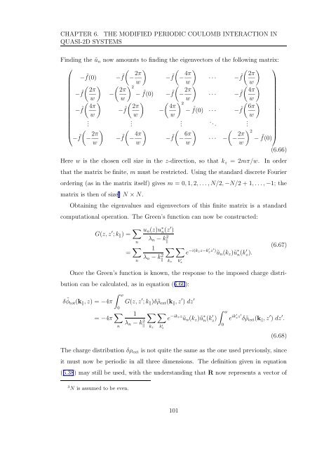
Finding the ũ n now amounts to finding the eigenvectors of the following matrix:
⎛
(
− ˜f(0) − ˜f − 2π ) (
− w
˜f − 4π )
( ) ⎞
· · · −
w
˜f 2π ( ) ( ) ˜f(
w 2 − ˜f 2π 2π
− −
w w
˜f(0) − − 2π )
( )
· · · −
w
˜f 4π ( ) ( ) ( )
w
2 ( )
− ˜f 4π
− w ˜f 2π 4π
− −
w w
˜f(0) · · · − ˜f
6π .
w .
.
.
... .
⎜ (
⎝
− ˜f − 2π ) (
−
w
˜f − 4π ) (
−
w
˜f − 6π ) (
· · · − − 2π ) 2 ⎟
−
w
w ˜f(0) ⎠
(6.66)
Here w is the chosen cell size in the z-direction, so that k z
= 2mπ/w. In order
that the matrix be finite, m must be restricted. Using the standard discrete Fourier
ordering (as in the matrix itself) gives m = 0, 1, 2, . . . , N/2, −N/2 + 1, . . . , −1; the
matrix is then of size 3 N × N.
Obtaining the eigenvalues and eigenvectors of this finite matrix is a standard
computational operation. The Green’s function can now be constructed:
G(z, z ′ ; k ‖ ) = ∑ n
= ∑ n
u n (z)u ∗ n(z ′ )
λ n − k‖
2
1 ∑ ∑
e −i(kzz−k′ zz ′)ũ
λ n − k‖
2 n (k z )ũ ∗ n(k z).
′
k z
k ′ z
(6.67)
Once the Green’s function is known, the response to the imposed charge distribution
can be calculated, as in equation (6.60):
δ ˜φ tot (k ‖ , z) = −4π
∫ w
0
= −4π ∑ n
G(z, z ′ ; k ‖ )δ ˜ρ ext (k ‖ , z ′ ) dz ′
1 ∑ ∑
∫ w
e −ikzz ũ
λ n − k‖
2 n (k z )ũ ∗ n(k z)
′ e ik′ z z′ δ ˜ρ ext (k ‖ , z ′ ) dz ′ .
0
k z
k ′ z
(6.68)
The charge distribution δρ ext is not quite the same as the one used previously, since
it must now be periodic in all three dimensions. The definition given in equation
(6.38) may still be used, with the understanding that R now represents a vector of
3 N is assumed to be even.
101