My PhD thesis - Condensed Matter Theory - Imperial College London

CHAPTER 3.
QUANTUM MONTE CARLO METHODS
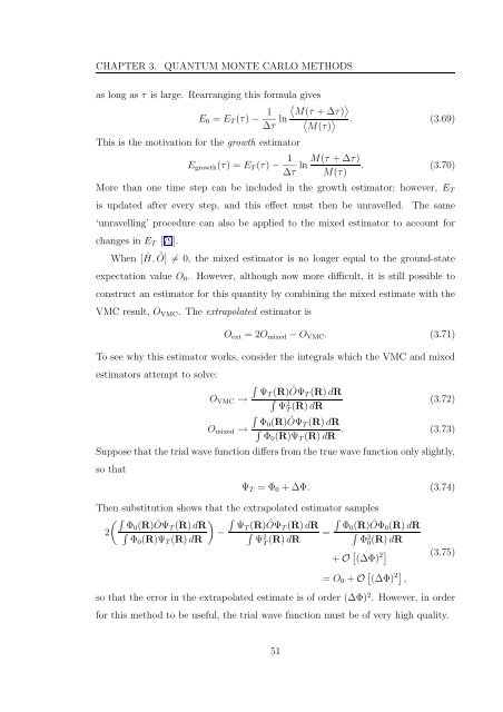
as long as τ is large. Rearranging this formula gives
This is the motivation for the growth estimator
E 0 = E T (τ) − 1
∆τ ln 〈
M(τ + ∆τ)
〉
〈
M(τ)
〉 . (3.69)
E growth (τ) = E T (τ) − 1
∆τ
M(τ + ∆τ)
ln . (3.70)
M(τ)
More than one time step can be included in the growth estimator; however, E T
is updated after every step, and this effect must then be unravelled.
The same
‘unravelling’ procedure can also be applied to the mixed estimator to account for
changes in E T [79].
When
[Ĥ, Ô] ≠ 0, the mixed estimator is no longer equal to the ground-state
expectation value O 0 . However, although now more difficult, it is still possible to
construct an estimator for this quantity by combining the mixed estimate with the
VMC result, O VMC . The extrapolated estimator is
O ext = 2O mixed − O VMC . (3.71)
To see why this estimator works, consider the integrals which the VMC and mixed
estimators attempt to solve:
O VMC →
∫
ΨT (R)ÔΨ T (R) dR
∫
Ψ
2
T
(R) dR
(3.72)
O mixed →
∫
Φ0 (R)ÔΨ T (R) dR
∫
Φ0 (R)Ψ T (R) dR . (3.73)
Suppose that the trial wave function differs from the true wave function only slightly,
so that
Ψ T = Φ 0 + ∆Φ. (3.74)
Then substitution shows that the extrapolated estimator samples
(∫
Φ0
2
(R)ÔΨ ) ∫
T (R) dR ΨT
∫ −
(R)ÔΨ ∫
T (R) dR Φ0
∫ =
(R)ÔΦ 0(R) dR
∫
Φ0 (R)Ψ T (R) dR
Ψ
2
T
(R) dR
Φ
2
0 (R) dR
+ O [ (∆Φ) 2]
(3.75)
= O 0 + O [ (∆Φ) 2] ,
so that the error in the extrapolated estimate is of order (∆Φ) 2 . However, in order
for this method to be useful, the trial wave function must be of very high quality.
51