1. Introduction 2. RETRO - AMS supported meetings

More documents

Recommendations

Info

Now the key is to determine the complex weighting function wj. A relatively simple and robust method developed by Capon (1969) was successfully applied to atmospheric radar to improve angular resolution using signals from spatially spaced receivers (Palmer et al. 1998; Yu et al. 2000), and to obtain high-resolution vertical profile of reflectivity and three-dimensional wind field using shifted frequencies (Palmer et al. 1999; Yu and Brown 2004). Using Capon’s approach, the weighting vector in RETRO can be obtained by solving the following constrained optimization. min RYj wj (0), subject to qHj wj = 1 (3) where qj is a column vector of size L specifying the weights for the true high resolution signals at the jth subvolume to produce oversampled signals in V. The optimization ensures that the effect of interference is minimized while the response of the weighting function at the jth subvolume is unity. Interference refers to signals from subvolumes other than the subvolume in which the RETRO estimation is performed. The Capon weighting vector can be derived using a Lagrange method (Capon 1969; Palmer et al. 1998; Yu et al. 2005). As a result, time series of high-resolution signals at a subvolume Yj can be generated by substituting the weighting function into (1). Reflectivity and radial velocity at subvolumes can be estimated by processing Yj(mTs), m = 0, 1, . . . M − 1,using either spectral technique or autocovariance methods (Doviak and Zrnić (1993), Chapter 6), where Ts is the pulse repetition time and M is the number of samples. Yu et al. (2005) have shown that the estimated high-resolution signal power ( ˆ Pj) is a weighted sum of the true high-resolution power σ2 l at 2L − 1 subvolumes. ˆPj = 2L−1 � l=1 Ejlσ 2 l (4) where the weight Ejl is the lth element of square of the RETRO response of the weighting function Ej, and j = 1, . . . 2L − 1. Thus, performance of high-resolution power estimate is determined by the weighting function which is adaptive to the atmospheric structure. Note that a deterministic bias in RETRO power estimate will be obtained for the case of uniform reflectivity. For example, the theoretical bias for L = 10 is approximately 7.4 dB given that the correlation of oversampled signals in range has a triangular shape (Torres and Zrnić 2003). Nevertheless, for the case of uniform reflectivity resolution is not of primary interest and the whitening-based technique may be used to improve the statistical accuracy of the estimates. Yu 2 (a) Signal power and velocity from conventional sampling y−direction (km) 5.4 5.2 5 4.8 4.6 −0.5 0 x−direction (km) 0.5 S (dB) 0 20 40 60 y−direction (km) 5.4 5.2 5 4.8 4.6 −0.5 0 x−direction (km) 0.5 V (ms −1 ) −20 0 20 (b) Signal power and velocity from RETRO y−direction (km) 5.4 5.2 5 4.8 4.6 −0.5 0 x−direction (km) 0.5 Z (dB) 0 20 40 60 y−direction (km) 5.4 5.2 5 4.8 4.6 −0.5 0 x−direction (km) 0.5 V (ms −1 ) −40 −20 0 20 40 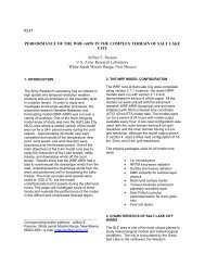Figure 1: Reflectivity and velocity fields of a tornado vortex observed by a virtual WSR-88D using (a) conventional sampling (L = 1) and (b) RETRO (L = 5). et al. (2005) have further shown that the highresolution RETRO velocity is a biased estimator except for the case of uniform velocity field. However, the bias can be significantly small such that the RETRO high-resolution velocity estimates still reflects the true velocity field. 3. Results RETRO is tested and verified using numerical simulation of a tornado vortex. Oversampled data were generated based on a simulation scheme similar to the one used in Torres and Zrnić (2003). Ideal time series were generated independently at each subvolume according to designed Doppler
spectrum as described in Zrnić (1975). In this work, tornado spectra are simulated using a combined Rankine model (Zrnić and Doviak 1975; Yu et al. 2003). Subsequently, range oversampled signals were obtained through a weighted sum of the L ideal time series. The weights are determined by the range weighting function. In this work, a rectangular pulse of 250 m is simulated to demonstrate the resolution improvement on WSR-88D. Moreover, it is assumed that receiver has a bandwidth much larger than 1/τ′, the same condition used in Torres and Zrnić (2003) and Ivić et al. (2003). A sequence of white Gaussian noise is added to each set of oversampled data according to a designed signal-to-noise ratio (SNR). In simulation, a tornado is located at 5 km north of the radar in which the diameter of the maximum wind is 100 m and the maximum tangential wind is 50 m s −1 . A doughnut-shape reflectivity with a width of 40 m is simulated and the maximum reflectivity is located at the radius of 110 m from the center of the tornado. Level I time series data collected by a virtual WSR-88D with 1 ◦ beamwidth and 250 m pulse length scanning through the tornado were simulated with and without range oversampling. The later sampling scheme is termed conventional sampling (CS) (i.e., L = 1). Both signals were generated at a constant SNR of 40 dB. The signal power and mean radial velocity from CS and RETRO with L = 5 are shown in Figure 1(a) and (b), respectively. It is clear that the reflectivity structure and velocity distribution in range are better resolved when RETRO is used. Furthermore, the range profile of signal power and radial velocity at the azimuth angle of 1 ◦ , as indicated by the white lines in Figure 1(b), is shown in Figure 2 for both CS and RETRO. The modeled signal power and radial velocity with 50 m range resolution are denoted by red lines. It is evident that RETRO can reconstruct the tornado reflectivity and velocity profile at 50 m resolution using a 250 m pulse and oversampling factor of 5. Furthermore, the performance of RETRO as a function of SNR, oversampling factor (L), and the number of samples is investigated by Yu et al. (2005). Doppler spectra reconstructed using RETRO at the subvolume of 4.8, 5.05, and 5.25 km are shown in Figure 3. The RETRO-produced and model spectra are denoted by black and red lines, respectively. It has been shown that tornado spectrum is typically broad closed to the center of tornado vortex and can be used to improve the detection (Yu et al. 2003, 2004). It is clear that not only the three spectral moments but the Doppler spectra at these subvolumes can be reconstructed us- 3 ing RETRO. Another application of RETRO is the mitigation of clutter contamination and is demonstrated in Yu et al. (2005). 4. Conclusions In this work, the application of range oversampled signals is further exploited.A technique was developed to improve range resolution using range oversampling and is termed RETRO. Improving resolution using overlapped range weighting function can be postulated as an inversion problem and the Capon method was used to solve the problem because of its simplicity and robustness. In RETRO it is assumed that high-resolution signals is a linear combination of oversampled signals. The weighting function is obtained by solving a constrained optimization. As a result, RETRO power and velocity estimates are adaptive to the oversampled data and optimal estimates can be obtained. RETRO is demonstrated using numerical simulations for a tornado case. The variation of tornado reflectivity and velocity in range was observed at resolution of subvolume using Capon RETRO, while the conventional processing techniques cannot resolve them. The result suggests that fine resolution can be achieved by transmitting a longer pulse and oversampling returns in range. However, note that the performance of RETRO is limited when the reflectivity is uniform or slowing varying in range. References Bringi, V. N. and V. Chandrasekar, 2001: Polarimetric Doppler Weather Radar Principles and Applications. Cambridge University Press, Cambridge, UK. Capon, J., 1969: High-resolution frequencywavenumber spectrum analysis. Proc. IEEE, 57, 1408–1419. Crum, T. D. and R. L. Alberty, 1993: The wsr-88d and the wsr-88d operational support facility. Bull. Amer. Meteor. Soc., 74, 1669–1687. Doviak, R. J. and D. S. Zrnić, 1993: Doppler Radar and Weather Observations. Academic, San Diego, Calif. Ivić, I. R., D. Zrnić, and S. M. Torres, 2003: Whitening in range to improve weather radar spectral moment estimates part ii: experimental evaluation. J. Atmos. Oceanic Technol., 20, 1449– 1459.
Page 1: 4R.4 IMPROVE RADAR RESOLUTION USING
Page 5: Spectrum (dB) 50 0 (a) 4.8 km 50 0

1. Introduction 2. RETRO - AMS supported meetings

You also want an ePaper? Increase the reach of your titles

Delete template?

Save as template?