MMSE Detection for Spatial Multiplexing MIMO (SM-MIMO)

KEEE494: 2nd Semester 2009 Week 12
MMSE Detection for Spatial Multiplexing MIMO (SM-MIMO)
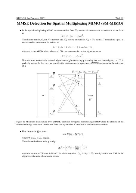
• In the spatial multiplexing MIMO, the transmit data from N T number of antennas can be written in vector form
as
x = [x 1 , x 2 , · · · , c NT ] T .
The channel matrix, G, for N T transmit and N R receive antennas is N R × N T matrix. The received signal at
the lth receive antenna can be written as
r l = g l1 x 1 + g l2 x 2 + · · · + g lNT x NT
+ n l
where n l is the AWGN with variance σ 2 . We can construct the receive signal vector as
r = [r 1 , r 2 , · · · , r NR ] T .
Now we want to detect the transmit signal vector x by observing r assuming that the channel gain, i.e., G, is
perfectly known. In this class we consider the minimum mean square error (MMSE) criterion for the detection
of x.
Figure 1: Minimum mean square error (MMSE) detection for spatial multiplexing MIMO where the element of the
channel vector g l consists of the channel from the N T number of antennas to the lth receive antenna.
• Find the matrix W to have
where W is N R × N T matrix.
The solution is shown to be given by
W H =
min E { (x − W H r) 2}
[
G H G + I ] −1
N T
G H
SNR
which is known as ”Wiener Solution”. In above equation, I NT is N T × N T identity matrix and SNR is the
signal-to-noise ratio of each data stream.
1

• General solution of minimum-mean square error detection (MMSE)
– Problem description: Let us assume we have desired signal d[n] and d[n] is corrupted somehow into u[n].
Then observing u[n] and using the linear filter W we want to detect d[n]. The problem description is
illustrated in Fig. 2.
d[n] ; desired signal
u[n] ; input signal to MMSE (or Wiener) filter which contains ”desired signal d[n]”
y[n] ; estimated d[n], i.e., ˆd[n]
As an example, u[n] = d[n] + z[n] for AWGN and u[n] = h[n]d[n] + z[n] for fading channel.
Figure 2: Problem description of Wiener filter.
Now we want to find the optimum weight vector W = [w 0 , w 1 , · · · , w K−1 ] T such that the mean-squared
error is minimized. Denote the error is defined as
where
e[n] = d[n] − y[n]
y[n] =
K−1
∑
k=0
w ∗ ku[n − k]
with w k = a k + jb k . Now let us define the cost function J as
J = E[e[n]e ∗ [n]] = E[|e[n]| 2 ].
The MMSE solution for W is given as
W ∗ = min
W [J]
– Solution:
e[n] = d[n] − y[n]
=
K−1
∑
d[n] − (a k − jb k )u[n − k]
k=0
Let us define a gradient operator ∆ k with respect to the real input a k and the imaginary part b k such as
∆ k =
Apply the operator ∆ k to the cost function J yielding
Now the MMSE solution is obtained when
∂ + j ∂ , k = 0, 1, · · · , K − 1
∂a k ∂b k
∆ k J = ∂J
∂a k
+ j ∂J
∂b k
, k = 0, 1, · · · , K − 1
∆ k J = 0 for all k = 0, 1, · · · , K − 1
2

or equivalently
[ ∂e[n]
∆ k J = E
∂a k
e ∗ [n] + ∂e∗ [n]
∂a k
e[n] + j ∂e[n]
∂b k
]
e ∗ [n] + j ∂e∗ [n]
e[n]
∂b k
Note that
Using the above, we have
or equivalently
We can rewrite it as
∂e[n]
∂a k
= −u[n − k]
∂e[n]
∂b k
= ju[n − k]
∂e ∗ [n]
∂a k
= −u ∗ [n − k]
∂e ∗ [n]
∂a k
= −ju ∗ [n − k].
∆ k J = E [ −u[n − k]e ∗ [n] − u ∗ [n − k]e[n] − u[n − k]e ∗ [n] + u ast [n − k]e[n] ]
= −2E [u[n − k]e ∗ [n]]
= 0
E[u[n − k]e ∗ [n]] = 0, k = 0, 1, · · · , K − 1
[ (
⇒
E
u[n − k]
⇒ E [u[n − k]d ∗ [n]] =
K−1
∑
l=0
d ∗ [n] −
K−1
∑
l=0
w l u ∗ [n − l]
w l E [u[n − k]u ∗ [n − l]] ,
which is called ”Wiener-Hopf equation”. Note that in the Wiener-Hope equation, the left-hand side term is
cross-correlation between u[n−k] and d[n] for a lag of −k and the right-hand side term is auto-correlation
function of the filter output for a lag of l − k. Let us express these as
φ uu (l − k) = E [u[n − k]u ∗ [n − l]]
φ ud (−k) = E [u[n − k]d ∗ [n]]
Hence, the Wiener-Hopf equation can be rewritten as
Let us define
K−1
∑
l=0
w k φ uu (l − k) = φ ud (−k), k = 0, 1, · · · , K − 1
u[n] = [u[n], u[n − 1], · · · , u[n − K + 1]] T ,
and define the correlation matrix R as
⎡
⎤
φ uu (0) φ uu (1) · · · φ uu (K − 1)
φ ∗ uu(1) φ uu (0) · · · φ uu (K − 2)
R = ⎢
.
⎥
⎣
.
⎦
φ ∗ uu(K − 1) φ ∗ uu(K − 2) · · · φ uu (0)
)]
= 0.
3

and
T = E[u[n]d ∗ [n]]
= [φ ud (0), φ ud (−1), · · · , φ ud (1 − K)] T .
Then, Wiener-Hopf equation can be rewritten as
RW = T
Finally, the Wiener solution is given as
W = R −1 T
Figure 3: Transversal linear Wiener filter.
• Now in our MIMO case which is of our interest, when we apply the Wiener solution, we have
where
ˆx 1 =
ˆx 2 =
.
x NT ˆ =
Then, from the Wiener solution, w l is given as
∑N R
wk 1∗ r k = w 1H · r
k=1
∑N R
wk 2∗ r k = w 2H · r
k=1
∑N R
w N R∗
k
r k = w N RH · r
k=1
w l = [w l 1, w l 2, · · · , w l N R
] T .
w l = R −1 T l .
Now let us find R and T . Note that R = [rr H ] which is N R × N R matrix given as
⎡
E[r 1 r1] ∗ E[r 1 r2] ∗ · · · E[r 1 r ∗ ⎤
N R
]
⎢
⎥
R = ⎣
.
⎦
E[r NR r1] ∗ E[r NR r2] ∗ · · · E[r NR rN ∗ R
]
where
r k = g k1 x 1 + g k2 x 2 + · · · + g kNT x NT + n k
= g T k x + n k
4

Hence,
E[r k r ∗ l ] = E[(g k1 x 1 + · · · + g k x NT + n k ) · (g ∗ l1x ∗ 1 + · · · + g ∗ lN T
x ∗ N T
+ n ∗ l )]
= E[g k1 g ∗ l1|x 1 | 2 + g k2 g ∗ l2|x 2 | 2 + · · · + g kNT g ∗ lN T
|x NT | 2 + g k1 g ∗ l2x 1 x ∗ 2 + · · · + g kNT g lNT −1x ∗ N T −1 + n k n ∗ l ]
Since E[x 1 x ∗ 2] = 0 and g k and g l are known, it can be rewritten as
E[r k r ∗ l ] = g k1 g ∗ l1E[|x 1 | 2 ] + g k2 g ∗ l2E[|x 2 | 2 ] + · · · + g kNT g ∗ lN T
E[|x NT | 2 ] + σ 2 δ(k − l)
Note that E[|x l | 2 ] = P is the signal power for all k. Then,
E[r k r ∗ l ] = P ( g k1 g ∗ l1 + · · · + g kNT g ∗ lN T
)
On the other hand,
⎡
= P [ gl1, ∗ gl2, ∗ · · · , glN ∗ ] T · ⎢
⎣
= P (g H l · g k ) + σ 2 δ(k − l).
g k1
g k2
.
.
g kNT
T l = E[r · x ∗ l ]
⎡ ⎤
r 1 · x ∗ l
⎢
= E ⎣
r 2 · x ∗ ⎥
l ⎦
.
.r NR · x ∗ l
⎡ ⎤
g l1 P
g l2 P
= E ⎢
⎣
⎥
. ⎦
g lNT P
= P g l ,
⎤
⎥
⎦ + σ2 δ(k − l)
where we note that r k = g k1 x 1 + g k2 x 2 + · · · + g kNT x NT . Now the MMSE solution is
w l = R −1 T l
⎛ ⎡
g H 1 · g 1 g H 2 · g 1 · · · g H ⎤ ⎞
N R · g 1
1
g H 1 · g 2 g H 2 · g 2 · · · g H N R · g 2
= ⎜ ⎢
⎝P
⎣
⎥
.
⎦ + σ2 ⎟
⎠
g H 1 · g N R
g H 2 · g 2 · · · g H N R · g NR
⎛⎡
g H 1 · g 1 g H 2 · g 1 · · · g H ⎤ ⎞−1
N R · g 1
g H 1 · g 2 g H 2 · g 2 · · · g H N R · g 2
= ⎜⎢
⎝⎣
⎥
.
⎦ + σ2
⎟
P ⎠
g H 1 · g NR
g H 2 · g 2 · · · g H N R · g NR
We can rewrite the optimal weight vector in matrix form denoted as W as
⎡
⎤
∣ ∣ ∣
W =
⎢ w 1 w 2 · · · w NR
⎥
⎣
⎦
∣ ∣ ∣
(
= G G · G H + 1 ) −1
SNR I N T
,
5
−1
g l
P g l

or
W H =
(
G H G + 1
SNR I N T
) −1
G H
6