Using IBM SPSS 19 Descriptive Statistics - CBU

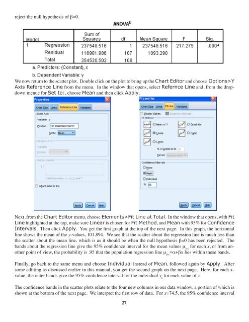
eject the null hypothesis of b=0.
We now return to the scatter plot. Double click on the plot to bring up the Chart Editor and choose Options>Y
Axis Reference Line from the menu. In the window that opens, select Refernce Line and, from the dropdown
menue for Set to:, choose Mean and then click Apply.
Next, from the Chart Editor menu, choose Elements>Fit Line at Total. In the window that opens, with Fit
Line highlighted at the top, make sure Linear is chosen for Fit Method, and Mean with 95% for Confidence
Intervals. Then click Apply. You get the first graph at the top of the next page. In this graph, the horizontal
line shows the mean of the y-values, 101.894. We see that the scatter about the regression line is much less than
the scatter about the mean line, which is as it should be when the null hypothesis b=0 has been rejected. The
bands about the regression line give the 95% confidence interval for the mean values m y|x
for each x, or from another
point of view, the probability is .95 that the population regression line m y|x
=a+bx lies within these bands.
Finally, go back to the same menu and choose Individual instead of Mean, followed again by Apply. After
some editting as discussed earlier in this manual, you get the second graph on the next page. Here, for each x-
value, the outer bands give the 95% confidence interval for the individual y I
for each value of x.
The confidence bands in the scatter plots relate to the four new columns in our data window, a portion of which is
shown at the bottom of the next page. We interpret the first row of data. For x=74.5, the 95% confidence interval
27