Using IBM SPSS 19 Descriptive Statistics - CBU
Using IBM SPSS 19 Descriptive Statistics - CBU
Using IBM SPSS 19 Descriptive Statistics - CBU

You also want an ePaper? Increase the reach of your titles
YUMPU automatically turns print PDFs into web optimized ePapers that Google loves.
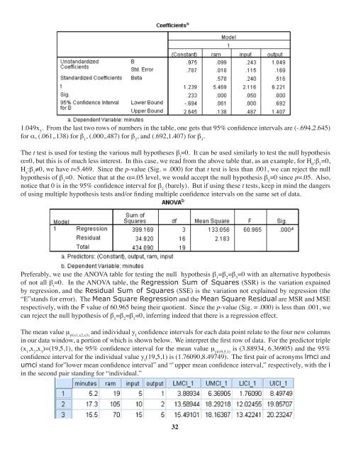
1.049x 3<br />
. From the last two rows of numbers in the table, one gets that 95% confidence intervals are (-.694,2.645)<br />
for a, (.061,.138) for b 1<br />
, (.000,.487) for b 2<br />
, and (.692,1.407) for b 3<br />
.<br />
The t test is used for testing the various null hypotheses b i<br />
=0. It can be used similarly to test the null hypothesis<br />
a=0, but this is of much less interest. In this case, we read from the above table that, as an example, for H 0<br />
:b 1<br />
=0,<br />
H a<br />
:b 1<br />
≠0, we have t=5.469. Since the p-value (Sig. = .000) for that t test is less than .001, we can reject the null<br />
hypothesis of b 1<br />
=0. Notice that at the a=.05 level, we would accept the null hypothesis b 2<br />
=0 since p=.05. Also,<br />
notice that 0 is in the 95% confidence interval for b 2<br />
(barely). But if using these t tests, keep in mind the dangers<br />
of using multiple hypothesis tests and/or finding multiple confidence intervals on the same set of data.<br />
Preferably, we use the ANOVA table for testing the null hypothesis b 1<br />
=b 2<br />
=b 3<br />
=0 with an alternative hypothesis<br />
of not all b i<br />
=0. In the ANOVA table, the Regression Sum of Squares (SSR) is the variation expained<br />
by regression, and the Residual Sum of Squares (SSE) is the variation not explained by regression (the<br />
“E”stands for error). The Mean Square Regression and the Mean Square Residual are MSR and MSE<br />
respectively, with the F value of 60.965 being their quotient. Since the p-value (Sig. = .000) is less than .001, we<br />
can reject the null hypothesis of b 1<br />
=b 2<br />
=b 3<br />
=0, inferring indeed that there is a regression effect.<br />
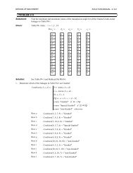
The mean value m y|(x1,x2,x3)<br />
and individual y I<br />
confidence intervals for each data point relate to the four new columns<br />
in our data window, a portion of which is shown below. We interpret the first row of data. For the predictor triple<br />
(x 1<br />
,x 2<br />
,x 3<br />
)=(<strong>19</strong>,5,1), the 95% confidence interval for the mean value m y|(<strong>19</strong>,5,1)<br />
is (3.88934, 6.36905) and the 95%<br />
confidence interval for the individual value y I<br />
(<strong>19</strong>,5,1) is (1.76090,8.49749). The first pair of acronyms lmci and<br />
umci stand for”lower mean confidence interval” and “`upper mean confidence interval,” respectively, with the i<br />
in the second pair standing for “individual.”<br />
32