Geant4 Simulations for the Radon Electric Dipole Moment Search at
Geant4 Simulations for the Radon Electric Dipole Moment Search at
Geant4 Simulations for the Radon Electric Dipole Moment Search at

Create successful ePaper yourself
Turn your PDF publications into a flip-book with our unique Google optimized e-Paper software.
distribution, this average intensity can increase or decrease over <strong>the</strong> depolariz<strong>at</strong>ion<br />
time. The 416 keV M1 transition shown in Figure 4.5(b) clearly illustr<strong>at</strong>es this effect.<br />
Even though <strong>the</strong> number of nuclei inside <strong>the</strong> cell, and hence <strong>the</strong> total activity is<br />
decreasing, <strong>the</strong> observed average count r<strong>at</strong>e increases over <strong>the</strong> depolariz<strong>at</strong>ion time<br />
scale (which is short compared to <strong>the</strong> 223 Rn half-life of 24.3 minutes). This change<br />
in <strong>the</strong> average count r<strong>at</strong>e occurs because <strong>the</strong> “donut shaped” distribution depolarizes<br />
into an isotropic distribution th<strong>at</strong> has a larger average γ-ray intensity in <strong>the</strong> plane of<br />
<strong>the</strong> eight GRIFFIN detectors. This effect is fur<strong>the</strong>r studied in Figures 4.6 and 4.7.<br />
The remaining terms describe <strong>the</strong> precession, where A 5 is <strong>the</strong> frequency, A 6 is <strong>the</strong><br />
phase and A 7 , A 8 , A 9 , ··· are <strong>the</strong> intensities of odd-sine oscill<strong>at</strong>ions. A maximum of<br />
14 odd-sine terms were included into <strong>the</strong> fitting program (up to A 20 ), however, often<br />
only <strong>the</strong> first few odd-sine terms were non-zero. In this case all o<strong>the</strong>r sine terms fixed<br />
to zero and removed from <strong>the</strong> fit.<br />
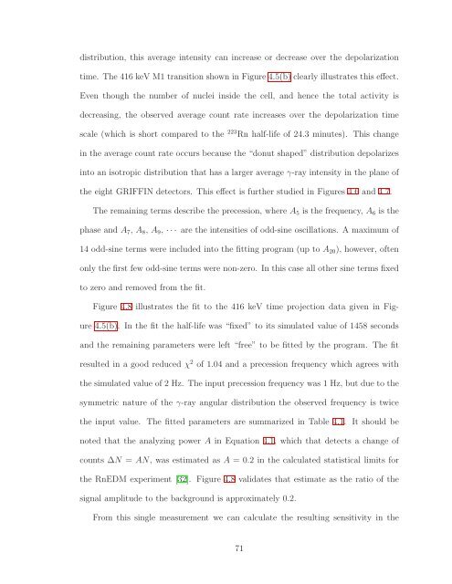
Figure 4.8 illustr<strong>at</strong>es <strong>the</strong> fit to <strong>the</strong> 416 keV time projection d<strong>at</strong>a given in Figure<br />
4.5(b). In <strong>the</strong> fit <strong>the</strong> half-life was “fixed” to its simul<strong>at</strong>ed value of 1458 seconds<br />
and <strong>the</strong> remaining parameters were left “free” to be fitted by <strong>the</strong> program. The fit<br />
resulted in a good reduced χ 2 of 1.04 and a precession frequency which agrees with<br />
<strong>the</strong> simul<strong>at</strong>ed value of 2 Hz. The input precession frequency was 1 Hz, but due to <strong>the</strong><br />
symmetric n<strong>at</strong>ure of <strong>the</strong> γ-ray angular distribution <strong>the</strong> observed frequency is twice<br />
<strong>the</strong> input value. The fitted parameters are summarized in Table 4.1. It should be<br />
noted th<strong>at</strong> <strong>the</strong> analyzing power A in Equ<strong>at</strong>ion 4.1, which th<strong>at</strong> detects a change of<br />
counts ∆N = AN, was estim<strong>at</strong>ed as A = 0.2 in <strong>the</strong> calcul<strong>at</strong>ed st<strong>at</strong>istical limits <strong>for</strong><br />
<strong>the</strong> RnEDM experiment [32]. Figure 4.8 valid<strong>at</strong>es th<strong>at</strong> estim<strong>at</strong>e as <strong>the</strong> r<strong>at</strong>io of <strong>the</strong><br />
signal amplitude to <strong>the</strong> background is approxim<strong>at</strong>ely 0.2.<br />
From this single measurement we can calcul<strong>at</strong>e <strong>the</strong> resulting sensitivity in <strong>the</strong><br />
71