Introduction to LabVIEW Control Design Toolkit by Finn Haugen ...

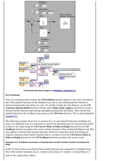
Front panel and block diagram of feedback_connection.vi.
End of Example
Note: For continuous-time models, the CD Feedback function ignores a time delay included in
any of the transfer functions in the feedback loop, that is, the resulting transfer function is
derived assuming the time delays are zero. To actually include the time delay(s), use the CD
Construct Special Model function with the option Delay (Pade Approx.) selected to create a
rational transfer function representing (and approximating) the time delay. Then include this
transfer function in the feedback loop using e.g. the CD Series function. This is demonstrated in
Example 9.1.
The following example shows how to connect discrete-time transfer functions including time
delays in a feedback loop. It is necessary to convert the time delay part of a discrete-time model
to poles at the origin using the CD Convert Delay to Poles at Origin function for the CD
Feedback function to produce the correct transfer function of the combined feedback loop. This
also applies to discrete-time transfer functions which have been derived by discretizing an
original continuous-time transfer function, that is, you have to use the CD Convert Delay to
Poles at Origin function for the CD Feedback function to produce the correct result.
Example 4.2.2: Feedback connection of discrete-time transfer function models including time
delay
In the VI shown below two discrete-time transfer functions are connected in a feedback loop.
One of the transfer functions, H 2
(z), contains a time delay of 2 samples, corresponding to 2
poles at the origin of the z-plane.