Introduction to LabVIEW Control Design Toolkit by Finn Haugen ...

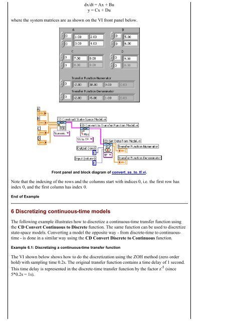
dx/dt = Ax + Bu
y = Cx + Du
where the system matrices are as shown on the VI front panel below.
Front panel and block diagram of convert_ss_to_tf.vi.
Note that the indexing of the rows and the columns start with indices 0, i.e. the first row has
index 0, and the first column has index 0.
End of Example
6 Discretizing continuous-time models
The following example illustrates how to discretize a continuous-time transfer function using
the CD Convert Continuous to Discrete function. The same function can be used to discretize
state-space models. Converting a model the opposite way - from discrete-time to continuoustime
- is done in a similar way using the CD Convert Discrete to Continuous function.
Example 6.1: Discretizing a continuous-time transfer function
The VI shown below shows how to do the discretization using the ZOH method (zero order
hold) with sampling time 0.2s. The original transfer function contains a time delay of 1 second.
This time delay is represented in the discrete-time transfer function by the factor z -5 (since
5*0.2s = 1s).