Introduction to LabVIEW Control Design Toolkit by Finn Haugen ...

Norm
Covariance Response
Total Delay
Distribute Delay
Parametric Time Response
The State Space Model Analysis palette, with the following functions:
Controllability Matrix
Observability Matrix
Grammians
Canonical State-Space Realization
Balance State-Space Model (Diagonal)
Balance State-Space Model (Grammians)
Controllability Staircase
Observability Staircase
State Similarity Transform
The State Feedback Design palette, with the following functions:
Ackermann
Pole Placement
Linear Quadratic Regulator
Kalman Gain
State Estimator
State-Space Controller
Augment Output with States
3 Creating models
3.1 Creating and displaying continuous-time (s-)transfer functions
The Model Construction palette contains several functions for creating models. The resulting
model is represented as a cluster. This cluster can be used as input argument to other functions,
e.g. for simulation, frequency response analysis, etc.
On the Model Construction palette there are also functions for displaying the transfer function
nicely on the front panel.
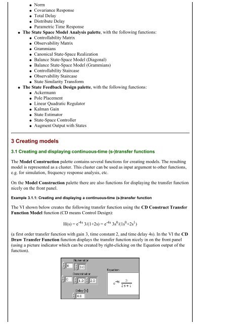
Example 3.1.1: Creating and displaying a continuous-time (s-)transfer function
The VI shown below creates the following transfer function using the CD Construct Transfer
Function Model function (CD means Control Design):
H(s) = e -4s 3/(1+2s) = e -4s 3s 0 /(1s 0 +2s 1 )
(a first order transfer function with gain 3, time constant 2, and time delay 4s). In the VI the CD
Draw Transfer Function function displays the transfer function nicely in on the front panel
(using a picture indicator which can be created by right-clicking on the Equation output of the
function).