Vehicle Crashworthiness and Occupant Protection - Chapter 3

Vehicle Crashworthiness and Occupant Protection
challenge to the analyst. Numerical techniques, at this time, appear to be the
practical option.
The FE method of structural dynamics solves numerically a set of nonlinear partial
differential equations of motion in the space-time domain, coupled with material
stress-strain relations along with definition of appropriate initial and boundary
conditions. The solution first discretizes the equations in space by formulating
the problem in a weak variational form and assuming an admissible displacement
field. This yields a set of second order differential equations in time. Next, the
system of equations is solved by discretization in the time domain. The
discretization is accomplished by the classical Newmark-Beta method [29]. The
technique is labeled implicit if the selected integration parameters render the equations
coupled, and in this case the solution is unconditionally stable. If the integration
parameters are selected to decouple the equations, then the solution is
labeled explicit, and it is conditionally stable. Earlier developments in nonlinear FE
technology used primarily implicit solutions [30]. FE simulation for structural crashworthiness
by explicit solvers appears to be first introduced by Belytschko [11].
Later, Hughes et al [31] discussed the development of mixed explicit-implicit solutions.
The explicit FE technique solves a set of hyperbolic wave equations in the zone
of influence of the wave front, and accordingly does not require coupling of large
numbers of equations. On the other hand, the unconditionally stable implicit
solvers provide a solution for all coupled equations of motion, which require
assembly of a global stiffness matrix. The time step for implicit solvers is about
two to three orders of magnitude of the explicit time step. For crash simulations
involving extensive use of contact, multiple material models and a combination of
non-traditional elements, it turned out that explicit solvers are more robust and
computationally more efficient than implicit solvers.
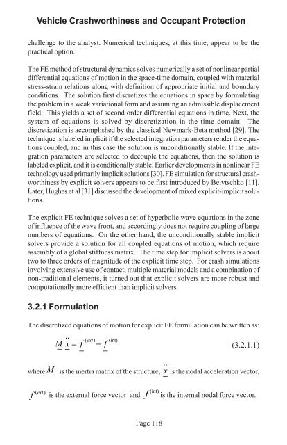
3.2.1 Formulation
The discretized equations of motion for explicit FE formulation can be written as:
..
( ext)
(int)
M x = f − f
− −
(3.2.1.1)
− −
..
where M −
is the inertia matrix of the structure, x is the nodal acceleration vector,
−
(ext)
f is the external force vector and
f
(int)
is the internal nodal force vector.
Page 118