Introduction to Categorical Data Analysis

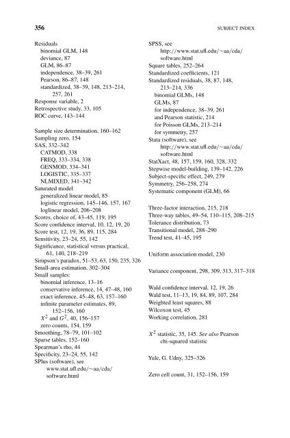
356 SUBJECT INDEX
Residuals
binomial GLM, 148
deviance, 87
GLM, 86–87
independence, 38–39, 261
Pearson, 86–87, 148
standardized, 38–39, 148, 213–214,
257, 261
Response variable, 2
Retrospective study, 33, 105
ROC curve, 143–144
Sample size determination, 160–162
Sampling zero, 154
SAS, 332–342
CATMOD, 338
FREQ, 333–334, 338
GENMOD, 334–341
LOGISTIC, 335–337
NLMIXED, 341–342
Saturated model
generalized linear model, 85
logistic regression, 145–146, 157, 167
loglinear model, 206–208
Scores, choice of, 43–45, 119, 195
Score confidence interval, 10, 12, 19, 20
Score test, 12, 19, 36, 89, 115, 284
Sensitivity, 23–24, 55, 142
Significance, statistical versus practical,
61, 140, 218–219
Simpson’s paradox, 51–53, 63, 150, 235, 326
Small-area estimation, 302–304
Small samples:
binomial inference, 13–16
conservative inference, 14, 47–48, 160
exact inference, 45–48, 63, 157–160
infinite parameter estimates, 89,
152–156, 160
X 2 and G 2 , 40, 156–157
zero counts, 154, 159
Smoothing, 78–79, 101–102
Sparse tables, 152–160
Spearman’s rho, 44
Specificity, 23–24, 55, 142
SPlus (software), see
www.stat.ufl.edu/∼aa/cda/
software.html
SPSS, see
http://www.stat.ufl.edu/∼aa/cda/
software.html
Square tables, 252–264
Standardized coefficients, 121
Standardized residuals, 38, 87, 148,
213–214, 336
binomial GLMs, 148
GLMs, 87
for independence, 38–39, 261
and Pearson statistic, 214
for Poisson GLMs, 213–214
for symmetry, 257
Stata (software), see
http://www.stat.ufl.edu/∼aa/cda/
software.html
StatXact, 48, 157, 159, 160, 328, 332
Stepwise model-building, 139–142, 226
Subject-specific effect, 249, 279
Symmetry, 256–258, 274
Systematic component (GLM), 66
Three-factor interaction, 215, 218
Three-way tables, 49–54, 110–115, 208–215
Tolerance distribution, 73
Transitional model, 288–290
Trend test, 41–45, 195
Uniform association model, 230
Variance component, 298, 309, 313, 317–318
Wald confidence interval, 12, 19, 26
Wald test, 11–13, 19, 84, 89, 107, 284
Weighted least squares, 88
Wilcoxon test, 45
Working correlation, 281
X 2 statistic, 35, 145. See also Pearson
chi-squared statistic
Yule, G. Udny, 325–326
Zero cell count, 31, 152–156, 159