EQUATIONS OF ELASTIC HYPERSURFACES

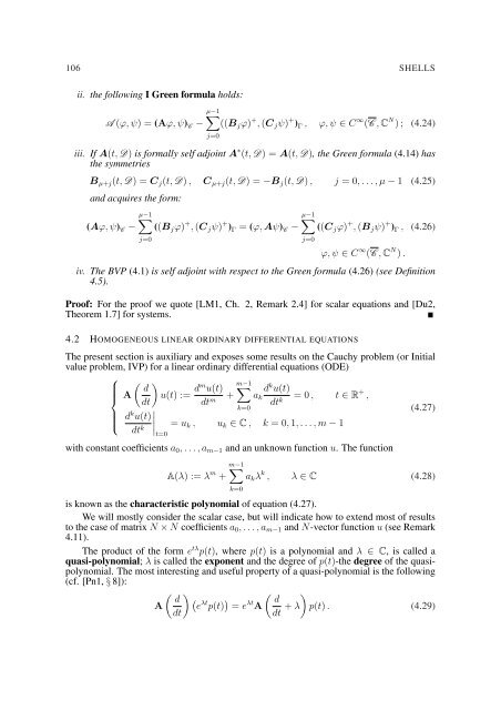
106 SHELLS
ii. the following I Green formula holds:
µ−1
∑
A (ϕ, ψ) = (Aϕ, ψ) C − ((B j ϕ) + , (C j ψ) + ) Γ , ϕ, ψ ∈ C ∞ (C , C N ) ; (4.24)
j=0
iii. If A(t, D) is formally self adjoint A ∗ (t, D) = A(t, D), the Green formula (4.14) has
the symmetries
B µ+j (t, D) = C j (t, D) , C µ+j (t, D) = −B j (t, D) , j = 0, . . . , µ − 1 (4.25)
and acquires the form:
µ−1
µ−1
∑
∑
(Aϕ, ψ) C − ((B j ϕ) + , (C j ψ) + ) Γ = (ϕ, Aψ) C − ((C j ϕ) + , (B j ψ) + ) Γ , (4.26)
j=0
j=0
ϕ, ψ ∈ C ∞ (C , C N ) .
iv. The BVP (4.1) is self adjoint with respect to the Green formula (4.26) (see Definition
4.5).
Proof: For the proof we quote [LM1, Ch. 2, Remark 2.4] for scalar equations and [Du2,
Theorem 1.7] for systems.
4.2 HOMOGENEOUS LINEAR ORDINARY DIFFERENTIAL EQUATIONS
The present section is auxiliary and exposes some results on the Cauchy problem (or Initial
value problem, IVP) for a linear ordinary differential equations (ODE)
⎧ ( d
⎪⎨ A u(t) :=
dt)
dm m−1
u(t)
dt + ∑ d k u(t)
a m
k = 0 , t ∈ R + ,
dt k
⎪⎩
k=0
d k u(t)
dt k ∣
∣∣∣t=0
= u k , u k ∈ C , k = 0, 1, . . . , m − 1
with constant coefficients a 0 , . . . , a m−1 and an unknown function u. The function
A(λ) := λ m +
m−1
∑
k=0
(4.27)
a k λ k , λ ∈ C (4.28)
is known as the characteristic polynomial of equation (4.27).
We will mostly consider the scalar case, but will indicate how to extend most of results
to the case of matrix N × N coefficients a 0 , . . . , a m−1 and N-vector function u (see Remark
4.11).
The product of the form e tλ p(t), where p(t) is a polynomial and λ ∈ C, is called a
quasi-polynomial; λ is called the exponent and the degree of p(t)-the degree of the quasipolynomial.
The most interesting and useful property of a quasi-polynomial is the following
(cf. [Pn1, § 8]):
( ) d (e
A
λt p(t) ) ( ) d
= e λt A
dt
dt + λ p(t) . (4.29)