EQUATIONS OF ELASTIC HYPERSURFACES

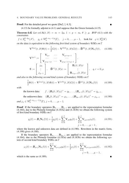
4. BOUNDARY VALUE PROBLEMS: GENERAL RESULTS 143
Proof: For the detailed proof we quote [Du2, § 6.3].
(4.13) be formally adjoint to (4.1) and suppose that the Green formula (4.15)
Theorem 4.42 Let ord A(t, D) = m = 2µ, 1 < p < ∞, θ ≥ µ. BVP (4.1) with the
constraints
f ∈ X θ−2µ
p (S ) , g j ∈ W θ−m j−1/p
p (Γ) , j = 0, . . . , µ − 1, look for ϕ ∈ X θ p(C )
on the data is equivalent to the following first kind system of boundary ΨDEs on Γ
V (0,µ) (t, D)Φ(t) = 1 2 G(t) − V(0,0) (t, D)G(t) − ˜B (0) (t, D)N C f(t) , (4.188)
⎡
V (q,r) := ⎣
Φ :=
⎡
⎢
⎣
⎤
V q,r · · · V q,r+µ−1
· · · · · · · · · ⎦ ,
V q+µ−1,r · · · V q+µ−1,r+µ−1
⎤
ϕ 0
⎥
.
ϕ µ−1
⎦ , ˜B (r) (t, D)ψ :=
⎡
⎢
⎣
B r (t, D)ψ
.
B r+µ−1 (t, D)ψ
⎤
⎥
⎦ , q, r = 0, µ
and also to the following second kind system of boundary ΨDEs on Γ
1
2 Φ(t) − V(µ,µ) (t, D)Φ(t) = V (µ,0) (t, D)G(t) + ˜B (µ) (t, D)N C f(t) (4.189)
with
the known data: f , (B 0 (t, D)ϕ) + = g 0 , . . . , (B µ−1 (t, D)ϕ) + = g µ−1 ,
the unknown data: (B µ (t, D)ϕ) + = ϕ 0 , . . . , (B 2µ−1 (t, D)ϕ) + = ϕ µ−1 (4.190)
and ϕ j ∈ W θ−m µ+j−1/p
p (Γ), j = 0, . . . , µ − 1.
Proof: If the boundary operators B 0 , . . . , B µ−1 are applied to the representation formulae
(4.164), due to the Plemelji formulae (4.183a) and (4.183b) we obtain the following system
of first kind boundary ΨDEs on Γ
g j (t) = B j N C f(t) + 1 µ−1
µ−1
2 g ∑ ∑
j(t) + V jk g k (t) + V j,µ+k ϕ k (t) , (4.191)
k=0
k=0
j = 0, . . . , µ − 1 ,
where the known and unknown data are defined in (4.190). Rewritten in the matrix form,
(4.190) gives (4.188).
If the boundary operators B µ , . . . , B 2µ−1 are applied to the representation formulae
(4.164), due to the Plemelji formulae (4.183a) and (4.183b) we obtain the following system
of second kind boundary ΨDEs on Γ
µ−1
∑
ϕ j (t) = B µ+j N C f(t) + V µ+j,k g k (t) + 1 µ−1
2 ϕ ∑
j(t) + V µ+j,µ+k ϕ k (t) , (4.192)
which is the same as (4.189).
k=0
k=0
j = 0, . . . , µ − 1 ,