EQUATIONS OF ELASTIC HYPERSURFACES

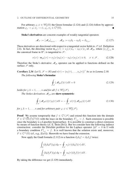
2. OUTLINE OF DIFFERENTIAL GEOMETRY 35
For arbitrary ϕ, ψ ∈ W 1 2(Ω) the Green formulae (2.124) and (2.124) follow by approximation
ϕ j → ϕ, ψ j → ψ, ϕ j , ψ j ∈ C 2 (Ω).
Stoke’s derivatives are concrete examples of weakly tangential operators
M S := [M jk ] n×n
, M jk := ν j ∂ k − ν k ∂ j = ∂ mj,k . (2.127)
These derivatives are directional with respect to a tangential vector fields to S (cf. Definition
2.4). In fact, the directing vector m jk (X ) = ν j (X )e k − ν k (X )e j of M jk , where {e j } n j=1 is
the canonical frame in R n , is tangential to S :
ν(X ) · m jk (X ) = ν j (X )ν k (X ) − ν k (X )ν j (X ) ≡ 0, X ∈ S . (2.128)
Therefore the Stoke’s derivative M jk operator can be applied to functions defined on the
surface S only.
Corollary 2.34 Let Ω, S = ∂Ω and ν(τ) = (ν 1 (τ), . . . , ν n (τ)) ⊤ be as in Lemma 2.30.
The following Stoke’s formulae
∮
(M jk f)(τ) dS = 0 (2.129)
S
holds for j, k = 1, . . . , n and for all f ∈ W 1 1(S ).
The Stokes derivatives M j,k are skew-symmetric:
∮
∮
(M jk ψ)(τ)ϕ(τ) dS = − ψ(τ)(M jk ϕ)(τ) dS (2.130)
S
S
for j, k = 1, . . . , n and for arbitrary pair ϕ, ψ ∈ W 2 2(S ).
Proof: We assume temporarily that f ∈ C 1 (S ) and extend this function into the domain
F ∈ C 1 (Ω) ⋂ C 2 (Ω) with the trace on the boundary F ∣ S
= f. Such extension is possible
since the boundary is a Lipschitz hypersurface. It is possible to construct a direct extension
by means of function theory (cf. E. Stein [St1]). But we consider here the following indirect
construction: consider the Dirichlet problem for the Laplace operator ∆F = 0 in Ω with
a boundary condition F ∣ S
= f. It is well known that the solution exists and, moreover,
F ∈ C ∞ (Ω) (cf., e.g., [Le1]). Herewith we have found the extension.
Now apply the Gauß formula (2.112) to a function ∂ j ∂ k f = ∂ k ∂ j f twice:
∫
∮
(∂ j ∂ k F )(y) dy = ν j (τ)(∂ k f)(τ) dS ,
∫
Ω
Ω
∮
(∂ k ∂ j F )(y) dy =
By taking the difference we get (2.129) immediately.
S
S
ν k (τ)(∂ j f)(τ) dS .