EQUATIONS OF ELASTIC HYPERSURFACES

More documents

Recommendations

Info

4 SHELLS The form is correctly defined because the differential operator ∂ V is tangential and can be applied to a function f defined on the surface S only. Then, for a given f, there exists a vector field ∇ S f ∈ TS such that ω f (V ) := 〈∇ S f, V 〉 for all V ∈ V (X) , (1.3) which is, classical differential geometry, the definition of surface Gradient of a function f ∈ C 1 (S ) and maps ∇ S : C ∞ (S ) → TS . (1.4) The surface divergence Div S : V (S ) → C ∞ (S ) (1.5) of a smooth tangential vector field is, by the definition, the dual operator with the opposite sign 〈Div S V, f〉 := −〈V, ∇ S f〉 , ∀ V ∈ TS , ∀ f ∈ C 1 (S ) . (1.6) Expressing these operators in intrinsic parameters of the surface S (tangential vector fields, Metric tensor etc.) one obtains (cf. [Ca1, Ci4, Ku1, Ta2]): Div S U := [ det G S ] −1/2 n∑ j=1 { [det ] } 1/2U ∑ j ∂ j GS = n ∇ S f = ∑ j,k (gjk ∂ j f) ∂ k . j=1 U j ;j = Tr ∇ S U , (1.7) where U j ;k denotes the componentwise covariant derivative, while ∇ S U is the tensor field defined by the covariant derivative (∇ S U)V := ∂U S V (see § 2.7 and [Ta2, Ch. 2, § 3]). Their composition is the Laplace-Beltrami operator ∆ S f := Div S ∇ S f = [ ] −1/2 ∑n−1 det G S which is self-adjoint due to (1.5): j,k=1 ∂ j {g jk[ ] } 1/2∂k det G S f , f ∈ C 2 (S ) , (1.8) ∆ ∗ S = ( ∇ S Div S ) ∗ = ( DivS ) ∗ ( ∇S ) ∗ = ∇S Div S = ∆ S . (1.9) The intrinsic parameters enable generalization to arbitrary manifolds, not necessarily immersed in the Euclidean space R n . On the other hand it is sometimes more convenient to record these operators in cartesian coordinates. For example, it is easy to ascertain that the surface gradient is nothing but the collection of the weakly tangential Günter’s (covariant) derivatives ∇ S = D S := (D 1 , . . . , D n ) ⊤ , D j := ∂ j − ν j (X )∂ ν = ∂ dj , (1.10) where ∂ ν := ∑ n j=1 ν j∂ j denotes the normal derivative (cf. [Gu1], [KGBB1], [Du1]). Here, for each 1 ≤ j ≤ n, the first-order differential operator D j = ∂ dj is the directional derivative along the tangential vector d j := π S e j . The operator (the matrix) π S : R n → TS , π S (t) = I − ν(t)ν ⊤ (t) = [ δ jk − ν j (t)ν k (t) ] n×n , t ∈ S (1.11)
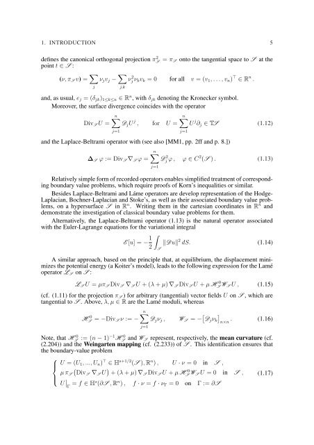
1. INTRODUCTION 5 defines the canonical orthogonal projection π 2 S = π S onto the tangential space to S at the point t ∈ S : (ν, π S v) = ∑ j ν j v j − ∑ j,k ν 2 j ν k v k = 0 for all v = (v 1 , . . . , v n ) ⊤ ∈ R n . and, as usual, e j = (δ jk ) 1≤k≤n ∈ R n , with δ jk denoting the Kronecker symbol. Moreover, the surface divergence coincides with the operator Div S U = n∑ D j U j , for U = j=1 n∑ U j ∂ j ∈ TS (1.12) and the Laplace-Beltrami operator with (see also [MM1, pp. 2ff and p. 8.]) ∆ S ϕ := Div S ∇ S ϕ = j=1 n∑ Dj 2 ϕ , ϕ ∈ C 2 (S ) . (1.13) j=1 Relatively simple form of recorded operators enables simplified treatment of corresponding boundary value problems, which require proofs of Korn’s inequalities or similar. Besides Laplace-Beltrami and Láme operators are develop representation of the Hodge- Laplacian, Bochner-Laplacian and Stoke’s, as well as their associated boundary value problems, on a hypersurface S in R n . Writing them in the cartesian coordinates in R n and demonstrate the investigation of classical boundary value problems for them. Alternatively, the Laplace-Beltrami operator (1.13) is the natural operator associated with the Euler-Lagrange equations for the variational integral E [u] = − 1 ∫ ‖Du‖ 2 dS. (1.14) 2 A similar approach, based on the principle that, at equilibrium, the displacement minimizes the potential energy (a Koiter’s model), leads to the following expression for the Lamé operator L S on S : S L S U = µπ S Div S ∇ S U + (λ + µ) ∇ S Div S U + µ H 0 S W S U , (1.15) (cf. (1.11) for the projection π S ) for arbitrary (tangential) vector fields U on S , which are tangential to S . Above, λ, µ ∈ R are the Lamé moduli, whereas H 0 S = −Div S ν := − n∑ D j ν j , W S = − [ D j ν k ]n×n . (1.16) j=1 Note, that HS 0 := (n − 1)−1 HS 0 and W S represent, respectively, the mean curvature (cf. (2.204)) and the Weingarten mapping (cf. (2.233)) of S . This identification ensures that the boundary-value problem ⎧ ⎪⎨ ⎪⎩ U = (U 1 , ..., U n ) ⊤ ∈ H s+1/2 (S ), R n ) , U · ν = 0 in S , µ π S ( DivS ∇ S U ) + (λ + µ) ∇ S Div S U + µ H 0 S W S U = 0 in S , U ∣ ∣ Γ = f ∈ H s (∂S , R n ) , f · ν = f · ν Γ = 0 on Γ := ∂S (1.17)
Page 1 and 2: Grant GNSF/ST06/3-001 of the Georgi
Page 3: 1. INTRODUCTION 3 1 INTRODUCTION Pa
Page 7 and 8: 2. OUTLINE OF DIFFERENTIAL GEOMETRY
Page 55 and 56:
2. OUTLINE OF DIFFERENTIAL GEOMETRY
Page 57 and 58:
Page 59 and 60:
Page 61 and 62:
Page 63 and 64:
Page 65 and 66:
3. CALCULUS OF DIFFERENTIAL OPERATO
Page 67 and 68:
Page 69 and 70:
Page 71 and 72:
Page 73 and 74:
Page 75 and 76:
Page 77 and 78:
Page 79 and 80:
Page 81 and 82:
Page 83 and 84:
Page 85 and 86:
Page 87 and 88:
Page 89 and 90:
Page 91 and 92:
Page 93 and 94:
Page 95 and 96:
Page 97 and 98:
Page 99 and 100:
Page 101 and 102:
4. BOUNDARY VALUE PROBLEMS: GENERAL
Page 103 and 104:
Page 105 and 106:
Page 107 and 108:
Page 109 and 110:
Page 111 and 112:
Page 113 and 114:
Page 115 and 116:
Page 117 and 118:
Page 119 and 120:
Page 121 and 122:
Page 123 and 124:
Page 125 and 126:
Page 127 and 128:
Page 129 and 130:
Page 131 and 132:
Page 133 and 134:
Page 135 and 136:
Page 137 and 138:
Page 139 and 140:
Page 141 and 142:
Page 143 and 144:
Page 145 and 146:
Page 147 and 148:
5. BOUNDARY VALUE PROBLEMS: EXAMPLE
Page 149 and 150:
Page 151 and 152:
Page 153 and 154:
Page 155 and 156:
Page 157 and 158:
Page 159 and 160:
Page 161 and 162:
Page 163 and 164:
Page 165 and 166:
Page 167 and 168:
Page 169 and 170:
Page 171 and 172:
Page 173 and 174:
Page 175 and 176:
Page 177 and 178:
Page 179 and 180:
Page 181 and 182:
BIBLIOGRAPHY 181 [CD1] O.Chkadua, R
Page 183 and 184:
BIBLIOGRAPHY 183 [Hr1] L. Hörmande
Page 185:
BIBLIOGRAPHY 185 [Si1] I. Simonenko
show all

EQUATIONS OF ELASTIC HYPERSURFACES

You also want an ePaper? Increase the reach of your titles

Delete template?

Save as template?