EQUATIONS OF ELASTIC HYPERSURFACES
EQUATIONS OF ELASTIC HYPERSURFACES
EQUATIONS OF ELASTIC HYPERSURFACES

Create successful ePaper yourself
Turn your PDF publications into a flip-book with our unique Google optimized e-Paper software.
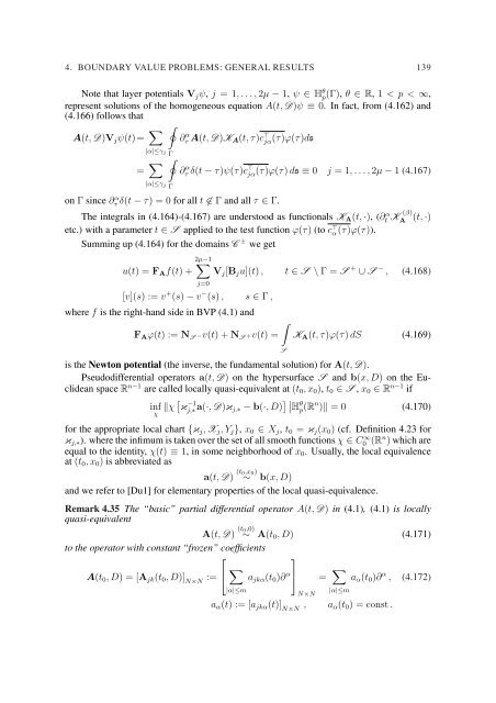
4. BOUNDARY VALUE PROBLEMS: GENERAL RESULTS 139<br />
Note that layer potentials V j ψ, j = 1, . . . , 2µ − 1, ψ ∈ H θ p(Γ), θ ∈ R, 1 < p < ∞,<br />
represent solutions of the homogeneous equation A(t, D)ψ ≡ 0. In fact, from (4.162) and<br />
(4.166) follows that<br />
A(t, D)V j ψ(t)= ∑ ∮<br />
∂τ α A(t, D)K A (t, τ)c ⊤ jα (τ)ϕ(τ)ds<br />
|α|≤γ j<br />
Γ<br />
= ∑<br />
|α|≤γ j<br />
∮<br />
Γ<br />
on Γ since ∂ α τ δ(t − τ) = 0 for all t ∉ Γ and all τ ∈ Γ.<br />
∂τ α δ(t − τ)ψ(τ)c ⊤ jα (τ)ϕ(τ) ds ≡ 0 j = 1, . . . , 2µ − 1 (4.167)<br />
The integrals in (4.164)-(4.167) are understood as functionals K A (t, ·), (∂t α K (β)<br />
A<br />
(t, ·)<br />
etc.) with a parameter t ∈ S applied to the test function ϕ(τ) (to c ⊤ α (τ)ϕ(τ)).<br />
Summing up (4.164) for the domains C −+ we get<br />
u(t) = F A f(t) +<br />
2µ−1<br />
∑<br />
j=0<br />
[v](s) := v + (s) − v − (s) , s ∈ Γ ,<br />
where f is the right-hand side in BVP (4.1) and<br />
∫<br />
F A ϕ(t) := N S −v(t) + N S +v(t) =<br />
V j [B j u](t) , t ∈ S \ Γ = S + ∪ S − , (4.168)<br />
S<br />
K A (t, τ)ϕ(τ) dS (4.169)<br />
is the Newton potential (the inverse, the fundamental solution) for A(t, D).<br />
Pseudodifferential operators a(t, D) on the hypersurface S and b(x, D) on the Euclidean<br />
space R n−1 are called locally quasi-equivalent at (t 0 , x 0 ), t 0 ∈ S , x 0 ∈ R n−1 if<br />
inf<br />
χ<br />
‖χ [ κ −1<br />
j,∗ a(·, D)κ j,∗ − b(·, D) ] ∣ ∣H θ p(R n )‖ = 0 (4.170)<br />
for the appropriate local chart {κ j , X j , Y j }, x 0 ∈ X j , t 0 = κ j (x 0 ) (cf. Definition 4.23 for<br />
κ j,∗ ). where the infimum is taken over the set of all smooth functions χ ∈ C0 ∞ (R n ) which are<br />
equal to the identity, χ(t) ≡ 1, in some neighborhood of x 0 . Usually, the local equivalence<br />
at (t 0 , x 0 ) is abbreviated as<br />
a(t, D) (t 0,x 0 )<br />
∼ b(x, D)<br />
and we refer to [Du1] for elementary properties of the local quasi-equivalence.<br />
Remark 4.35 The “basic” partial differential operator A(t, D) in (4.1), (4.1) is locally<br />
quasi-equivalent<br />
A(t, D) (t 0,0)<br />
∼ A(t 0 , D) (4.171)<br />
to the operator with constant “frozen” coefficients<br />
⎡<br />
⎤<br />
A(t 0 , D) = [A jk (t 0 , D)] N×N<br />
:= ⎣ ∑<br />
a jkα (t 0 )∂ α ⎦ = ∑<br />
a α (t 0 )∂ α , (4.172)<br />
|α|≤m<br />
N×N<br />
|α|≤m<br />
a α (t) := [a jkα (t)] N×N<br />
, a α (t 0 ) = const .