Transient integral boundary layer method to calculate the ...

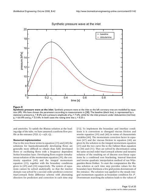
BioMedical Engineering OnLine 2006, 5:42http://www.biomedical-engineering-online.com/content/5/1/42 Synthetic Figure 8 pressure wave at the inletSynthetic pressure wave at the inlet. Synthetic pressure wave at the inlet to the left coronary tree are modelled by equation(49). We have chosen the parameters according to measurements in [38]. The baseline (black line), is represented by astationary pressure p s = 8 kPa and a pressure amplitude of p 0 = 7 kPa, while for the inlet pressure under dobutamine (red line)p s = 6.6 kPa and p 0 = 5.5 kPa. In both cases the raising time was t r = 0.25 s.and arterioles. To satisfy the Blasius solution at the leadingedge of the tube, we have assumed a uniform flow profileat the entrance (V(0, t) = u(0, t)).Numerical implementationDue to the non-linear terms in equation (23) and (40) thesolutions for haemodynamically developing flows aregenerally more difficult to obtain than fully developedflows or oscillating flows with a frequency dependentStokes boundary layer. Developing flows require simultaneoussolution of the momentum equation (39), the continuityequation (40) and the integral momentumequation (23), together with the boundary conditionsgiven in (49) and (24) respectively. The system of equationscannot be solved analytically, so that the interiordomain was solved by a second order predictor-correctorMacCormack finite difference scheme with alternatingdirection for prediction and correction in each time step[72]. To implement the boundary and interface conditionsit is convenient to disregard viscous friction andrewrite equation (39) and (40) in terms of characteristicvariables [46]. The momentum correction factor in equation(47) and the viscous friction in equation (48) aregiven by the solution to the integral momentum equation(23) and the two curve fits to the Falkner-Skan equationin (30) and (31). They are solved by discretisation usingthe same second order MacCormack scheme and iterativesolution of the resulting set of discrete non-linear equationsby a combined root bracketing, interval bisectionand inverse quadratic interpolation method of van Wijngaarden-Brent-Dekker.To start the computation the Blasiussolution at each time step provides values for theboundary layer thickness a few grid points downstream ofthe entrance. The solution was applied to the steady integralmomentum equation as boundary condition for δ*.Downstream marching the solution leads to the values ofPage 12 of 25(page number not for citation purposes)