Transient integral boundary layer method to calculate the ...

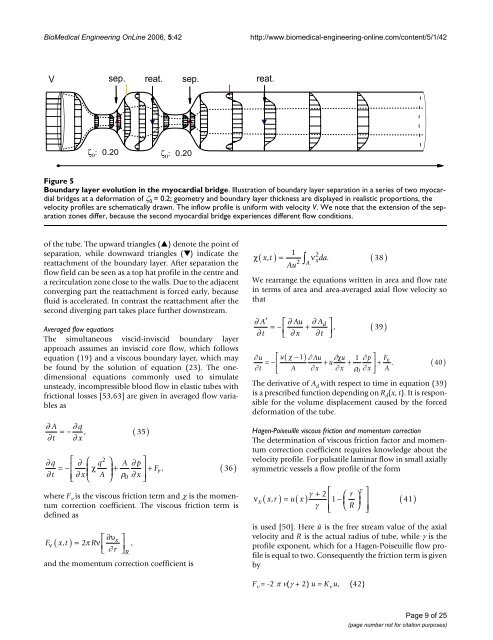
BioMedical Engineering OnLine 2006, 5:42http://www.biomedical-engineering-online.com/content/5/1/42 Boundary Figure 5 layer evolution in the myocardial bridgeBoundary layer evolution in the myocardial bridge. Illustration of boundary layer separation in a series of two myocardialbridges at a deformation of ζ 0 = 0.2; geometry and boundary layer thickness are displayed in realistic proportions, thevelocity profiles are schematically drawn. The inflow profile is uniform with velocity V. We note that the extension of the separationzones differ, because the second myocardial bridge experiences different flow conditions.of the tube. The upward triangles (▲) denote the point ofseparation, while downward triangles (▼) indicate thereattachment of the boundary layer. After separation theflow field can be seen as a top hat profile in the centre anda recirculation zone close to the walls. Due to the adjacentconverging part the reattachment is forced early, becausefluid is accelerated. In contrast the reattachment after thesecond diverging part takes place further downstream.Averaged flow equationsThe simultaneous viscid-inviscid boundary layerapproach assumes an inviscid core flow, which followsequation (19) and a viscous boundary layer, which maybe found by the solution of equation (23). The onedimensionalequations commonly used to simulateunsteady, incompressible blood flow in elastic tubes withfrictional losses [53,63] are given in averaged flow variablesas∂ A∂ t∂ q, 35∂ x=− ( )∂ q ⎡ ∂ ⎛=−⎢∂ t ∂x⎜⎣⎢⎝2χ qA⎞ A ∂ p⎟ +⎤⎥⎠ρ0∂ x⎦F v⎥ + ,( 36 )where F ν is the viscous friction term and χ is the momentumcorrection coefficient. The viscous friction term isdefined as⎡ ∂υx⎤Fν( x, t) = 2π Rν⎢ ,⎣ ∂ r⎥⎦and the momentum correction coefficient isRχ1 2xt , ∫ νx Auda .2 A( ) = ( 38 )We rearrange the equations written in area and flow ratein terms of area and area-averaged axial flow velocity sothat∂ A′ ⎡ ∂ Au ∂ A=− +∂ t⎢⎣ ∂ x ∂ t( )d⎤, 39⎦⎥ ( )∂ u ⎡ u χ −1 ∂ Au ∂χu1 ∂ p ⎤ F=−⎢+ u +ν .∂ t ⎣ A ∂ x ∂xρ0∂ x ⎦ A⎥ + ( 40 )The derivative of A d with respect to time in equation (39)is a prescribed function depending on R d (x, t). It is responsiblefor the volume displacement caused by the forceddeformation of the tube.Hagen-Poiseuille viscous friction and momentum correctionThe determination of viscous friction factor and momentumcorrection coefficient requires knowledge about thevelocity profile. For pulsatile laminar flow in small axiallysymmetric vessels a flow profile of the form( ) = ( )ν x xr , u x+ ⎡ r− ⎛ γγ 2⎝ ⎜⎞ ⎤⎢ 1 ⎟ ⎥ 41γ R⎣⎢⎠⎦⎥( )is used [50]. Here û is the free stream value of the axialvelocity and R is the actual radius of tube, while γ is theprofile exponent, which for a Hagen-Poiseuille flow profileis equal to two. Consequently the friction term is givenbyF ν = -2 π ν(γ + 2) u = K ν u, (42)Page 9 of 25(page number not for citation purposes)