etude de la qualite des eaux d'un hydrosysteme fluvial ... - LTHE

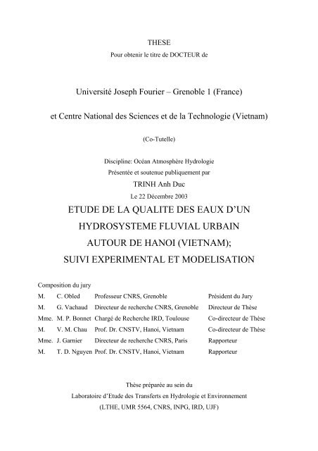
THESISFor obtaining the doctorate degree ofUniversity Joseph Fourier – Grenoble 1 (France)and National Center for Natural Science and Technology (Vietnam)(Co-supervision)Discipline: Ocean Atmosphere HydrologyWritten and defended byTRINH Anh DucDecember 22 nd 2003STUDY OF WATER QUALITY OF A URBAN RIVERHYDRO SYSTEMIN THE PERIPHERY OF HANOI (VIETNAM);EXPERIMENTS AND MODELLINGComposition of juryM. C. Obled Professor CNRS, Grenoble PresidentM. G. Vachaud Researching director CNRS, Grenoble PromoterMme. M. P. Bonnet Researcher CNRS, ToulouseCo-promoterM. V. M. Chau Prof. Dr. CNSTV, Hanoi, Vietnam Co-promoterMme. J. Garnier Researching director CNRS, Paris ReporterM. T. D. Nguyen Prof. Dr. CNSTV, Hanoi, Vietnam ReporterThe thesis is prepared at the Laboratory in research of Transfers in Hydrology andEnvironment (LTHE, UMR 5564, CNRS, INPG, IRD, UJF)

RESUMÉ EXTENSIFCette thèse s’attache à l’étude d’un problème environnemental très caractéristique de l’Asiedu Sud Est : la pollution d’hydrosystème liée au développement rapide, et généralementincontrôlé, de grandes métropoles le long de fleuves et de rivières. Faute de systèmesatisfaisant de collecte, et de traitement des eaux, et du développement en périphérie de cesvilles de méthodes d’agriculture intensive, ces hydrosystèmes reçoivent des chargespolluantes concentrées (égouts, rejets industriels ou rejets hospitaliers) ou diffuses(ruissellement d’azote ou de pesticides) qui conduisent à une détérioration marquée de laqualité des eaux. Des exemples typiques au Vietnam sont la rivière Saigon dans sa traverséede HoChiMinh Ville, la rivière des Parfums à Hué et l’hydrosystème du Fleuve Rouge autourde Hanoi.C’est pour mieux comprendre les processus de pollution de ces hydrosystèmes, et leurs effetssur la santé, notamment par le passage des polluants dans la chaîne alimentaire, qu’unprogramme de recherche multidisciplinaire a été lancé en 1999 entre équipes françaises etvietnamiennes dans le cadre d’un projet conjoint entre le Centre national de la RechercheScientifique (CNRS) et son homologue Vietnamien le Centre National pour la Science et laTechnologie du Vietnam (NCSTV). Ce programme a reçu un important soutien desorganismes, du Ministère des Affaires Etrangères, Paris, de l’Ambassade de France, Hanoi, duGroupe Sénatorial France Vietnam, Paris et du Ministère de la Science, de la Technologie etde l’Environnement (MOSTE), Hanoi. Une zone atelier, concentrant toutes les équipes sur unmême site, a pu être installée sur un site très représentatif en banlieue de Hanoi afin d’obtenirle maximum d’information permettant d’atteindre cet objectif. Ce travail, réalisé avec lesoutien d’un Bourse BDI-PED du CNRS, s’inscrit dans ce contexte et s’est attaché aux pointssuivants :1. analyse critique de 3 ans de mesure afin de caractériser l’état du système et d’élaborer unebase de données2. adaptation et validation d’un modèle écologique existant dans le but d’identifier lesprocessus les plus importants responsables de la pollution du milieu

3. utilisation de ce modèle pour émettre des suggestions d’aménagements pouvant conduire àune amélioration du systèmeJe tiens à noter le rôle essentiel qu’a joué dans cette étude Nicolas PRIEUR, volontairescientifique international, qui a assuré la coordination locale de ce projet, et notammentl’organisation des campagnes de mesure et le suivi des analyses.

1.2. Construction d’une base de donnéesCe réseau fluvial de Nhue-To Lich a déjà été étudié précédemment en particulier par leDOSTE (Département de la science, technologie et environnement de Hanoi) et le JICA(Agence Japonaise de Coopération) de 1990 jusqu’en 1999. Plusieurs enquêtes de terrain,avec mesures de la qualité des eaux sur les points fixes et représentatifs ont été effectuées,mais les résultats obtenus ne sont ni systématiques et ni synchronisées (les mesureshydrauliques, chimiques et biologiques n’ont pas été effectuées en même temps). Le nombred’observations, et d’échantillonnage sont épars, et manquent de cohérence et de régularité. Defait, les informations obtenues par ces mesures sont partielles et localisées, et ne permettentpas de caractériser les processus essentiels relatifs à la dégradation des eauxPour éviter ces défauts, ce nouveau programme Franco-vietnamien s’est d’abord concentrésur la construction d’un plan d’échantillonnage permettant d’avoir un schéma cohérent etreprésentatif de mesures sur une zone bien définie. Sur cette zone, les pointsd’échantillonnage ont été fixés et répartis d’une façon régulière, avec des échantillonnagesmensuels concernant le régime hydraulique, météorologique ainsi que les variables physiques,chimiques et biologiques permettant de caractériser qualité des eaux.En parallèle avec ce plan d’échantillonnage trois stations fixes permettant d’avoir des mesuresen continues ont été construites autour du point de confluence. Ces 3 stations sont lessuivantes(1) Cau Den, près de la ville de Ha Dong, sur le fleuve Nhue, à 5 km de l’aval de laconfluence.(2) Thanh Liet, sur le fleuve To Lich, à 300 m l’amont de la confluence(3) Khê Tang, sur le fleuve Nhue, à 5 km à l’aval de la confluenceChacune de ces stations a été équipée d’un prélever automatique et d’une sondemultiparamètres (pH, Température, Turbidité, NH 4 , Oxygène Dissous, Redox, Conductivité)connectée à une centrale d’acquisition. L’objectif de cette installation est d’obtenir lesinformations permettant d’identifier l’impact des apports de pollution massive de la rivière ToLich sur la qualité de l’eau de la Nhue. Il faut noter qu’à l’aval de la confluence, de

L’ensemble de ces indices permet d’apprécier l’évolution de qualité de l’eau de la rivièreNhue par les éléments internes ou externes.1.3. Fonctionnement hydraulique et pollution nutritiveLe fonctionnement hydraulique du système est entièrement contrôlé par une série de barrages.D’abord le barrage de Thuy Phuong, situé sur le Fleuve Nhue juste au niveau de la prise surle Fleuve Rouge qui limite les apports vers la Nhue, notamment en temps de forte crue ; puis,au niveau de la ville de Ha Dong, à 15 kms au sud, le barrage de Cau Den qui est lerégulateur essentiel de la portion d’étude du Fleuve Nhue sur laquelle va se concentrer notreétude, et qui a pour rôle d’assurer un drainage correct de l’agglomération de Hanoi. Puis sur laTo Lich, juste avant son embouchure avec la Nhue, le barrage de Thanh Liet, qui permetd’éviter les remontées d’eau vers Hanoi, et qui a été détruit en cours d’étude pour donner lieuà la construction d’un autre barrage plus moderne. Enfin, à l’aval sur la Nhue, à 40 kms auSud du fleuve Rouge, le barrage de Dong Quan. On notera que du fait de l’endiguementancien de la Nhue il n’y a pas de liaison hydraulique entre la rivière et la plaine environnante :l’irrigation des rizières et le drainage sont assurés par des systèmes de pompage ou de siphon.Une partie notable de notre travail a porté sur l’élaboration de courbes de tarage , obtenues àpartir d’un grand nombre de mesures de débits effectuées sur des profils en travers en bateauéquipé d’un système de mesure par ADCP (Accoustic Doppler current profile) au droit desbarrages de Thuy Phuong, Cau Den et Dong Quan, sur lesquels on dispose d’échellelimnomètriques. L’analyse des mesures de débit a clairement mis en évidence l’importancedes apports latéraux, de type diffus (de l’ordre de 20.000m 3 /jour pour un débit nominal del’ordre de 180.000m 3 /jour) avec généralement de forte charge polluante.L’analyse en terme de qualité nous a conduit a considérer deux sections différentes : d’unepart depuis le Fleuve Rouge jusqu’à l’arrivée de la rivière To Lich, où l’on observe unedégradation croissante vers l’aval de la qualité de l’eau , sans toutefois atteindre de seuilcritique, puis la section en aval de la To Lich qui atteint un régime très critique. En période defaible débit, le teneur en NH 4 y atteint 5mg N/l, la valeur de DO est quasi nulle, la BODaugmente jusqu’à 50mg O 2 /l. Dans cette section, du fait du mélange et des processusbiologiques, la qualité s’améliore vers l’aval, mais la zone d’observation n’est pas assez

étendue pour déterminer la limite de pollution. Il est toutefois clair qu’en période de faibledébit la pollution s’étend sur au moins 25 kmsNous nous sommes également attaché à caractériser les fluctuations temporelles de la qualitéde l’eau soit au niveau saisonnier soit au niveau journalier. Les résultats obtenus sur le plansaisonnier montrent qu’il n’existe pas , à cette échelle, de tendance identifiable, sinon uneinfluence du régime hydraulique (notamment la mousson) et de la charge polluante amenéepar la To Lich . L’analyse de la variabilité journalière de la qualité des eaux est fondée sur lesmesures réalisées à l’aide des stations automatiques et concerne essentiellement l’oxygène, lepH et NH4. D’une manière générale, le cycle journalier de la qualité des eaux n’a pas uneamplitude très marquée et est fortement influencé par les conditions hydrologiques. Il estcependant significatif à partir d’expérimentations menées sur le fleuve Rouge et il sembledevoir être attribué à des processus biologiques (le cycle est synchrone au cycle jour/nuit)..Les expérimentations menées directement sur la Nhue sont par contre plus difficiles àinterpréter, car les variations ne sont pas synchrones au cycle du soleil. Deux hypothèses sontavancées pour expliquer ce décalage dans le temps :- Première hypothèse, la variation diurne enregistrée résulte d’une activité biologique prenantplace en amont du point de mesure, et le décalage dans le temps correspond au temps detransit de l’eau entre ce point amont et le point de mesure.- Deuxième hypothèse, la variation diurne enregistrée reflète une variation journalière desapports latéraux, principalement d’origine domestique.Cependant, compte tenu des données disponibles, il ne nous est pas possible d’aller plus loindans l’interprétation

2. Modélisation du système fluvial Nhue-To LichCompte tenu de la configuration du site étudié, et des données disponibles une approche 1Dlongitudinale a été retenue. La modélisation a été menée à l’aide du logiciel AQUASIM dontla flexibilité, en particulier dans la définition des variables et des processus à simuler nous aparu particulièrement adapté à notre problème.Afin de pouvoir contraindre relativement bien le modèle, la zone étudiée a été restreinte à untronçon de la rivière Nhue d’une quarantaine de kilomètres depuis sa source (dérivationdepuis le fleuve rouge jusqu’à environ 15 km en aval de la confluence avec la rivière To-Lich) ; la rivière To Lich constitue dans ce système un apport direct. Une fois établies lesconditions limites de débit en amont du tronçon étudié et de hauteur d’eau en aval, le logicielAQUASIM résout les équations de St Venant en régime permanent ou transitoire.Le schéma conceptuel pour les aspects bio géochimique repose sur celui du modèle RWQM1(Reichert et al., 2000). Ce schéma prend en compte l’activité des micro-organismesautotrophes (bactéries nitrifiantes, algues) et des bactéries hétérotrophes et leur impacts surl’évolution de l’oxygène, du carbone organique, de l’azote (ammonium et nitrate) et duphosphore. En outre le modèle permet la simulation des matières en suspension (encaractérisant les processus de déposition et de remise en suspension), du pH par la prise encompte explicite des principaux couples acide-base. Enfin, le modèle inclut l’influence defacteurs environnementaux tel que le vent, la température et l’ensoleillement.Ce modèle, après vérification, a été appliqué tout d’abord en régime permanent, afin decaractériser, par la modélisation, le comportement moyen annuel de la rivière Nhue. Lesconditions limites (flux entrant à l’amont, flux latéraux et apport direct par la To-Lych) ontété définies à partir des données mensuelles collectées en 2002 et moyennées sur 1 an. Lesrésultats des simulations ont été comparés aux données mensuelles moyenne récoltées le longde la rivière Nhue en 2002. Cette comparaison a permis la calibrage de la plupart desparamètres cinétiques du modèle, selon la méthode proposée par (Brun et al, 2001) bien

adaptée au modèle proposé. Les valeurs obtenues pour les paramètres les plus sensibles dumodèle sont en bon accord avec les données de littérature, et les résultats du modèle sontcohérents avec les observations, malgré les nombreuses simplifications introduites dans lamodélisation. Afin de vérifier la robustesse du modèle, celui-ci a été validé à partir desdonnées mensuelles récoltées en 2003. Là encore, les résultats restent cohérents et restituentcorrectement les grandes tendances observées pour les différentes variables dans le systèmeétudié.Le modèle a ensuite été appliqué en régime transitoire. Cependant, compte tenu de la naturetrès parcellaire des données récoltées, le régime transitoire n’a pu être étudié que pour uneportion réduite de la rivière Nhue, d’une étendue d’une vingtaine de kilomètres comprise enle barrage Cau Den (emplacement de la station de mesure automatique amont) et le barrageDong Quan (la station de mesure automatique aval étant située quelque peu en amont de cebarrage). De même, seuls quelques jours consécutifs ont pu être étudiés, les stations demesure en continu ne pouvant pas fonctionner en continu sans surveillance humaine. Lacalibration du modèle établie en régime permanent a été vérifiée, la plupart des paramètresrestant invariant. La simulation en régime transitoire a été validée à l’aide de donnéescollectées en 2003. Les simulations en régime transitoires permettent de mettre en évidence laforte augmentation de l’activité des bactéries hétérotrophes au sein de la rivière Nhue après laconfluence avec la rivière To Lich ainsi que l’influence fondamentale des paramètreshydrologiques et hydrométéorologiques sur la qualité de l’eau dans le système étudié.

3. Caractéristiques principales de l’écosystème etpropositions d’aménagement3.1. Caractéristiques principales de l’écosystèmeUne fois le modèle calibré et validé, il est possible de quantifier les flux de matière entre lesdifférents compartiments du système (compartiments biotiques et abiotiques). Ce type decalcul permet facilement de mettre en évidence les principaux processus qui gouvernentl’évolution des variables-clefs dans le système étudié. Une étude détaillée de ces flux pour lesdeux principales variables du modèle a été réalisée. Les résultats soulignent, d’une part, lecaractère hétérotrophe de la rivière Nhue, les termes de production d’oxygène dissous dans lemilieu étant inférieurs à ceux de consommation. De plus, il est aisément mis en évidence, uneintensification importante des activités autotrophes et hétérotrophes entre les tronçons amontet aval de la confluence avec la rivière To-Lych. Dans le cas de l’oxygène, l’activité estenviron trois fois supérieure en aval de la confluence.Ce type de calcul permet également une comparaison entre différents écosystèmes. Lesrésultats obtenus pour la rivière Nhue ont ainsi été comparés à la Seine, pour tenter dedégager les différences de réactions entre systèmes tropicaux et tempérés, face à un apportmassif de polluant. Les résultats montrent tout d’abord que la Nhue est beaucoup plus polluéeque la Seine, même en aval de la station d’épuration d’Achères qui traite les effluentsparisiens. D’une façon générale, les processus de restauration de la qualité des eaux(dégradation aérobic, nitrification) semblent plus rapides dans la rivière Nhue que dans larivière Seine. Par contre, compte tenu de la turbidité importante des eaux, la productiond’oxygène par photosynthèse est plus faible dans la Nhue, la principale source d’oxygèneprovenant de l’atmosphère.

3.2. Propositions d’aménagement pour la rivière NhueLà également, la modélisation, une fois calée et validée permet de quantifier l’impact sur lesystème étudié de différents scénarios d’aménagement. Différents scénarios ont été simulésdans le cadre de ce travail. Une partie de ces scénarios concerne l’influence sur la qualité deseaux, des débits transitant dans la rivière Nhue. Une autre est destinée à évaluer l’impactd’une ou plusieurs stations d’épuration le long de la rivière Nhue, en période de basses eauxou hautes eaux. Il est évident que le traitement des eaux de la To Lich doit être une priorité,une station classique assurant le traitement de 335 000 m 3 /jour est suffisante, à condition quele transit dans la station soit suffisant. Cependant, compte tenu du rôle non négligeable despollutions diffuses sur la rivière Nhue, il sera nécessaire, dans un second temps, de traiter cetype de pollution, par la mise en place, par exemple de petites unités le long de la rivière.En conclusion, ce travail a tiré profit de l’ensemble des données acquises au cours duprogramme. La base de donnée ainsi constituée a permis de mettre en place un modèle bienadapté pour la description du comportement de la rivière Nhue. Cependant, tout au long de cetravail, il a fallu faire face à un certains nombre de difficultés, la principale étant le manque defiabilité des données analysées. Nous avons donc été conduit à introduire un certain nombred’hypothèses simplificatrices, qui si elles n’influent pas ou peu sur les résultats du modèlereproduisant le comportement moyen du système, s’avèrent extrêmement limitatives pour desétudes plus fines. En particulier, le comportement de la rivière par temps de pluie n’a pas puêtre étudié de façon réellement satisfaisante. Cependant, ce travail a justement permis demettre en évidence les lacunes de la base de données et le modèle pourrait être utiliser pourétudier précisément la fréquence des données nécessaire pour traiter ce type de problème.Enfin il est clair que ce type de modèle peut être utilisé comme outil d’aide à la décision enpermettant d’élaborer différents scénarios d’aménagement et en jugeant de leur efficacité faceau problème posé.

ForewordsThis thesis pursues an environmental study that is very characteristic in the South East Asia:the pollution of the hydro-systems due to rapid and uncontrollable development ofmetropolitan cities along the rivers. Due to the lack of sanitation network and wastewatertreatment wastewater, the hydro-systems are loaded with point source pollutants (sewers,industrial and hospital wastes) or non point source pollutants (fertilizes or pesticides) whichlead to a significant deterioration of the water quality. Typical examples in Vietnam are theSaigon river at its crossing of Ho Chi Minh city, the Perfume river at Hue city and the Redriver system around Hanoi city.In order to better understand the pollution processes of these hydro-systems, and their effectson health, in particular by the transport of the pollutants in the food chain, a multidisciplinaryresearch program of French and Vietnamese groups within the framework of a cooperationproject between the National Scientific Research Center (CNRS) of France and itsVietnamese counterpart the National Center for Science and Technology of Vietnam(NCSTV) was launched in 1999. The program has received important supports from differentorganisms; the Ministry of Foreign Affairs, Paris, The Embassy of France in Hanoi, senatorialgroup Vietnam France, Paris, and the Ministry of Science, Technology and Environment(MOSTE), Hanoi. A river basin representing the environmental pollution in the suburbs ofHanoi was selected for this study. All participating groups in the program have cooperated toobtain maximum information in order to achieve theses objectives. This work, completed withthe financial support of BDI-PED of CNRS, has been done within this context in order toaddress the following points1. Analysis of the 3 year measurement period to characterize the environmental state of thesystem and construct a database2. Adaptation and validation of one ecological model in order to identify the most importantprocesses governing the pollution of the water quality3. Utilization of the model to propose some suggestions for management purposes of asustainable environmental system

AcknowledgmentsFirst of all, I would like to express my many thanks to my promoters: Prof. Dr. GeorgesVachaud, French coordinator of this “French- Vietnamese Program for Water Quality andWater Treatment, FVWQT”, Dr. Marie Paule Bonnet, and Prof. Dr. CHAU Van Minh, forgiving me the opportunity to work with them and for supervising me whole-heartedlythroughout my research, and to the Vietnamese coordinator of FVWQT, Prof. NGUYEN TheDong, for integrating me in this program.I would like to express my gratitude Mr. Nicolas PRIEUR, scientific volunteer, who wasresponsible for the local coordination, field work organization and analytical management ofthe FVWQT program in Vietnam. Besides, I want to send my appreciation to all researchgroups of the FVWQT as well as other individuals and organizations who shared with mevaluable information in improvement this research.My thanks are also going to staff members of the laboratory “Etude des transferts enHydrologie et Environment” (LTHE- UMR 5564, CNRS- INPG- UJF- IRD), who haveassisted me warmly since I started to carry out this thesis.I am also highly appreciated the help of M.Sc. VU Duc Loi and other staff of the AnalyticalChemistry Laboratory (Institute of Chemistry, NCST, Hanoi, [Vietnam]), whom I mostlycollaborated with on the field works and data collection during my missions in Vietnam.In accomplishing this research I am indebted to CNRS (Centre National de la RechercheScientifique), particularly Mrs. Annie Caillat, for a fruitfully financial support.Many thanks are sent to all Vietnamese and French friends for their mental and physical helpsduring the period of this work achievement.Finally, I am deeply grateful to my wife and my family who patiently encourage me to pursuethe study.Grenoble, December 2003

Principal contentsIntroduction 1Presentation of the study 5Modelling of the Nhue-To Lich river system 63Discussion 167Conclusion and perspectives 203Annexes 207References 253

IntroductionA great challenge for natural and social scientists in the past, present, and future is tounderstand how ecological systems evolve through the bio-geo-physico-chemical interactionswithin the systems and with human beings. Our efforts to solve these problems are generallyidentified as ecological management.The ecological river management is based on monitoring, assessment and modelling of thewater evolution in river system. The choice of appropriate, high quality monitoring techniquesis a crucial factor in the assessment of river systems since they face challenges not evidence inthe precision and broaden of the available monitoring equipment. The high quality monitoringtechniques are outcome of predefined and consistent objectives, well-maintenance equipment,concrete methods, long term measurements and skillful data collection and handing.However, in many cases, the monitoring techniques are improved due to upgraded knowledgeof spatial-temporal evolution of collected data but the keen objectives should be unfailing.The development of ecological models is critical to provide useful inputs to river waterquality management strategies that will result in more efficient river water utilizationarrangements, by preventing development pressure on the river system, reducing resource useand emissions of pollutants, and minimizing impacts on ecosystems. A successful ecologicalmodel assists the analysis of actual situation of the water body (its actual condition), thequantitative assessment of deficits, determination of potential measures, the analysis andselection of conservation and/or restoration scenarios, the implementation of measures.In practice, the construction of ecological river models is largely driven by legislation andregulations (Shanahan, 1998). For U.S. framework, the most widely known and usedcomputer program for river water quality modelling is the QUAL2E model developed by theU.S. EPA (Brown and Barnwell, 1987). QUAL2E is intended specifically for the steadystreamflow, steady-effluent-discharge conditions specified in the water quality regulations forwastewater load allocation and its formulation derives directly from the U.S. regulatory1

framework for which it was developed and for which it is generally well suited. QUAL2Ethus has clear limitations such as storm water flow events and other situations with unsteadyhydraulics cannot be modelled.In Europe, water quality modelling approach is different. For municipal discharges, the EUrequirements emphasize effluent criteria set for “normal” and “sensitive” areas (which aredefined based on eutrophication potential). Decision makers typical employ dilution ratios(based on simple mass balances for the discharges to a river stretch) to assess expected waterquality. Therefore, modelling the quantity of flow in the river is generally more importantthan modelling the quality. UK environmental agencies use simple stochastic models (e.g.SIMCAT [NRA, 1990]) to summarize the two-week survey data typically collected by theagencies and to help the agencies decide on future restoration activities or permits/consentsfor dischargers on the catchment scale. Monte Carlo simulation is incorporated in theprocedure to compensate for the inherently large uncertainty in the sparse data set. Also, inthe UK, the Urban Pollution Management (UPM) procedure (FWR, 1994) has been developedand relies upon a suite of quality models of different levels of complexity, ranging fromsimple steady-state calculations implemented via a spreadsheet, to fully dynamic waterquantity and quality models. The Danish Engineering Union was early to publish a detailedprocedure for computation and assessment of water pollution, focusing on intermittent oxygendepletion due to combined sewer overflow (Spildevandskomiteen, 1985). In Germany, theATV is currently developing a comprehensive water quality model (ATV, 1996). In a numberof countries, there is a similar increasing emphasis on modelling and water quality models areincreasingly being used on a case-by-case basis for specific environmental impactassessments or scenario analysis.In France, the RIVERSTRAHER model has been developed primarily under the frameworkof the interdisciplinary program on the PIREN-Seine and lately widely used to other riversystems in Europe such as the Moselle, Loire, Scheldt, and Danube. WithRIVERSTRAHLER, the modellers can simulate the ecological functioning of drainagenetworks at the scale of their basin (Billen et al., 1994; Garnier et al., 1995). The modellingapproach requires, for each of the sub-basins, the knowledge of a number of constraints. Thegeomorphology, describing the hydrological network according to the ordination intoStrahler’s orders allows the calculation of various characteristics of each order (length, width,2

- The adaptation and validation of an ecological model in order to shed light on themain processes leading to water quality degradation; This model is discussed in partII.- The use of this model to study the particular functioning of tropical systems and to testsome management scenario. This work is presented in part III of this manuscript.I wish here to mention that whole this work would not have been possible without a tightcooperation between the different research teams and to underline the very efficient work ofNicolas Prieur, scientific voluntary, who ensured the local coordination of the program inVietnam, in particular by organizing field campaigns and controlling analysis.Finally, the conclusion and perspective are accomplished throughout our works on databaseconstruction, ecological modelling and ecological assessment on the Nhue river.4

PART 1: PRESENTATION OF THE STUDY5

1. The Nhue To-Lich river basins .............................................................................................. 71.1. Topography ..................................................................................................................... 71.2. Climatology of Hanoi region......................................................................................... 101.3. Land use of To-Lich and Nhue river basins and sanitation........................................... 142. Data base construction ......................................................................................................... 172.1. Available data prior the launch of the French Vietnamese program............................. 172.2. Organization of the field survey in the frame of FVWQT............................................ 192.3. Data related to hydrology and construction of the rating curves .................................. 242.4. Water quality data from monthly campaigns ................................................................ 262.5. Additional samplings, experiments and surveys........................................................... 262.6. Specific experiments ..................................................................................................... 302.7. Consistency between water quality data ....................................................................... 342.8. Water quality parameters derived from measured parameters...................................... 383. Hydrology of the Nhue-To Lich river system from available data...................................... 413.1. The Nhue river discharge .............................................................................................. 413.2. Discharge from the To Lich river via Thanh Liet sluice gate ....................................... 453.3. Direct wastewater effluence to the Nhue river.............................................................. 463.4. Conclusion on discharge analysis ................................................................................. 474. Water quality of the Nhue-To-Lich river systems ............................................................... 494.1. Longitudinal evolution of the Nhue river from upstream to downstream..................... 494.2. Temporal variation of the water quality in the Nhue and To-Lich rivers ..................... 566

1. The Nhue-To Lich river basins1.1. TopographyFigure 1.1.1: Map of the Hanoi city1.1.1. Position of the Nhue riverThe Nhue river, as a branch of the Red river, takes its source from the Red river at ThuyPhuong gate in the north west of Hanoi city. Like other rivers running in the northern delta ofVietnam, the Nhue river flows south and southeast throughout its course without anyredirection or disruption. At several portions, its course was straightly rebuilt during Frenchcolonization for irrigation and naval transportation. The Nhue river basin is bordered by theRed river in the north and the east, the Day river in the west, Chau Giang river in the south. Inthe west, the Day river almost runs parallel to the Nhue river at the distance of 10 km. In thesouth, the Nhue river joins the Chau Giang river at the Luong Co gate, 72 km from its source.7

In the east, the Nhue basin is actually limited by the national highway number 1 and thishighway also runs parallel to the river. The distance between river and the high way variesbetween 5 and 10 km. The basin elevation is gradual reduced from 9 m north to 1 m south.The area under 3 m elevation, called the low land area, accounts for 49.6% of total basin. Ingeneral, the basin topography is high in the north and low in the south with highest areas nearthe Day and Red rivers and lowest near the Nhue at the center (Ngo Ngoc Cat, 2001).The Nhue river has also several significant inflows such as La Khe, To Lich, Van Dinh. Ofwhich La Khe, Van Dinh are outward canals while the To Lich river as a role of the Nhueriver branch is reportedly responsible for 77.5 (km 2 ) portion of Hanoi area. The La Khe andVan Dinh canals connect the Nhue and the Day river at 15 and 40 (km) of the Nhue river. Asit will be seen below (section 1.1.2) all these rivers were strongly modified for irrigation anddrainage purposes.1.1.2. The Nhue river role in drainage and irrigation for the Hanoi areaIn order to prevent flood and to ensure irrigation during crop season, the discharge in the riversystem is entirely regulated by several dams as shown in table below.No Name Distance from junction Bottom elevation Designed Functionwith the Red river (km) (m)capacity (m 3 /s)1 Thuy Phuong 0.12 +1 20.15 Inflow2 La Khe 6.73 +0.4 20 Outflow3 Cau Den 15.90 -0.81 30 Control4 Dong Quan 43.75 -2.23 50 Control5 Van Dinh 11.79 -0.55 20 OutflowTable 1.1.1: Technical configuration of dams in the Nhue river system; designed configuration but have beenupgraded several times to cope with new situationsThe irrigation water is supplied from the Red river through the Thuy Phuong dam. Waterlevel at Thuy Phuong dam in dry season corresponding to frequency of 75% is 3.16 m and8

3.77 m for low and high irrigation, respectively. The consultant conditions for irrigation ofwinter/spring crop are presented below.Gate At the start irrigationAt the end irrigationOperation Up (m) Down (m) Operation Up (m) Down (m)Thuy Phuong Open 3.72 4.00 CloseLa Khe Close Open 2.40 2.50Ha Dong Regulating 3.56 3.54 Open 2.40Dong Quan Regulating 3.4 3.56 Open 1.66Table 1.1.2: Hydraulic conditions for regulating the dam during Winter/spring crop (Ngo Ngoc Cat, 2001)All along its course, the river basin presents a netted canalization system in charge ofirrigation for villages and paddy fields. It is observed that irrigation canals spread all over theriver basin and hook up to the Nhue every 2 or 3 km.The study area is located on flat terrain on a river delta with elevation ranging about 4 mabove mean sea level. Drainage is very difficult since many low lying areas are existent. Theelevation of the urban area is particularly low compared to the Red river. As a consequence,Hanoi area is regularly threatened by inundation despite the dike system along the rivers.1.1.2. Geology of the Nhue basin and the To Lich river basinThe Nhue and the To Lich river basins located at the center of the Red river basin, inherit afairly flat morphology due to the quaternary alluvial sediment deposits. The total height of thesediment layers can be up to few hundred meters. This very thick layer of alluvial depositsgives to Hanoi area a natural richness in ground waters. According to the surveys from JICAand MOSTE, 90% people in suburban area exploit groundwater for their domestic watersupply. It is generally said that the aquifer near the ground in the urban area is polluted butwith the wells drilled to the depth of 24-31 m, the water is safe and consumable without priortreatment.9

1.2. Climatology of Hanoi regionThe general meteorology relevant for the study area is observed at the Lang meteorologicalstation in the center of Hanoi (105°48’E, 21°01’N) (about 5 km far from the Nhue-To Lichconfluence) and the Hadong station in Hatay province (105°46’E, 21°58’N), located at 15 kmfrom the upstream point. As demonstrated below, the climate conditions of the Hanoi regionare typical of tropical conditions.1.2.1. Average temperatureAverage temperature recorded at the two meteorological station mentioned above for twoconsecutive years (2001 and 2002) are illustrated in figures 1.1.2 and 1.1.3.Figure 1.1.2: Monthly temperature recorded at theLang station in 2001 and 2002Figure 1.1.3: Monthly temperature recorded at the HaDong station in 2001 and 2002The monthly temperature variations of the year 2001 and 2002 are very similar. If there isunexpected fluctuation, it can be attenuated by the average calculation. The temperatureincreases from about 15 °C in winter (December and January) to 30 °C in summer (June andJuly).10

1.2.2. RainfallFigure 1.1.4: Monthly rainfall recorded at the Langstation in 2001 and 2002Figure 1.1.5: Monthly rainfall recorded at the Hadongstation in 2001 and 2002Average annual rainfall for years 2001 and 2002 in the area illustrated in figures 1.1.4 and1.1.5 are about 1800-2200 mm, 80% of which occurs during the rainy season from May toOctober. The rainfall of July, August and September accounts for 60% of total annual rainfall.In dry season from November to February, the rainfall is only 8% of the total annual. Monthlyevaporation varies from 60 mm to 100 mm throughout the year, while the mean monthlytemperature fluctuates between 16°C and 28°C.We can however notice that average rainfall in August 2001 is remarkable higher than thesame time in 2002. This coincides with severe inundation in Hanoi during August 2001.1.2.3. Relative humidity and evaporationIn contrast to the large difference between rainfalls of 2001 and 2002, the average monthlyhumidity and evaporation are not considerably fluctuated between these two years and can besimplified as monthly constant over the year for our next calculation.11

Figure 1.1.6: Relative humidity recorded at the Langstation in 2001 and 2002Figure 1.1.7: Relative humidity recorded at theHadong station in 2001 and 2002Figure 1.1.8: Water evaporation recorded at the Langstation in 2001 and 2002Figure 1.1.9: Water evaporation recorded at theHadong station in 2001 and 2002Evaporation reaches maximum in July as the summer temperature is maximum.1.2.4. Solar radiation and day-light durationFigure 1.1.10: Average monthly solar hours recorded Figure 1.1.11: Average monthly solar hours recordedat the Lang station in 2001 and 2002at the Hadong station in 2001 and 200212

Over the whole year, the monthly average solar hours increases sharply from April or Maydue to monsoon climate and decrease gradually from October to December due to movementof the earth. The solar hours stay high till October.Figure 1.1.12: Maximum irradiation (NASA)Figure 1.1.13: Mean irradiation (NASA)In the figures 1.1.12 and 1.1.13, the average maximum and average mean of the last 10 yearirradiation data were represented. The data were collected from the NASA insolationdatabase. Since the data are statistical extracted from the last 10 years, we have seen veryfamiliar trend line which increase steady from Feb to May, remain from May to Aug and thendecrease.13

1.3. Land use of To-Lich and Nhue river basins and sanitationFigure 1.1.14: General characters of the studied areaAs indicated in the report from Japanese International Corporation Agency (JICA) in 1995 theTo Lich river basin accounts for 7,750 ha and includes 7 urban districts and parts of suburbandistricts – Tu Liem and Thanh Tri. About 3500 ha or 45 % of the total area is used forresidential purposes, which reflects the rapid urbanization of the Hanoi urban and suburbanarea. It must be noted that at the year 2002 and 2003, this percentage reaches over one half ofthe total area (figure 1.1.14). The ancient city area, government offices and public areaoccupy about 9% of the total area, while industrial area accounts for only 5%. About 26% ofthe total basin is occupied by lakes, ponds and water canals. Agricultural area is only 13%(JICA, 1995).14

Figure 1.1.15: Pie chart of land use in the To Lich river basinAssuming that impermeable area of the river basin includes all artificial construction areas,58.6% of the To Lich area is impermeable. The rest 41.4% including surface water coveredand natural landscape area is permeable.Majority, the soil in the Nhue basin consists of mud/sand in the areas close to the Day andRed rivers, and mud or mud/clay in the areas around the Nhue river. This is favorable foragricultural production with rice, potatoes, sweet potatoes, and vegetables.Total agricultural area in the basin is 81,790 ha. The Nhue river basin with its fertilized soil isconsidered as an inter-province hydro-agriculture system with different industrial andagricultural zones. The Nhue hydro-agriculture system is responsibility for activate irrigationof 81,710 ha in normal condition and inundation relief of 107,530 ha with designed frequencyof 10%, particularly 10 l/s/ha of Hanoi.As emphasized in report from JICA (2000), it is very clear that inadequate natural conditionsand actual drainage system are the largest environmental and health risks in the urban areas ofHanoi. Moreover, collection of solid waste is also problematic, because the level of facilitiesis inadequate. A common habit is to throw all kind of solid waste into the water and carry outillegal landfill.15

Therefore, in case of flood, water can be polluted by organic matter, heavy metals, and allkinds of bacteria and virus due to the lack of adequate sanitation facilities in the city. Duringfloods, water tanks, streets and houses, which are under storm water, are directlycontaminated by wastewater overflowing from sewers and channels. On the other hand,floods produce a flushing effect on streets and channels, carrying away dust sediments, andsolid waste upstream of the Nhue river, this cause damage to living condition and humanhealth. In low water period, dilution effects decrease and the water quality is worsened.Figure 1.1.16: Solid un-degraded waste in the To LichriverFigure 1.1.17: Fresh excreta released directly to the river16

2. Data base constructionIn order to construct and validate an ecological river model, a full database must include allnecessary information relating geology, topography hydrology and water quality of thesystem. In addition, demographic data is required to estimate the anthropogenic impact. In thefollowing sections, the data available for this thesis are presented. Most of the data werecollected in the frame of the French Vietnamese program in water quality and treatment. Athorough analysis of these data will be represented in this chapter.2.1. Available data prior the launch of the French Vietnamese programThe French-Vietnamese project on water quality and treatment (FVWQT) is not the firstresearch program in water quality of the Nhue river. Before, MOSTE (Ministry of Science,Technology and Environment) and its subordinate body – Hanoi’s DOSTE (Department ofScience, Technology and Environment)- have coordinated with different international andnational organizations - Canadian environmental protection agency, JICA, etc - forconducting environmental surveys in the Nhue-To Lich river system. However, the FVWQTis seen as the most interdisciplinary and long term program devoted specifically toinvestigation of the Nhue river water quality.Before that, the most well known project is JICA, a long term project provided with massiveinvestment. Unlike other short and restricted environmental researches, the JICA project isconsidered as a general program in air, water and soil for Hanoi’s environmentalimprovement. Its main target was based on current knowledge of environmental situation ofHanoi to propose and carry out a general plan for environmental improvement. Therefore, theportion for water quality assessment is very tiny compared to other portions like management,monitoring and treatment. Particularly in water quality treatment, the environmentalassessment was fallen apart and incoherent.17

First of all, the environmental assessments carried out by JICA and MOSTE only focused oncomparison between total measured contents of toxic substances and environmental standardlevels designed by the government. Then, they only investigated the acute effects but did notinvestigate the long term or chronic effects of these toxic substances. Finally, each survey wasonly conducted in a restricted river portion and was very limited in its duration. There is alack of correlation between different investigations. No statistical treatment was carried out toreinforce the credibility of measurements and conclusion. Therefore, inconsistent conclusionsappear between reports dealing with identical researching subjects.As figure in the table below, investigations of the hydrology and water quality of the Nhue-ToLich River were carried out by members of CNSTV. Upon participating in the FVWQT, theirinvestigations have been supplied to enrich the database.JICA CNSTV AMNR HMHOSs OthersMeteorology X X XGeology X XTopography X XDemography X X XHydrology X X XWater quality X X XTable 1.2.1: Origins of data collection (X indicates the data type corresponding to the organizations)JICA: Japan International Cooperation Agency; NCSTV: National Center in natural Science and Technology ofVietnam; AMNR: Agency in Management of the Nhue River; HMHOSs: Hanoi Meteorological andHydrological Observation Stations; FVWQT: French Vietnamese project in Water Quality and Treatment;Others: external collections, internet sources, publicationsThe CNSTV have cooperated with AMNR for reconstruction of the water regime. Detailmeteorological data of Hanoi city and HaTay province was provided by HMHOS (HanoiMeteorological and Hydrological Observation Stations). The French-Vietnamese project alsoappoints HMHOS for measurement of river hydrological condition in monthly campaigns.The database construction is based on other sources such as various maps of the studied area,kinetic parameters of biological and chemical processes, etc.18

2.2. Organization of the field survey in the frame of FVWQTIn order to avoid problems encountered previous programs, participants of the FrenchVietnamese program in water quality and treatment have defined guidelines according to theirobjectives before starting field works.The first decision concerns the investigation spatial and temporal evolution of the system. Itimplies to select various sampling locations and to conduct frequent samplings each year. Thesecond and very important aspect, involving different research groups, was to build aninterdisciplinary database, in order to achieve comprehensively and precisely the presentstatus of the river ecosystem and to contain sufficient information for modelling purposes.The important achievement of the FVWQT is that the program has involved various researchgroups working collectively in the field as well in the laboratories (team works). Theirexperiments and knowledge on the river system were exchanged and upgraded thoroughlythrough each working step. The participants are briefly listed as following (the list concernsonly the group of water quality)+ Hydrological investigation: institute of geography (CNSTV) led by Prof. Dr. Ngo Ngoc Cat,and Hanoi meteorological and hydrological observation station (HMHOS) led by engineerBui Hoai Thanh+ Study on physico-chemical water quality, nutrients and organic matters: institute of naturalproducts chemistry (CNSTV) led by Prof. Dr. Chau Van Minh, institute of chemistry(CNSTV) led by Prof. Dr. Le Lan Anh, Sisyphe (CNRS - UMR 7619) led by Prof. JosetteGarnier, laboratoire d’application de la chimie à l’environnement (Lyon) led by Prof. J. M.Chauvelon, and institute of chemistry (CNSTV) led by Prof. Dr. Le Quoc Hung+ Research on major elements and trace metals: institute of chemistry (CNSTV) led by Prof.Dr. Le Lan Anh+ Study on microorganisms: institute of biotechnology (CNSTV) led by Dr. Dang Thi CamHa, and institute of ecology and biological resources (CNSTV) led by Dr. Dang Thi An+ Study on phytoplankton, zooplankton: Institute of biotechnology (CNSTV) led by Prof. Dr.Dang Dinh Kim and laboratoire ecologie et d’ecosysteme aquatique led by Prof. A. Boudou19

+ Study on fish and invertebrate: Institute of ecology and biological resources (CNSTV) ledby Dr. Nguyen Kiem Son and laboratoire ecologie et d’ecosysteme aquatique led by Prof. A.Boudou+ Ecological modelling: Laboratoire LTHE-HMG-INPG (CNRS - UMR 5564) led by Prof.Dr. Georges VachaudThis program was officially launched in January 2001. The first year was devoted to establisha close cooperation between participants. Preliminary samplings also show principaldifficulties such as unsuitable sampling protocols, inconsistence between laboratory analyses.The studied area/river, the sampling schedule, and the analytical protocols for the forthcomingtime were well selected from these preliminary studies.Since January 2002, the sampling campaigns were well programmed and the analyticalprocesses were clearly ordered, the database has been systematically constructed and datatreatment and modelling work have been started as well.2.2.1. Sampling locationsThe main objective implied in the FVWQT’s experiments is to investigate the anthropogenicwastewater impact to the Nhue river ecosystem. The To Lich river origins from the West lakein the north of Hanoi, flows across the city to the south before joining the Nhue river in a totalof 14 km length. Therefore, the primary specific objective is to evaluate the ecological impactfrom the To Lich effluence to the Nhue river. The experiments and monitoring stations havebeen oriented upstream and downstream of the confluence to investigate the water qualitychange as result of the To Lich water impact.From studies conducted in 2001, the studied area has been extended from the Red riverderivation point where water is typically natural up to 21 (km) downstream the confluencebetween the To Lich and the Nhue rivers where water quality is observably ameliorated. Eightsampling locations have been established along the studied area, one is in the Red river (pointR), one is in the To-Lich river (TL) and one is located in a fish pond located close to the20

confluence point. The other points (N1, N2, N3, NT1, and NT2) are situated along the Nhueriver (figure 1.2.1).Figure 1.2.1: Map of monitoring stations and monthly sampling locationsThe samples collected in the To-Lich location TL allow characterizing the water quality of themain pollutants input to the system whereas the point located in the fish pond was necessaryto study the impact of the water quality on the organisms and the risks for the human health.21

2.2.2. Sampling frequencyMonthly sampling campaigns were organized and their experimental results can show insightsinto the seasonal and inter-annual evolution of the river water quality.In addition, 3 water quality monitoring stations have been set up at upstream and downstreamof the junction between the To Lich and Nhue rivers (figure 1.2.1). The first monitoringstation (N3) is located at km 5 upstream the confluence with the To Lich river, just after theregulation dam Cau Den. The second monitoring station (TL) was set up in the To Lich river,about 300 m before the confluence, this station locates just downstream the sluice gate ThanhLiet in order to monitor the wastewater quality before arriving to the Nhue river. The laststation (NT1) locates at km 5 downstream the confluence. Each monitoring stations isequipped with the ISCO 6700 auto sampler and 720 Submerged Probe Module. The datacollected are water level, rainfall, temperature, pH, conductivity, turbidity, dissolved oxygen(DO), redox potential (Redox) and NH 4 concentration. The automatic sampler attached withthe multi probe sensor, can automatically sample and store water in standard condition beforetransferring to laboratories for analysis.This equipment is then well suitable to follow the evolution of some of the parameters that areknown to vary on a smaller time scale. However, due to some problems (e.g. the powersupply cutoff, security, rapid degradation of the material), it was not possible to leave themonitoring stations operating continuously and they were monitored only for short-timeperiods.Several additional field experiments were also conducted and gradually become routine, thisincludes on board survey of water quality conducted by Prof. Dr. Le Quoc Hung, studies ofthe sediment-water interactions conducted by M.Sc. Vu Duc Loi, B.Sc. Nicolas Prieur, andmobile campaigns on diurnal and spatial surveys conducted by M.Sc. Vu Duc Loi, M.Sc.Nguyen Duc Thinh, B.Sc. Tran Van Huy. They were principally organized in rainy and dryseasons but then expanded to be more frequently throughout of the year. The details of thesefield works are represented in the subchapter 2.5.22

In summary, the frequency of the experiments for the different parameters and the mobilizedequipment are listed in the following tables.ParameterFrequencyHydrologyPrecipitationMonitoring stationWater levelMonthly and monitoring stationDischargeMonthlyPhysico-chemistrypH, Eh, DO, T°CMonthlyturbidityMonitoring stationconductivityNutrientsPhosphorus (phosphate, total, organic) MonthlyNitrogen (NH 4 , NTK, NO 3 , NO 2 )SilicaMicro organisms2 samplings per yearBacteria, phytoplanktonmonthlyChlorophyll-aOthers organisms2 samplings per yearFish, crustaceansSuspended solidsMonthlyOrganic materialsBOD-DCOMonthlyTOC, DOCMonthlyTrace Metals and major ionsMonthlyOrganic micro pollutantsMonthlyTable 1.2.2: Frequency of the sampling depending on parameters23

Mobile equipmentADCP (Rio Grande, USA)for water dischargeWQC 22A (TOA, Japan)Hach 2010 and consumables(Singapore)WQM-HH4 water qualitysurveyor (Vietnam-Japan)Bell Jar unit (Domesticmanufactured)Table 1.2.3: Mobilized equipmentEquipment at monitoringstationthe ISCO 6700 auto sampler(USA)720 Submerged flow ProbeModule (USA)Hydrolab 4a Multiparameter sonde (USA)Rain gauge module (USA)Equipment/protocols in thelaboratoryNecessary equipment andconsumable materialsAAS Perkin Elmer 3300(USA)TOC ANATOC series II(USA)COD reactor Aqualitic ( Italia)BOD incubator VELPScientifica ( Italia)UV VIS Cintra 40- GBC(Australia)GC-MS HP 6890 (USA)2.3. Data related to hydrology and construction of the rating curvesThe researchers from institute of geography and HMHOS are appointed to take responsibilityof hydrological data collection in monthly campaigns. The ADCP equipment (AcousticDoppler Current Profile) has been mobilized. The measuring results by ADCP are relativewater level (m), flow rates (m 3 /s), average and maximum water speeds (m/s), cross-sectionalarea (m 2 ), surface water width (m), and average and maximum water depths (m). Technically,Rio Grande ADCP can obtain +/- 2.5e -3 (m/s) in moving boat. Because of the low-noiseprofiles, no pre-treatment of the hydrological data is required. Especially, from the collectedwater flow and profile, the equipment software calculates automatically the average waterflow (m), water discharge (m 3 /s), etc. In our study, the average hydrological characters areemployed to estimate the discharge and flow of the river section. Meanwhile, the detail dataof cross-sectional profiles are utilized to construct the simplified cross-section of the rivermodel. The work is represented in the part 2, chapter 2 (model construction and calibration).24

Point Time Level Discharge Cross-sectional area Water flow Water width Water depthTable 1.2.4: Summarized of hydrological characters provided by ADCP equipmentMean Max Mean MaxFigure 1.2.2: Workhorse Rio Grande - River DirectReading ADCPFigure 1.2.3: ADCP equipment attached to the smallboat for discharge and cross-sectional profilemeasurementFigure 1.2.4: Typical hydrogram obtained by the ADCP measurement25

Beside the monthly campaigns, daily water level were provided by the persons in charge ofthe dams regulation and, while operating, by the monitoring stations.The hydrological data collected in the monthly campaigns and the absolute water levelrecorded by the AMNR have been used to establish water level-discharge relations atobservation points.2.4. Water quality data from monthly campaignsSince early 2002, the monthly sampling campaigns were held regularly and the selectedenvironmental parameters are summarized in table 1.2.5.PhysicchemicalsNutrients MajorionsTraceelementsOrganicmaterialOrganisms ToxicsubstancespH NO 3 Na Cu BOD Bacteria PesticidesDO NO 2 K Pb COD Phytoplankton Coli formTemperature NH 4 Ca Cd TOC Zooplankton PAHConductivity PO 4 Mg Ni CrustaceaORP SiO 2 SO 4 Cr FishesTurbidity Cl ZnHCO 3 HgAsTable 1.2.5: Routine parameters measured in the monthly campaignsIn the detail description of the protocols used for the measurement are listed in the annex 1. Acomprehensive analysis of the consistency of the water quality data is given in subchapter 2.7.2.5. Additional samplings, experiments and surveysAs mentioned above, among the parameters followed on a monthly time scale, some areknown to vary greatly on a smaller time-scale and spatially. Additional experiments were then26

conducted independently from the scheduled monthly campaigns in order to investigate thepossible space and temporal heterogeneities.2.5.1. Monitoring stationsDue to problems of local power cutoff, high turbidity of water, and naval transport, it was notpossible to set monitoring periods more than one week.Figure 1.2.5: Monitoring station at point Cau Den(N3)Figure 1.2.6: Floating automatic probe outside theprotective tubeParameter T°C pH DO Conductivity Turbidity ORP NH 4 RainfallRange 0~50°C 0~14 0~50mgO 2 /l 0~100 mS/cm 0~1000NTU -999~999mV 0~100mg N/lResolution 0.01°C 0.01 0.01 mgO 2 /l 4 digits 1 NTU 1 mV 0.01 mg N/l 0.1 mmTable 1.2.7: Specification of Hydrolab 4a automatic sonde integrated in YSI 6700 moduleTwo major problems have been met: (1) high deposition rate of in the Nhue river and (2)relative position of automatic sensor with bottom sediment.Since the monitoring construction is completed, four main monitoring campaign periods wereheld in July-August 2002, January 2003, April-May 2003 and July-August 2003. Step by stepthe preparation procedure and working plan are completed.27

2.5.2. Investigation of the temporal and spatial heterogeneities along the rivercourseIn order to investigate more deeply the spatial evolution of the river from upstream todownstream the confluence, several additional experiments were conducted.2.5.2.1. Longitudinal data collection by on-boat survey with multi-probe sensorThe aim of the on-boat survey is to have a continuity of measurements of several waterquality variables in space. A multi probe automatic sensor integrated with a GPS and a datastorage device are installed in a small boat. The sensor is submerged into the river water at adepth of around 0.5 (m). On its journey from upstream to downstream, the sensorautomatically collects information of water quality associated with location defined by GPS.The parameters handle by this multi-probe sensor are longitude, latitude, pH, conductivity,turbidity, DO, temperature water depth, redox potential, and salinity. The surveys are led byDr. Le Quoc Hung (institute of chemistry [CNSTV]). Since 1999, 6 surveys were organized.Date 28/07/99 08/03/01 12/12/01 03/25/02 05/20/03 08/18/03From N3 N3 N3 N1 N1 N1To Huu Hoa Huu Hoa NT1 NT2 NT2 NT2Table 1.2.8: Date and traveling distances of on-boat surveysParameter Lat Long T°C pH DO Cond. Turb. DepthPrincipleThermistor Glass Diaphram 4 AC Penetration & Pressureelectrode galvanic electrode scatteringRange 0~55°C 0~14 0-19.99 mgO 2 /l 0~9.99 S/m 0~800 NTU 0~100 mResolution 0.01°C 0.01 0.01 mg O 2 /l 0.1% F.S. 0.1 NTU 0.1 mTable 1.2.9: Specification of WQC-20 multi probe Horiba (Japan) integrated in WQM-HH4 water qualitysurveyor28

Figure 1.2.7: DO in on-boat surveyFigure 1.2.8: DO in monthly sampling campaignsSimple comparison was done on the data of the on-boat surveys and the monthly samplingcampaigns and demonstrates a similarity between two sets of data (figures 1.2.7 and 1.2.8).This similarity proves the accuracy and effectiveness of the on-boat survey in continuousrepresentation of the longitudinal water quality.2.5.2.2. Mobile samplings and experimentsIn addition with boat survey, “mobile campaigns” were organized along the river course.From the April 2002 to August 2002, 5 mobile campaigns were organized to investigatelongitudinal and diurnal variations of parameters characterizing biological conversions inwater column. The mobile campaigns were carried out in two ways. Diurnal observationexperiments at fixed places and longitudinal experiments at same locations of the monthlycampaigns. The participants of the mobile campaigns led by M.Sc. Vu Duc Loi areresearchers from institute of chemistry and institute of ecology and biological resources.Date 04/20/02 04/26/02 05/04/02 05/08/02 08/15/02 06/24/02 07/01/02 07/09/02Type Long. Diurnal Long. Diurnal Diurnal Long. Long. DiurnalLocation N3 NT2 N1 N3/NT1Table 1.2.10: Date and types of mobile campaignsDuring 2001 such experiments were also conducted and were a basis to help in the definitionof the study area, at least downstream the confluence (Phan, 2001).29

During these campaigns, samples were collected nearby the surface and filtered immediatelyafter the sampling with membrane of 0.45 µm of pore size. In-situ measured parameters aretemperature, DO, pH, alkalinity, hardness, NH + 4 , NO - 2 , NO - 3 , PO 3- 4 , S 2- , SO 2- 4 , Cl 2 , Cl - , Mn 4+ ,Fe tot , Fe 2+ . Beside, samples were also taken to the laboratory for other determinations (Na, K,Fe, Cd, Pb) (Prieur, 2001).There are some advantages of mobile campaigns compared to the experiments carried out inthe laboratory. In mobile samplings, in-situ measurements of unstable parameters were carriedout in portable equipment such as pH meter, DO meter, portable spectrometer-Hach Drell2010. Especially, the measurements of alkalinity, hardness, reducing parameters like NO + 2 ,S 2- , Fe 2+ , Mn 4+ were carried out in situ. These parameters, usually, after transportation andreservation before analysis in laboratory are easily oxidized. In the other hand, this type ofequipment is known to give less accurate results as summarized in table below.2.6. Specific experimentsBeside the experiments devoted to water quality survey, some specific experiments werecarried out order to understand the boundary factors of the studied river.2.6.1. Sediment-water experimentsIt is now well recognized that sediment in shallow water is essential in controlling waterquality. Biological conversions taking place in the sediment are main source for water qualityevolution. A specific experiment of the impact of sediment to water and vice versa thedeposition of material and organisms from water to sediment has been conducted.A Bell Jar unit was set up and employed in situ.30

Figure 1.2.9 presents the photos of a Bell Jar unitutilized in monitoring the water-sediment fluxes. Inspite of its simplicity, the unit performs as robust andeffective tool in online monitoring of water-sedimentinterface (Chesterikoff et al., 1992). Practically, theBell-Jar unit has two simultaneous functions; (1)blocking certain volume of bottom water (close tosediment) from river water mass and (2) samplingwater and measuring water quality of blocked watervolume.Figure 1.2.9: Bell-Jar unit; 1: Multi probesensor; 2 Open end plastic box; 3:Reinforcement frameThe blocked water volume is always in natural contact with bottom sediment and it makes thefluxes of nutrients, organic material, organisms, and etc in their natural paces through watersediment interface. Since the blocked water is finite in volume, the traces of fluxes can berecorded via the change in water quality (the influence of sediment flux is stronger thanvariation of water quality in aqueous phase itself).In their research in Seine river, Chesterikoff et al. (1992) observed an oxygen exhaustion afteronly 2-4 hours in summer while in un-trapped water mass, DO was observed nearlyconstantly over the same time. The water samples were also collected for lab works. A smallvolume of water inside the incubator is extracted via a capillary tube to the water surface by a50 ml syringe. One end of the capillary tube is drilled and patched inside the incubator and theother end is connected with the syringe staying in the water surface.No Name Location Date1 Thuy Phuong (N1) 0 km 12/25/02, 08/17/032 Trung Hoa (N2-N3) About 11 km 01/08/03, 05/03, 08/16/033 Cau Den (N3) 15.2 km 05/03, 07/18/03, 08/01/034 Cau To (confluence) 20.2 km 05/035 Khe Tang (NT1) 25 km 05/03, 07/29/03, 07/30/03, 07/31/036 Cau Chiec (NT2) 33 km 01/15/03, 05/03Table 1.2.11: Locations of benthic experiments31

The initial volume and diameter of the Bell Jar unit built up in frame of the program were15.5(l) and 0.407 (m), respectively. Lately, when it was recognized that the extracted volume maycause perturbation on the water inside the incubator, the incubator was replaced by a largerone with volume and diameter of 35.5 (l) and 0.475 (m), respectively. The Hydrolab 4a multiprobesensor has been mobilized for in-situ data collection. Since December 2002, 15experiments have been conducted, mostly led by M.Sc. Vu Duc Loi. In July and August 2003,there was participation of one under graduated student from LTHE (UMR 5564) RenaudHostache in 3 experiments (Hostache, 2003).Since the application of Bell Jar system is not well documented and standardized, there aresome comments on its credibility. First, the system has to be very carefully set in position toavoid leaks from the bell jar, and this without disturbing the sediment deposits. Secondly, inisolate contact with the dynamic river water, the water sediment flux can be changed as noadvection force is present inside the incubator, especially in steep slope river. However, in thecalm water bodies like Nhue river or lakes, advection can be neglected. Onsite observationshave indicated a strong bio perturbation instead of dynamic water perturbation. Apparently,the application of Bell Jar unit is the most appropriate because it avoids changing the naturalstate of sediment where benthic activities are stayed intact. Secondly, as discussed above,there is a wonder of the renewed water upon sample extraction. This is satisfactory resolvedby utilization a sufficient large incubator. Finally, as well known, sediment characteristics arehighly heterogeneous. Several experiments are then necessary to obtain a realistic estimationof sediment/water exchanges.In conclusion, with the large Bell Jar system, the experiment on sediment-water flux is verypromising and appropriate.2.6.2. Determination of organic matter degradabilityIn domestic wastewater, degradation of organic matter is very intense because of high contentof organic matters and heterotrophic bacteria. The study on degradation rate of the organicmatter not only indicates the strength of degradation process but also quantifies the32

degradable organic fraction in total organic matter pools. In this context, we represent twosimple experimental designs that can help to investigate the degradation rate in aerobic andanoxic conditions as indicated in (Servais et al., 1995).Figure 1.2.10: Experimental unit for aerobicdegradability of organic matter; 1: air pump, 2:oxidation solution, 3: washing bottle, 4: sample bottle,5: Syringe for samplingFigure 1.2.11: Experimental unit for anoxicdegradability of organic matterWater sample after collection is brought immediately to the laboratory and placed in a cleandark glass bottle. The bottle (incubator) is connected to a fresh air pumping system in whichthe air is cleaned from degradable matters by passing a strong oxidation solution. Theexperimental design is represented in the figure 1.2.10. Air is pumped into the sulfuric acidsolution containing K 2 Cr 2 O 7 in order to remove its degradable organic matter content. Thenair is transmitted to the washing bottle containing distilled water. In this bottle, lately twobottles are sequentially connected, the trace sulfuric acid is captured and only purified air istransported into the incubator bottle. A magnetic stirrer is employed to mix the water insideincubator. Since the water inside is continuously supplied by oxygen, the aerobic degradationdominates and the water sample is temporally extracted for organic carbon content analysis(Servais et al, 1995). In optimal condition, the organic carbon content in the bottle is due toreduce rapidly in the first few days and then slowly. According to Servais at al (1995) theexperiment can last for more than 40 days when the organic content is found unchanged.However, due to equipment restriction and time limit, our experiment on biodegradability isstopped after 20 days.33

At the same time, we have developed an experimental unit to investigate the degradability oforganic matter in anoxic condition (figure 1.2.11). Unlike the above protocol, in thisexperiment, the sample is completely isolated from atmosphere. A rubber ball fully ofnitrogen gas is connected to the incubation bottle by a small tube. There is only one more tubedesigned for sample extraction and in normal condition, this tube is tightened.At the beginning of the experiment, sample water is filled in fully in the incubator. Thenitrogen full rubber ball is connected to the incubator by one tube and the second tub istightened up. In sampling, water is carefully extracted through the free tube by a syringe. Thelost water due to extraction is compensated by the nitrogen gas pouring from the rubber ball.A magnetic stirrer is mobilized to mix water avoiding bacterial attaching to the incubatorwall. The sampling times are scheduled similarly to the aerobic degradable experiment.In conclusion, although some experimental results are available, we did not have enough timeto complete an experiment and furthermore repeat these experiments. Therefore, theexperimental results are not taken into consideration in this study.2.7. Consistency between water quality dataOne of the advantages of the interdisciplinary researches is to produce a possibility to checkthe experimental results by repeating of analysis on every considered parameter. In the frameof the French Vietnamese program in water quality and treatment, there is frequently morethan 1 (and maximum 3) research groups participating in analysis of one parameter.In this subchapter, we intend to study the consistency of experimental results carried out bydifferent research groups. This scrutiny shows how consistence the data are and representssome possible resolution to ameliorate the accuracy of experiments in future work.First of all, a visual relation among data from different research groups is given in thefollowing figures. The Sisyphe implies the French group Sisyphe (UMR 7619). The analysisof this group is carried out in France. Samples are reserved and transferred by air cargo. VN1,VN2, and VN3 are Vietnamese groups specialized in different analysis (VNN1: institute of34

natural products chemistry led by Prof. Dr. Chau Van Minh, VNN2: institute of chemistry ledby Prof. Dr. Le Lan Anh, and VNN3: institute of biotechnology led by Prof. Dr. Dang DinhKim)Figure 1.2.12: NH 4 ’s relations between differentresearch groupsFigure 1.2.13: NO 3 ’s relations between differentresearch groupsFigure 1.2.14: PO 4 ’s relations between differentresearch groupsFigure 1.2.15: Chlorophyll-a relations betweendifferent research groupsThe t-test for dependent samples is used to calculate the significant difference between pair ofresults by two different research groups. The null hypothesis is that the two datasets aresignificantly different. If the calculated p value is smaller than 0.05, we accept the nullhypothesis. Otherwise we can not reject the alternative hypothesis that the two datasets areinsignificantly different. The Statistical test is performed with the assistance of the computerprogram STATISTICA (Statsoft, version 5).35

NH 4 Sisyphe VN1 VN2 NO 3 Sisyphe VN1 VN2Sisyphe 1 Sisyphe 1VN1 0.756 1 VN1 0.0009 1VN2 0.060 0.092 1 VN2 0.0005 0.10 1Table 1.2.12: p values of T-test for dependent samples of nitrogen nutrients between different research groupsPO 4 Sisyphe VN1 VN2 Chlorophyll-a VN2 Sisyphe VN3Sisyphe 1 VN2 1VN1 0.007 1 Sisyphe 0.019 1VN2 0.036 0.01 1 VN3 0.026 0.517 1Table 1.2.13: p values of T-test for dependent samples of phosphate and chlorophyll-a between different researchgroupsApparently, the statistical test on the experimental results carried out by different researchgroups has given the overview on the consistency of the dataset and introduced the difficultyof analysis for each parameter.Among four listed above parameters, the result of NH 4 is the more consistent, high p valuesare found and no significant difference was found among different group data, and that resultreflects two facts. First of all, the NH 4 test is one of the easiest analyses and the protocolrequires low cost and equipment.Compared with NH 4 , the experimental results of NO 3 analysis among different groups are lessconsistent. We have discussed on this particular parameter and united to the problem ofprotocol. Due to lacking of equipment, NO 3 is analyzed by the alternative Brucine protocol(US EPA [EMSL], 1983). The alternative protocol apparently affects to the accuracy of theexperimental results.Contamination and treatment are possible causes for the low consistency of the PO 4 results. Itis easily recognized that phosphate in the Nhue samples changes from very low in naturalwater (near the detection limit) to very high in wastewater. Also the separation of PO 4 fromP total is indecisive if the treatment is not cautious.36

The analysis of chlorophyll-a is carried out by different groups with different methods.Contrary to the difference in method, there is a significant consistency between the groupsSisyphe and VN3. One reason may cause fairly low consistency of chlorophyll-a data is fromits decomposable property. Since the chlorophyll-a is easily decomposable under radiation, itsmeasurement must be respected in time as well.In conclusion, with the statistical t-test, the consistency of the experimental results amongdifferent research groups can be recognized and the explanation for each parameter can bedeclared.In order to verify the credibility of different investigation tactics, we have also comparedexperimental results of the on-boat surveys and the monthly campaigns. Although the on-boatsurveys and monthly campaigns were not conducted at exactly identical hour, we still expectto observe a general evolution of parameters. Two prominent parameters are selected for thiscomparison; the DO and pH with two campaigns simultaneously; the May and August 2003.May 2003 August 2003Parameter pH DO pH DOP value 0.0002 0.9573 0.0296 0.3739Table 1.2.14: T-test for dependent samples of experimental results between monthly campaigns and on boatsurveysTwo small conclusions are drawn from the t-test of two parameters. The t-test on pH showsthat the on-boat pH is significantly different from the monthly. The pH on boat being slightlyhigher than pH measured in sampling campaigns may be due to the low resolution of pHprobe in the portable multi WQC 22A (TOA). The second conclusion on DO is positivewhere we found high p values in both May and August.37

2.8. Water quality parameters derived from measured parameters2.8.1. Estimation of organic matter pools from dissolved organic carbon (DOC)Due to sampling and analysis protocols, it is usual to separate dissolved and particulateorganic, the pore size used in this study is 0.45 µm. Moreover, organic matters are known tobe highly heterogeneous in water and to present a wide degradability range. Despite thisdegradability could be viewed as a continuum, in practice, it is usual to distinguish severalpools, in particular when dealing with modelling. In this study, according to (Servais et al,1999) two degradable pools are considered, biodegradable and inert for both the dissolved andparticulate phases. We then have 4 pools of organic matter that are the dissolvedbiodegradable (BDOM) and inert (IDOM) fractions and (BPOM) and (IPOM) in theparticulate phase. In ecological modelling, the separate description of these four organicmatter pools as input data can help to explicitly take into account the compartment ofheterotrophic and nitrifying bacteria and moreover better understand the ecological processesin heavily polluted water (Even et al., 1998).Since the analysis on biodegradable organic matters was not regularly carried out in ourprogram, we were forced to employ an estimation of organic matter pools from the relatedavailable data.In their study in the river Seine, Servais et al (1999) carried out an extensive study oncharacterization of organic matter pools and bacterial biomasses in the untreated and treatedwastewaters of different waste water treatment plants along the river Seine and we haveemployed their experimental results to estimate the organic matter pools from DOC in theNhue river system. In order to have a credit to employ their experimental results in the Nhueriver system, the similarity of organic matter quality between two river systems were lookedfor.In the Nhue-To Lich river system, the To Lich water is somehow considered as untreatedwastewater while the Nhue water at the upstream positions can be similar to the treated waterrejected from the wastewater treatment plants. In order to verify this assumption, we made a38

small comparison between DOC, BOD measured in our system and the data from Servais et al(1999). We simply assumed that BOD reflects the amount of oxygen consumed by totalbiodegradable organic matter while DOC reflects the total dissolved organic matter.Therefore, the ratio of DOC/BOD can somehow indicate the fractions between differentorganic matter pools (BDOM, IDOM, BPOM, and IPOM) of total organic matters in water.Extracted from the studies of Servais et al, we found that untreated wastewater input to thewastewater treatment plants along the river Seine has the average DOC/BOD of 0.13±0.02while treated wastewater has the average DOC/BOD of 1.15±0.71. Compared with theaverage DOC/BOD in our system (table 1.2.15), we found that the DOC/BOD in the To Lichriver water (0.2 in 2002 and 0.25 in 2003) are close to the value found in untreated wastewaterin the river Seine. The DOC/BOD in the upstream of the Nhue river (around 0.55) isrecognized as very similar to the value found in treated wastewater in the river Seine.Year R N1 N2 N3 NT1 NT2 TL2002 0.57 0.46 0.45 0.44 0.35 0.57 0.252003 0.56 0.51 0.62 0.45 0.36 0.41 0.20Table 1.2.15: The average ratio of DOC/BOD in the Nhue To Lich river systemIn conclusion, the inputs of different organic matter pools at upstream of the studied river areestimated from the DOC data at these positions and the fraction ratios experimented byServais et al (1999). The detail of fraction calculation from experiments of Servais et al can befound in the annex 2.2.8.2. Estimation of nitrifying and heterotrophic bacteria from BOD experimentThe limits in time and equipment do not allow us to have routine measurements on bacterialbiomass and bacterial activities. A simple formula was used to infer the bacterial biomassfrom the BOD data with the use of experimental results of Servais et al (1999) in the riverSeine. Briefly,heterotrophic bacterial biomass (mg C/l) = 0.036 BOD (mg O 2 /l)39

nitrifying bacterial biomass (mg C/l) = 0.00046 ÷ 0.0034 BOD (mg O 2 /l) depending on thequality of waterThe detail of calculation is mentioned in the annex 2. This estimation is committed as roughestimation and must be supported by validation.40

3. Hydrology of the Nhue-To Lich river system fromavailable data3.1. The Nhue river dischargeThe Nhue river discharge is regulated by the dams along its course. One of our purpose was todetermine the rating curves; the relation of discharge to water level. The location of dischargemeasurement is represented in the table 1.3.1.Name Thuy Phuong (N1) Cau Den (N3) Huu Hoa Cau Chiec (NT2) Thanh Liet (TL)Location (km) 0 15.2 21 33 To Lich riverTable 1.3.1: Positions of frequent hydrological measurementIn total, the institutes of geography (led by Prof. Dr. Ngo Ngoc Cat) and the HMHOS havecarried out more than 100 measurements of discharge and cross-sectional area along the rivercourse since 2001. The hydrological measurements actually become routine since February2002 within schedule of the monthly campaigns.3.1.1. Discharge at Thuy Phuong damThe analytical results of water levels clearly indicate that there are two water flow conditionsat the Thuy Phuong dam; the free flow regime and close dam regime. As mentioned in thesubchapter 1.3, the region experiences only two distinctive periods during a year; stormy andheavy rain in summer and autumn, and low rain in winter and spring. In winter and spring, theThuy Phuong dam is open and water flows freely in to the Nhue. During that time of the year,river water is also needed for irrigation of winter/spring crop. In summer and autumn, the damis close at most to prevent the flood for Hanoi and other area in the Nhue basin. Occasionallyduring rainy season, the dam is partly open for water inflow but under strictly control.41

Figure 1.3.1: Discharge and water level measured atThuy PhuongFigure 1.3.2: Water level as function of dischargeThe monthly measurements of water level and discharge in 2002 show 2 flow regimes (figure1.3.1). In spring time, the dam was completely open, water inflow is about 30 (m 3 /s) innormal and stable water level (figure 1.3.2). Figure 1.3.2 indicates that separate rating curvesmust be determined for condition of open and close dams. A regression function establishedunder the form Q=a(h-b) c (Singh, 1992) and computed by the Statistica computer program(Statsoft, version 5.0) has been used for this purpose.This discrimination occurs from structure of the dam. All the dams along the Nhue riversystem have an identical structure. It principally consists of movable gate doors and gateframes (figures 1.3.3 and 1.3.4). The gate doors are rectangular flat shape and well fitted withgate frames. In opening condition, the gate door is moved vertically higher than the waterlevel and water can flow through the rectangular gate frame. When descending, the gate dooris integrated with the gate frame and cover partly or completely the gate, prevent water fromfreely passing by. In closing condition, water can still pass the gate because the gate doors andthe gate frames always present a slit.42

Figure 1.3.3: Gate structure at the Thuy Phuong dam(point N1)Figure 1.3.4: Gate structure at the Cau Den dam (pointN3)Figure 1.3.5: Water level as function of discharge inopen dam conditionFigure 1.3.6: Rating curve at the Thuy Phuong dam inclose dam conditionIn open dam conditions, only four flow rate measurements are available (February, March,April 2002 and March 2003) so we can not draw a rating curve (figure 1.3.5). In fact, sinceThanh Liet dam is open only when the water regime in the Red river is stable and water levelstays at 4 (m), we can approximately predict the water inflow at open dam condition withoutconstruction of rating curve. The value is around 35 (m 3 /s) as seen from figure 1.3.5.On the other hand, the rating curve is successfully constructed in the close dam condition.From this rating curve, we found that water inflow during close dam condition is significant atwater level higher than 2.5 (m).In conclusion, the upstream inputs at Thuy Phuong dam in closing condition can beextrapolated from downstream water level. In opening condition, the data is not enough to43

establish a rating curve. However, based on the fact that the Thuy Phuong dam is open only atspecific period, the opening condition can be neglected on long term modelling.3.1.2. Discharge at Cau Den damThe figure 1.3.7 shows discharge together with corresponding water level at the Cau Dendam.Figure 1.3.7: Discharge and water level at Cau DenThe rating curves of discharge against water levels recorded at both upstream and downstreamof the dam were constructed and represented in figure 1.3.8.Figure 1.3.8: Water levels as function of discharge atCau DenFigure 1.3.9: Rating curves at Cau Den regressed tothe different data sources44

The rating curve at Cau Den was also compared to the one obtained by JICA previously(figure 1.3.9).The rating curve comparison between JICA and our measurement indicates that in 1998-1999,the water level in low discharge regime is lower than our measurement. However, at highdischarge regime, our measurement showed lower water level than the data from 1998 and1999. This difference can be attributed to the change of river profile due to sedimentation atthe river bottom and erosion at the river banks. When river bottom is raised due tosedimentation, water level will increase in low discharge over the time. At the same time,water flow has eroded the river banks and widened the river at higher altitude (possibly theedges of the river dykes). It results in lower water level at high discharge. Based on thecomparison among regression coefficients, the rating curve of downstream water level anddischarge is selected for further calculation.3.2. Discharge from the To Lich river via Thanh Liet sluice gateThe attempt to construct the rating curve was not successful because the water level at thispoint is dependent on the water level (figure 1.3.10) in the Nhue river while discharge isfunction of water outflow from the Hanoi and restricted controlled by the dam (figure 1.3.11).Figure 1.3.10: Water level from sluice gate records andCau Den water levelFigure 1.3.11: Water level against discharge at theThanh Liet dam (effluence from the To Lich river)Since it is impossible to construct a reasonable rating curve at this particular point, we assumethat the To-Lich river has a constant flow rate estimated to about 5 (m 3 /s) during no-rainy45

water time. This assumption is probably not far from reality for the low water period, as it iswell known that wastewater discharge of a large city with more than 3 million people does notvary considerably daily. On the other hand, this assumption is clearly incorrect in heavy raincondition. Unfortunately, lack of data and derivation of the To-Lich River into the Yen Soregulation reservoir at high water level (that generally goes with heavy rain events) prevent usto build a simple run off model of To-Lich river basin. Consequently, in this study, the samevalue of discharge is employed for both high and low water conditions.3.3. Direct wastewater effluence to the Nhue riverThe Nhue river is embarked by a high dyke systems. Thus, the lateral wastewater andrainwater runoff are not able to go over the dykes. Instead, the wastewater inputs are sewerlines placed underneath the river dykes and the rainwater runoff is pumped out from thepaddy field in inundation cases.Although main wastewater effluence to the Nhue river comes from the To Lich river viaThanh Liet sluice gate, there is a significant amount of wastewater directly discharged into theriver by the inhabitants and industries close by. Revising the demographic and industrial-zonedistributions along the river, it is easily seen that inner river banks, out side river course, areclosely packed of villages. The large towns like Cau Dien and Ha Dong located alongside theriver course also release wastewater directly to the river water.The pollution impact of local habitants and industries can obviously be seen in the monthlydata of November, December, January, and February, when the water inflow to the Nhue viathe Thuy Phuong gate is low. In Ha Dong town where most factories, hospitals, and officialbuildings of Ha Tay province are concentrated, the wastewater discharge is estimated as5000-8000 m 3 /d. Besides, wastewater from 106 traditional craft villages along the river bankshas also a significant impact to the Nhue. Those villages and other small towns located alongside and mostly in the upper part of the river have built up 15000-18000 m 3 /d (Ngo Ngoc Cat,2001). In our sampling plan, the upstream stretch accounted from N1 to N3 receives alldischarges from these small towns and traditional craft villages. Because the samplings havebeen carried out at two ends and the middle of the stretch, we assume that the direct discharge46

counted here is constantly distributed over the river course and this assumption respects thesampling procedure and the calculation afterward. The lateral input, therefore, is calculatedas:[Lateral input] = [total discharge upstream (m3/d)]/[stretch length (km)]= 15,000 ±18,000/15.2 = 990±1,180 (m 3 /d/km) = 0.011 ± 0.014 (m 3 /s/km)Ha Dong town Villages TotalDischarge (m 3 /d) 5000-8000 10000 15000-18000Table 1.3.2: Direct inputs at upstream stretch of the Nhue riverHowever, this calculated value may not be well representative of the current situation sincethe data are out of date. The report by Ngo Ngoc Cat was made from the investigation in the60 years. Today, as economic reform, population and economics of the region have beenamplified and the current value may be significantly higher than this number. By modelling,we hope also to verify this out of date information.3.4. Conclusion on discharge analysisFirst conclusion: In the first reach from Thuy Phuong to the Cau Den, the upstream inflowwater via the Thuy Phuong gate is functioned of closing dam during most of the time of theyear. The Thuy Phuong dam is closed due to(1) The hydrological regime of the Red river is complicated, troublesome, and sometimesdeadly so closing dam is a priority action of the dam controllers and(2) The Nhue river is in charge of wastewater drainage for Hanoi city from the To Lich riverby gravity only. Therefore, if the Nhue water level is high, its role as wastewater drainage islost and consequently causing inundation in the Hanoi area.The discharge at the Thuy Phuong dam is the result of water leakage from the gate doors.Luckily, we were able to construct a rating curve at this dam under closing dam condition and47

this formula is applied in our simulations. Only during short periods in spring, when water isneeded for agriculture and the water level in the Red river is low, the dam is open freely. Thewater regime allowed to the dam opening is approximately 30 m 3 /s and this number can betaken as present, frequent number for simulation in case of opening dam.Second conclusion: Lateral water runoff from the Nhue basin is not negligible and moreimportant in rainy events. As we all know in Vietnam, rainy events are important so thelateral input should be taken into simulation procedure. The lateral water runoff includesnatural water runoff, wastewater discharge, and rainwater runoff (in rainy event). Of whichthe wastewater discharge and rainwater runoff are obvious. The natural river runoff is lesspronounced because the Nhue river is bordered by a dyke system.Third conclusion: The estimated discharge in the To Lich river applied in the model takesinto account the natural river runoff and wastewater discharge of the Hanoi urban area. Theestimated discharge in rainy time is neglected due to the complexity of the system and theshortage of data.Forth conclusion: The discharge along the studied area is almost independent on water levelat the Dong Quan, downstream position. This is due to the complicated water sources thatstrongly influence the water regime at this dam and we do not have information about thesources. On the contrary, the river discharge depends highly on water level at the upstreampoints (Cau Den). Therefore, in further calculation and modelling steps, water discharge willbe estimated from the upstream boundary water level.48

4. Water quality of the Nhue-To-Lich river systems4.1. Longitudinal evolution of the Nhue river from upstream todownstreamThe mainframe of sampling tactic, as explained in chapter 2, includes the monthly samplingprogram at 8 fixing points along the Nhue river and related water bodies (the Red river, theTo Lich river and fish pond). In addition, on-boat surveys were organized in dry and rainyseasons along the studied river section. The information collected from both monthlycampaigns and on-boat surveys allows us to investigate spatial evolution of the river inseveral typical water quality parameters. The investigation helps to track precisely the sourceand origin of pollution in the river, and identify dominant ecological processes in this specificecosystem.4.1.1. Indication of wastewater lateral inputs along the Nhue riverIt was initial belief that the Nhue river water remains its natural state up to the confluencewith the To Lich river. However, it is shown by our measurement that from the upstreampoint to the confluence, water quality is degraded by anthropogenic activities. This is clearlydemonstrated by the spatial change of conductivity, figures 1.4.1 and 1.4.2. The gradualincrease of conductivity in the upstream reach of the river denotes a significantly lateral inputof wastewater with higher conductivity. Upon reaching the maximum value at the confluencewith the To Lich River, the water conductivity becomes constant or slightly decreases. Thetendency of downstream conductivity implies that lateral input of wastewater in thedownstream reach is insignificant (figure 1.4.2). Moreover, the slight water conductivitydecreases is possibly a result of dilution (figure 1.4.1).49

Figure 1.4.1: Average conductivity of studied river; Figure 1.4.2: On-boat survey’s conductivity in May 2003extracted data of monthly campaigns 2002along the studied riverThis tendency is also clear for other considered parameters such as dissolved oxygen, pH,BOD, COD, etc.Both BOD and COD increase gradually in the upstream stretch (from N1 to N3) and decreaseslightly in the downstream stretch (from NT1 to NT2) (figures 1.4.3, 1.4.4). An invert trend ofDO is observed, indicating a strong degradation of enriched organic matters, especially highat the confluence between two rivers (figure 1.4.5). In any case, the evolution of thesevariables again indicates the lateral wastewater input upstream. The downstream decreases ofBOD and COD can be seen as a beginning of self-restoration in the river. However, this selfrestorationis insignificant in the studied section, because not every parameter indicates theamelioration of water quality downstream the river up to the point NT2 (figures 1.4.5, 1.4.6).Figure 1.4.3: Monthly BOD; campaigns in 2002 Figure 1.4.4: Monthly COD; campaigns in 200250

Figure 1.4.5: DO extracted from monthly campaigns2002, connected line is average valueFigure 1.4.6: Continuous DO and pH on boat(25/03/02)4.1.2. The two distinct water reaches in the Nhue riverSince the water from the To Lich river is identified as extremely polluted, its effluence to theNhue river is expected to produce a significant change in the water quality of the Nhue river(chapter 1, part 1). Having foreseen the importance of the To Lich water impact, theexperimental tactic of this FVPWQT is to investigate this impact by comparing the waterquality between the upstream and downstream reaches of the confluence. In this context, twodistinct parameters have been analyzed one is hydrological influence (SPM) and the other isthe bio-chemical change in water (pH).+ Indication by suspended particulate matter (SPM) variationIn figures 1.4.7 and 1.4.8, monthly data of SPM content and turbidity are reported. We foundthat in the first reach, SPM decreases while in the second reach, it remains unchanged.Figure 1.4.7: Average SPM; monthly campaigns in 2002 Figure 1.4.8: Average turbidity; monthly campaigns in 200251

The decreases of SPM and Turbidity indicate that deposition of SPM is a dominant process inthe first reach. Because SPM content is the result of a dynamic equilibrium betweendeposition and erosion due to the hydraulic force, the decrease of SPM in this reach indicatesa lower hydrological force of the Nhue river compared to the Red river, the source ofsuspended particles. As seen from experimental results, after 15 km downstream the source(N1), SPM and turbidity become unchanged and it is assumed that SPM reaches theequilibrium between deposition and erosion in the second reach.+ Indication by pH variationFirstly, the pH data collected from the monthly sampling campaigns (figure 1.4.9) andrecorded continuously in the on boat survey in March 2002 (figure 1.4.10) are taken intoaccount. From these two plots, one can conclude that pH decreases gradually from theupstream point N1 up to the km 20 th just before the confluence. The evolution in the secondstretch (after the confluence with To-Lich) is less clear. It shows that the impact of the ToLich river to the Nhue river in term of pH is complex and depends highly on the water regimeof the Nhue river itself.Figure 1.4.9: pH of monthly campaigns in 2002 Figure 1.4.10: Continuous pH on boat (25/03/02)In order to verify the similarity of pH evolution between adjacent points, a correlationbetween measurements done in 2002 monthly campaigns is performed. Results are shown intable 1.4.1. From this calculation, it is clearly concluded that the variations of pH from N1 toN3 are related, an indication of similar water quality in the upstream reach. Similarly, the highcorrelation between NT1 and NT2 means a similar water quality in the downstream reach. On52

the contrary, the low correlation of monthly pH between N3 and NT1 indicates that theupstream and downstream pHs vary differently. It confirms that this river could be dividedinto 2 different reaches due to strong differences in water quality.N1 N2 N3 NT1 NT2N1 1 0.82 0.65 0.39 0.44N2 1 0.86 0.51 0.62N3 1 0.18 0.52NT1 1 0.69NT2 1Table 1.4.1: Correlation matrix of monthly campaigns between different observation points; the bold numbersare high correlation coefficients between adjacent pointsIt is noted that similar trend is also recorded in other data related to alkalinity and hardness(results not shown).In addition, this distinction between two reaches can also be enlightened from the evolution ofdissolved oxygen (figure 1.4.5). The downstream reach usually sustains a hypoxic or anoxicoxygen level (lower than 3 mg/l) and does not support a healthy aquatic community. That isdifferent from the upstream reach where oxygen level is higher and can maintain a normalaquatic life. The anoxic wastewater from the To Lich River is obviously a main cause for thishypoxic condition.+ Bacterial and phytoplanktonic activities in the Nhue RiverDespite short water residence time in the upper and lower parts of the Nhue River, theanalysis of nutrients (N and P) and chlorophyll-a indicate that we can find evidence ofbiological processes. Particularly, due to the impact of the To Lich wastewater, the biologicalprocesses in the second reach are more important than in the firstIn figures 1.4.11 and 1.4.12, average monthly N-nutrients and P-nutrients are represented.53

Figure 1.4.11: Average N-nutrients and totaldissolved inorganic nitrogen (DIN) calculated frommonthly data in 2002Figure 1.4.12: P total and P-PO 4 , average monthly dataTwo clear trends are observed from the average monthly data; upstream ammonium and DINsteadily increase meanwhile ammonium and subsequently DIN downstream of the confluencedecrease. The variations of NO 3 and NO 2 are not significant. DIN and NH 4 evolution in theupstream part of the river is attributed to waste water inputs, whereas, their slight decrease,despite higher NH 4 fluxes from the sediment in the downstream reach, could be explained bya strong biological activity. Several processes can be put forward such as nitrification,ammonium uptake by heterotrophic bacteria and phytoplankton.A statistical Principal Component Analysis (PCA) was employed using two data subsets(NH 4 , NO 2 and NO 3 ) from the upstream and downstream reaches in order to go further in theunderstanding of the studied system. In particular, the aim of this analysis is to confirm or toinfirm the fact that, despite a short water residence time in our study area, the dataset allowsto characterize nitrification in the downstream part of the river.54

Figure 1.4.13: PCA of the upstream N-nutrientsFigure 1.4.14: PCA of the downstream N-nutrientsIn the upstream part of the Nhue River, the correlation between NO 3 and NH 4 is zero (-0.01)(figure 1.4.13) whereas a weak negative correlation (-0.23) is found between NH 4 and NO 3downstream the confluence with To-Lich River (figure 1.4.14), an indication that it is possibleto detect nitrification in the downstream part of the river, whereas it is not in the upstreamone.Similarly to ammonium, inorganic phosphorus and total phosphorus increase gradually in theupper reach and remain nearly constant in the downstream part of the Nhue River (figure1.4.12). Once again, inputs of waste water can explain the increase of the phosphorus load inthe upstream reach, whereas several processes can be formulated to explain its constancy inthe downstream part despite existing sources (waste waters and sediment release), such asbiological uptake, adsorption or precipitation.Despite a short water residence time and a high turbidity in the Nhue river, significant amountof phytoplankton is detected, especially diatom is found abundant in the upper part of theNhue river while cyanobacteria and euglenophyta are numerous in the To-Lich river. In thelower part of the Nhue river, we found both groups of phytoplankton, diatom andcyanobacteria. Of course, because of the two reasons mentioned above, these amounts remainquite low with regard to the large nutrients content in the river. Chlorophyll-a content is foundincreasing along the river, including downstream the confluence with the To Lich river55

(figures 1.4.15 and 1.4.16) in which chlorophyll-a concentration is higher. This tendencyproves therefore a hypothesis of an enhanced biological activity downstream the confluence.Figure 1.4.15: Chlorophyll-a; average of monthlycampaignsFigure 1.4.16: Phaeopigment; average of monthlycampaigns4.2. Temporal variation of the water quality in the Nhue and To-Lichrivers4.2.1. Seasonal evolutionIn temperate areas, the spring and summer blooms of phytoplankton usually lead toscarceness of nutrients like ammonium, silicate, and phosphate. This is not the case in tropicalfresh aquatic systems because of a throughout favorable growth condition in water. In theNorth Vietnam area, the climate is typical monsoon. The temperature variation betweenwinter and summer approaches 20°C and insolation reaches minimum level in winter,approximately one fifth of the level in summer (chapter 1). Therefore, it is expected thatorganism activities like phytoplankton and heterotrophic bacteria will be seasonally changed.Nevertheless, the depletion or enrichment of nutrients can not reach extreme levels like intemperate and artic zones. In order to observe the seasonal variation of nutrients andphytoplankton in this river, it is necessary to eliminate or minimize the influences likeanthropogenic impact, hydrological dynamic change. Anthropogenic effluence can overlapthe seasonal variation. To minimize such problems the seasonal assessment was carried out inspecific selected points. At first, upstream points (R and N1) were selected because56

anthropogenic impact is short at those points. We can just consider the data collected frommonthly campaigns since January 2002 up to now. The nitrogen nutrients, phosphate andchlorophyll-a are taken into consideration.Figure 1.4.17: Monthly NH 4 at upstream of the studiedarea in 2002 and 2003Figure 1.4.18: Monthly NO 3 at upstream of the studiedarea in 2002 and 2003Figure 1.4.19: Monthly PO 4 at upstream of the studiedarea in 2002 and 2003Figure 1.4.20: Monthly chlorophyll-a at upstream ofthe studied area in 2002 and 2003As easily seen from the above figures, no significant trend is found from these variations. Wesuppose that in such a favorite growth condition with nutrient enrichment and sufficient solarradiation, no significant change of nutrients is evident.Although, nutrients at upstream position show no clear evolution, we do not rule out theseasonal change of organism activity. Especially, we have seen a slight decrease ofchlorophyll-a from June to September of 2002 and also July of 2003. This decrease of coursecan be effect of dilution or measurement error. In phytoplankton assessment, the pigment ratioof phaeophytin:chlorophyll-a is frequently used to assess the healthy state of phytoplankton inaquatic system (EPA, 2000). Because phaeophytin is a degradation product of chlorophyll-a,relatively low values of phaeophytin:chlorophyll-a index indicate an active growth of57

phytoplankton. In invert expression, a high phaeophytin:chlorophyll-a index proves aphytoplankton decay. In the monthly campaigns of 2002, the phaeophytin and chlorophyll-awere measured and in this context, their ratios at upstream points (R and N1) and downstreampoints (NT1 and NT2) are taken into consideration.Figure 1.4.21: Phaephytin/chl-a; healthy indicator ofphytoplankton at upstream points (R and N1)Figure 1.4.22: Phaephytin/chl-a; healthy indicator ofphytoplankton at upstream points (NT1 and NT2)Obviously, the evolution of phaeophytin:chlorophyll-a index represented in the figures 14.21and 1.4.22 indicates an unhealthy state of phytoplankton in summer time (from June toAugust) at both upstream and downstream positions. There are two possible answers for thisevolution:(1) in summer, the increase of temperature has increased the activity of zooplankton. Asconsequence the phytoplankton is consumed or decays faster than in other time of the year.On the contrary, the tropical climate (sufficient high radiation) and nutrient enrichment of theriver system guarantee an optimal condition for phytoplanktonic growth throughout of theyear. Therefore, while growth rate of phytoplankton is less intact, the high mortality ofphytoplankton in summer time cause high index of phaeophytin:chlorophyll-a.(2) in the Nhue river, the turbidity increases in rainy season can result in a high radiationattenuation effect and prohibit the radiation in water column. As consequence thephytoplankton growth is not supported and the ratio of growth/decay decreases. It leads to theincrease of phaeophytin:chlorophyll-a ratio as well. However, the second explanation is not soconvincing when we find the index starts escalating since April and May when the waterturbidity is not so high.58

In conclusion, the seasonal variation of organisms in this river is hardly predicted byevolution of nutrients and other common parameters/indicators. By using thephaeophytin:chlorophyll-a index, we have come up to the assumption that in summer time,the activity of bacteria and higher trophic level organisms increases. However, furtherinvestigation is needed. Especially the precision of measurement should be improved in orderto have higher certainty in data analysis.4.2.2. Diurnal variationsThanks to the monitoring stations, it is possible to investigate precisely the diurnal variationof the water quality parameters. In this subchapter, the pH, dissolved oxygen and ammonium(the parameters monitored by automatic probe) are considered. From ecological point of view,these parameters are sensitive to the photosynthesis and respiration, thus to the diurnalvariation processes. It should be mentioned that in a highly polluted system, these variationscan be masked by the variations of the wastewater inputs that are also known to present a daynightcycle.Diurnal variation at point TLAs an example, we consider the data collected in January 20-21 st 2003. On these days, the TLsluice gate was close completely to prevent backwater from the Nhue to the To Lich. Thewater at monitoring point was then originated from the Nhue river at a detectable oxygencontent (4 mg O 2 /l).The data show that during night time, the NH 4 increased rapidly from less than 1 mg N/l to ashigh as 7 mg N/l while the DO and pH have negative trends (figure 1.4.23). From day tonight, the DO depleted to from 4 mg O 2 /l to 0 mg O 2 /l.59

Figure 1.4.23: Diurnal variation of NH4, DO and pH at TL from Jan. 20 th 03 to Jan 21 st 03Based on the fact that water stayed still, the diurnal variations of NH 4 , pH and DO can be onlyresults of aquatic and benthic bioactivities. It is clear that during daytime, photosynthesis wastaken place in water column and produced aerobic condition and tends to increase pH as CO 2is consumed. In aerobic condition, nitrification took place both in water column and sediment,and NH 4 was seen low in daytime (nitrogen released from aerobic sediment is under NO 3form and NH 4 is transformed into NO 3 in the water column). During nighttime, whenphotosynthesis stopped, organic matter degradation and respiration of aquatic and benthicorganisms in both sediment and water column dominated water column. The dissolvedoxygen is utilized and CO 2 release causes a decrease of pH. Also NH 4 is released fromsediment in anoxic condition and nitrification stopped in water column and sediment. Underlow oxygen conditions, heterotrophic bacteria out-compete nitrifiers for oxygen, andnitrification typically decreases at dissolved oxygen concentrations less than 0.3 mg/l(Lancelot and Billen, 1985).Moreover, after being changed to anoxic condition, high numbers of benthic macroinvertebrates were present at the sediment surface or were attempting to move up to bottomwater layer to search oxygen. The action of macro invertebrate infauna is known to affect theexchange of solutes over the sediment surface (Mortimer et al., 1999) and this may havecontributed to the increase in flux rate of ammonium between sediment and water. Asconsequence, NH 4 variation between day and night was seen as 6 (mg N/l). In fact, thenitrification itself can not be the only sole process responsible for the change of 6 mg N/lbetween day and night as seen in this observation. The conversion of 6 mg N/l from NH 4 to60

NO3 in nitrification process requires theoretically 18.3 mg O 2 /l (only 4 mg/l O 2 wasconsumed in this observation).In conclusion, at the TL point and in low hydrological influence, the photosynthesis andnitrification were observed as very significant during daytime and sediment seems to play asignificant role in the water quality of the water column.Diurnal variation in Nhue RiverIn this analytical step, we take a look at the diurnal variation of monitored parameters atpoints N3 and NT1 (figures 1.4.24 and 1.4.25). Measurements were taken during the dayswhen water regime in the Nhue river was rather stable to avoid the effect of discharge andanthropogenic impact variations.Figure 1.4.24: Diurnal variation of NH4, DO and pH at N3 from 23 to 25 April 200361

Figure 1.4.25: Diurnal variation of NH4, DO and pH at NT1 from 23 to 25 April 2003First of all, the diurnal variation at point N3 is seen similar to the observation at TL in January20-21 2003. We observe the peaks of NH 4 in the late of night and at the mean time pH andDO reached the minimum level. Because the probe at N3 is placed just after the dam, the DOsignal is more noisily than at other places. However, we still observe a slight increase on DOin the late of day time and minimum level of NH 4 at the same time.Quite strangely, measurements at NT1 behave differently from the other points (TL and N3).First of all, pH is seen constantly, probably water at NT1 is highly buffered. The strangestvariation is laid on the NH 4 and DO as we found they are positively correlated. Precisely, DOreached the minimum at the midday and maximum at early morning and late afternoon.However, these two maximum times are not so clear from this observation. At the same time,NH 4 also reached its minimum at midday and maximum at around midnight. The variation ofNH 4 is little earlier than its variation at TL and N3. Since the water regime in the Nhue riveris complicated and the operation of the monitoring stations is not permanent, we do not havesufficient quality data to investigate the cause of diurnal variation at point NT1. It is possiblythat the diurnal variation of ecological sensible parameters such as DO and NH 4 at NT1 isfunction of local biological conversions and inherits of diurnal variation from upstreampoints.62

PART 2: MODELLING OF THE NHUE-TOLICH RIVER SYSTEM63

Introduction .............................................................................................................................. 651. State of art in ecological modelling...................................................................................... 661.1. The general procedure of ecological modelling............................................................ 661.2. Ecological modelling of river system and AQUASIM program in eco-river modelling.............................................................................................................................................. 711.3. Parameter identification procedure for complex models .............................................. 812. Model construction for the Nhue-To-Lich river systems..................................................... 842.1. Definition of the problem and objectives...................................................................... 842.2. Definition of the system ................................................................................................ 842.3. Conceptual scheme........................................................................................................ 852.4. Mathematical formulation of the processes .................................................................. 923. Model application to the Nhue-To Lich river system in steady state condition ................ 1163.1. Objectives of the steady state modelling..................................................................... 1163.2. Initial and boundary conditions for steady state simulation........................................ 1173.3. Simulation prior to calibration .................................................................................... 1213.4. Parameter identification .............................................................................................. 1233.5. Results of the post-calibration simulation................................................................... 1313.6. Validation of the steady state simulation .................................................................... 1333.7. Conclusion on model simulation in steady state condition......................................... 1384. Simulation of the transient state of the river system .......................................................... 1394.1. Objective of the simulation of transient conditions .................................................... 1394.2. Preliminary remarks .................................................................................................... 1394.3. Meteorological and climatic factors............................................................................ 1404.4. Initial and boundary conditions................................................................................... 1444.5. Results of the prior-calibrated simulation ................................................................... 1494.6. Sensitivity analysis and parameter estimation ............................................................ 1514.7. Post parameter estimation simulation and statistical comparison............................... 1524.8. Validation of the model for transient conditions......................................................... 15464

IntroductionOne objective of this thesis is devoted to construct an ecological model adapted to theenvironmental situation of the Nhue river portion selected by the French-Vietnamese programin water quality and treatment. This ecological model construction is explained thoroughly inthis second part. Firstly, a brief introduction to the state of art of ecological modelling in riversystem is represented in the chapter 1. Then, details of model construction based on thecollected data are developed in the chapter 2. Chapter 3 is reserved for modelling in steadystate condition and finally, the simulation and validation in transient water condition isdebated in chapter 4.65

1. State of art in ecological modelling1.1. The general procedure of ecological modellingThe general itinerary in ecological modelling is illustrated in the following flow chart (figure2.1.1).Figure 2.1.1: General itinerary in ecological modelling procedure; according to Jorgensen (1995)1.1.1. Definition of the problem and systemThe definition of the problem and the definition of the system are always first modelling step.The definition of the problem is to identify the main objectives that the model must resolve,together with its complexity in terms of number of state variables and submodels. The66

definition of the system identifies the resolving limit of the model in space and time.Depending upon the study objectives, one may interest in the whole catchment’s basin or onlyin a portion of the river. Interactions between river water and ground water may be explicitlymodeled or simply neglected. Generally, the definition of the system, the definition of thespatial and temporal ranges, relies on the data availability.1.1.2. Conceptual scheme and mathematical formulation of processesOnce the model complexity, has been selected, it is possible to build a conceptual scheme. Itconsists both, the “design” or discretization of the studied area and the selection of statevariables, forcing functions, and conversion processes that are subsequently included in themodel.The next step is the mathematical formulation of processes (submodels). Since there may bemore than one mathematical formulation representing the process, the choice between theseformulations depends upon the complexity required by the model objectives and the dataavailability.1.1.3. Sensitivity analysisIt is generally difficult to evaluate, at a glance, the reasonable complexity of a model withregard to an acceptable level of accuracy. For this reason, the sensitivity analysis is requiredto test the structure of the model. Through this analysis one gets a good overview of the mostsensitive components of the model. Thus, sensitivity analysis attempts to provide a measureof the sensitivity of either parameters, or forcing functions, or processes to the state variablesof greatest interest in the model. Moreover, this sensitivity analysis is recognized as the initialstep toward the parameter estimation.A usual sensitivity analysis consists in evaluating the parameter sensitivity on model results.In this case, the sensitivity, S, of a parameter, P, is defined as follows:67

S = [∂x/x]/[∂P/P] (2.1.1)Where x is state variable under consideration, note that S is function of time.The relative change in the parameter value is chosen on the basis of knowledge of thecertainty of the parameters.An extensive use of sensitivity analysis is also primordial in evaluation of the model structure.The sensitivity analysis is performed on state variables, forcing function or processformulation. For instance, the sensitivity of a process can be investigated by recording thechange in state variables when its processes expression is removed from the model structureor modified with an alternative expression. This sensitivity analysis performance is effectivelyused to improve the model structure. If the sensitivity of a given process is high, or in otherwords this process shows a crucial role in the modelling results, the improvement of themodel by modification of this process will be highly complied with. The selection of thestructure of the model therefore works tightly with the sensitivity analysis. This is shown as aresponse from the sensitivity analysis to the data requirements in the above scheme (figure2.1.1).1.1.4. Estimation of parametersIt is obvious that in modelling there is a need for the use of parameter estimation methods. Inall circumstances it is important to have initial approximate values of the parameters.Even where all parameters are known, either from the literature or from estimation methods, itis necessary to calibrate the model. Several sets of parameters are usually tested by parameterestimation and the various model outputs are compared with measured values. The parameterset that gives the best agreement between model output and measured values is chosen.If an automatic estimation procedure is applied, it is necessary to formulate objective criteriafor the estimation. A possible function could be based on the term for calculation of thestandard deviation:68

Y = [(Σ((x c – x m ) 2 /x m,a )/n] 1/2 (2.1.2)Where x c is the computed value of a state variable, x m is the corresponding measured value,x m,a is the average measured value of a state variable, and n is the number of measured orcomputed values.Y is followed and computed during the automatic estimation and the goal of the parameterestimation is to obtain as low a Y value as possibly.The quality of data is crucial for parameter estimation. It is furthermore of great importancethat the observations reflect the dynamics of the system. If the objective of the model is togive a good description of one or a few state variables, it is essential that the data show thedynamics of just these internal variables. The frequency of the data collection shouldtherefore reflect the dynamics of the state variable in focus. This rule has unfortunately oftenbeen violated in modelling.It is strongly recommended that the dynamics of all state variables are considered before thedata collection program is determined in detail. Frequently, some state variables haveparticularly pronounced dynamics in specific periods – often in spring – and it may be ofgreat advantage to have a dense data collection in these periods in particular. Jorgensen(1981) show how a dense data collection program in a certain period can be applied toprovide additional certainty for the determination of some important parameters.From these considerations recommendations can now be drawn up as to the feasibility ofsuccessful parameter estimation of a model in ecology:1. Find as many parameters as possible from the literature (Jorgensen, 1991). Even a widerange for the parameters should be considered very valuable, as approximate initial guessesfor all parameters are needed.69

2. If some parameters can not be found in the literature, which is often the case, the estimationmethod should be used. For some crucial parameters it may be better to determine them byexperiment in situ or in the laboratory.3. A sensitivity analysis should be carried out to determine which parameters are mostimportant to be known with high certainty.4. The use of an intensive data collection program for the most important state variablesshould be considered to provide a better estimation for the most crucial parameters1.1.5. Validation of the modelThe parameter estimation is always followed by a validation. In principal, this is implementedby observing the fitting of model simulation with an independent set of data. It must,however, be emphasized that the validation only confirms the model behavior under the rangeof conditions represented by the available data. Therefore, the validation test should be run ondata set different from those of calibration.The method of validation is dependent on the objectives of the model. A comparison betweenmeasured and computed data by use of the objective function (equation 2.1.2) is an obvioustest. This is, however, often not sufficient, as it may not focus on all the main objectives of themodel to describe correctly the state variables of the ecosystem. It is necessary, therefore, totranslate the main objectives of the model into a few validation criteria. They can not beformulated generally, but are individual for the model and the researcher. For instance, if weare concerned with the wastewater impact to an aquatic ecosystem, it would be useful tocompare the computed variations of oxygen dissolved with and without wastewater impactconditions.The discussion of the validation can be summarized by the following issues:1. Validation is always required to get a picture of the reliability of the model.2. Attempts should be made to get data for the validation different from those used in theparameter estimation.70

3. The validation criteria are formulated on the basis of the objectives of the model and thequality of the available data.1.2. Ecological modelling of river system and AQUASIM program ineco-river modellingFigure 2.1.2: Structure of running water ecosystem (Shanahan, 2001)As illustrated in figure 2.1.2, an all-round conceptual model of running water ecosystemsconsists of abiotic and biotic elements linked within a hydrological continuum. Processeswithin and between elements are complex and can be described by a series ofphysicochemical, hydro-morphological, and biological parameters. The abiotic and bioticstructures of running waters are characterized by longitudinal, vertical, lateral, and temporalgradients.1.2.1. Mass transport in river waterWater quality changes in rivers due to physical transport and mixing processes (such asadvection and diffusion/dispersion, the description of which requires one way or another theapplication of a hydraulic model as an input) and biological, chemical, biochemical, andphysical conversion processes. The above processes in the water phase are governed by a setof well-known extended transport equations (see e.g. Somlyódy and van Straten, 1986)71

∂c∂t∂c∂c∂c∂ ⎛ ∂c⎞ ∂ ⎛ ∂c⎞ ∂ ⎛ ∂c⎞= −u− v − w + ⎜ε x ⎟ + ⎜εy⎟ ⎜εz⎟ + r( c,p)(2.1.3)∂x∂y∂z∂x⎝ ∂x⎠ ∂y⎝ ∂y⎠ ∂z⎝ ∂z⎠where c - n-dimensional mass concentration vector for the n state variables;t - time; x, y, and z - spatial coordinates;u, v, and w - corresponding velocity components;ε x , ε y , and ε z - turbulent diffusion coefficients for the directions x, y and z, respectively;r - n-dimensional vector of rates of change of state variables due to biological, chemical, andother conversion processes as a function of concentrations, c, and model parameters, p(subject to calibration).Equation 2.1.3 offers not only the basic governing equation of water quality models, but italso specifies a useful framework and the main model elements. These are the following:The hydrodynamic model for deriving velocity components u, v, and w, and turbulentdiffusion coefficients ε x , ε y , and ε z ;The transport (or advection-diffusion) equation (describing the behavior of so-calledconservative substances) and its solution;The conversion process, r(c,p). It has much less solid theoretical grounds than hydrodynamicsand, thus, for its development an adequate combination of theoretical and empiricalknowledge is needed.For the latter purpose, methodologies such as calibration, validation, identification,sensitivity, and uncertainty analyses are required (Beck, 1987) which aid model selection andtesting. The model that is fully designed on the basis of the above steps and elements mayrequire a powerful computer and variety of supporting software (and hardware) (Rauch,1998).72

1.2.2. Hydrodynamics and hydraulicsFlow of water in a river is described by the continuity and momentum equations. The latter isknown as the Navier-Stokes or Reynolds equation. The actual form of a hydrodynamic modeldepends on assumptions made on characterizing turbulence. Methods vary from the use ofeddy viscosity as known parameters to the application of the so called k-ε theory (see Bedfordet al., 1988 or Rodi, 1993 for an overview of the state of the art of turbulence models).Complex models are available (see e.g. Abbott, 1979; Naot and Rodi, 1982) but for waterquality purposes mostly the well-known, cross-sectionally integrated (1D) Saint Venantequations or approximations to these equations are used (see e.g. Mahmood and Yevjevich,1975; Abbott, 1979).Many different forms and approximations to the St. Venant equations are known, dependingupon whether the flow is steady or unsteady and which simplifications are made. Thus, forwater quality studies often the equation of steady, gradually variable flow is employed (whichmay be further simplified to the so-called Manning equation as done in QUAL2E). Unsteadymodels include the kinematic, diffusive, and dynamic wave approaches, all based on thecontinuity and momentum equations. The difference stems from simplifications of the latter:dynamic wave models solve the full equation, diffusive ones exclude the acceleration terms,while kinematic ones disregard also the pressure gradient term that is essential for thedescription of backwater effects.The hydrodynamic equations are generally solved by efficient finite difference methods (seee.g. Mahmood and Yevjevich, 1975). For water quality issues the acceleration terms in themomentum equation rarely play a significant role and the typical time scales are amplified byconversion processes. For these reasons, the diffusive wave approach is often a satisfactoryapproximation.Before the introduction to the employed computer program, the selection objective isdeliberated. Initially, it should be mentioned that there are numerous computer programsdealing with quality of running water bodies. In principal, they resolve simultaneously thetransport equation and the conversion processes. However, the above discussion has raised 3problems to be solved for one computer program: (1) its flexibility in model construction, (2)73

its capability in performing sensitivity analysis and (3) its function of performing parameterestimation. Usually, a computer program is objectively built to resolve only the first problem;the model construction. The latter problems are more or less mistreated or ignored. So, it ispreferable if three problems are resolved by a unique computer program (or a series ofcompatible programs). This emphasis therefore leads us to the choice of AQUASIM, thecomputer program designed not only for simulation but also identification and parameterestimation of constructed models.1.2.3. Introduction to the AQUASIM softwareAQUASIM (Reichert, 1998) was developed to provide a more universal identification andsimulation tool for a class of aquatic systems important in the environmental sciences. Anadditional important design criterion was user-friendliness, achieved not only by providing agraphical user interface, but also by utilizing a communication "language" familiar toenvironmental scientists. AQUASIM is extremely flexible in allowing the user to specifytransformation processes, and, in addition to perform simulations for the user-specifiedmodel, it provides elementary methods for parameter identifiability analysis, for parameterestimation and for uncertainty analysis.AQUASIM is a computer program for the identification and simulation of aquatic systems. Itperforms the four tasks of (1) simulation, (2) identifiability analysis, (3) parameter estimation,(4) uncertainty analysis.Due to the similarity of the mathematical techniques involved, identifiability and uncertaintyanalyses are combined to yield sensitivity analysis.The first task of AQUASIM is to allow the user to perform model simulations. By comparingcalculated results with measured data, such simulations reveal whether certain modelassumptions are compatible with measured data. The existence of systematic deviationsbetween calculations and measurements provides a hint that additional important processesmay have to be considered, or corrections must be made in the way processes are formulated.AQUASIM allows the user to change model structure and parameter values easily.74

AQUASIM's second task is to perform sensitivity analyses with respect to a set of selectedvariables. This feature allows the user to calculate linear sensitivity functions of arbitraryvariables with respect to each of the parameters included in the analysis. These sensitivityfunctions help in assessing the identifiability of model parameters (identifiability analysis).Furthermore, the derivatives calculated in sensitivity analyses allow the user to estimate theuncertainty in any variable according to the linear error propagation formula. The calculationof the contribution of each parameter to the total uncertainty facilitates the detection of majorsources of uncertainty (uncertainty analysis).The third important task of AQUASIM is to perform parameter estimations automatically fora given model structure using measured data. This is not only important for obtaining neutralestimates of parameters, but is also a main prerequisite for efficiently comparing differentmodels. Several calculations, each of them describing a single experiment with the possibilityfor several target variables, as well as universal and experiment-specific model parameters,can be combined to a single parameter estimation process. The quantitative measure of thedeviation between model calculations and measurements, which is minimized by theparameter estimation algorithm, is useful for statistically assessing the adequacy of the model.1.2.4. Aquasim in comparison with other popular river modelling programs,examples of QUAL2E and MIKE11In the following text, the QUAL2 (Brown and Barnwell, 1987) and MIKE11 (DHI, 1992)programs are discussed in detail in conceptual scheme and modelling implications.Figure 2.1.4: Schematic description of the water quality model QUAL2 (Brown and Barnwell, 1987)75

As represented in the figure 2.1.4, the QUAL2 model includes degradation of organicmaterial, growth and respiration of algae, nitrification (considering nitrite as an intermediateproduct), hydrolysis of organic nitrogen and phosphorus, reaeration, sedimentation of algae,organic phosphorus and organic nitrogen, sediment uptake of oxygen, and sediment release ofnitrogen and phosphorus. All these processes consider the effect on oxygen, nitrogen andphosphorus cycles. The process formulations are given in table 2.1.1 in matrix notation asintroduced by Henze et al. (1987).Component 1 2 3 4 5 6 7 8 9 Process rateProcess DO BOD ABM ORG-N NH 4 NO 2 NO 3 ORG-P DIS-P M/l3/T1 Reaeration 1 K2(DOsat - DO)2 Biodegradation -1 -1 K1BOD3 BOD sedimentation -1 K3BOD4 SOD -1 K4/d5 Photosynthesis a3 1 -0.07.F NH4 -0.07.(1-F NH4 ) -0.01 µmax.ABM.f(L,N,P)6 Respiration -a4 -1 0.07 0.01 ρ.ABM7 Algae sedimentation -1 σ1/d.ABM8 Nitrogen hydrolysis -1 1 β3.ORG-N9 Nitrification 1st step -3.43 -1 1 β1.NH4.f(nitri)10 Nitrification 2nd step -1.14 -1 1 β2.NO2.f(nitri)11 N sedimentation -1 σ4.NH412 N sediment release 1 σ3/d13 P hydrolysis -1 1 β4.ORG-P14 P sedimentation -1 σ5.ORG-P15 P sediment release 1 σ2/dTable 2.1.1: Biochemical and physical processes of the river water quality model QUAL2 in matrix notationwhere DO = dissolved oxygen (mg/l); DOsat = DO saturation concentration (mg/l); BOD = biochemical oxygendemand of organic material (mg/l); ABM = algal biomass (mg/l); ORG-N = organic nitrogen (mg/l); NH4 =ammonia-N (mg/l); NO2 = nitrite-N (mg/l); NO3 = nitrate-N (mg/l); ORG-P = organic phosphorus (mg/l); DIS-P = dissolved phosphorus (mg/l); K2 = reaeration coefficient (1/T); K1 = deoxygenation coefficient (1/T); K3 =BOD settling rate (1/T); K4 = sediment oxygen demand rate (g/m2/T); d = mean stream depth (m); µmax =maximum algal growth rate (1/T); ρ = algal respiration rate (1/T); σ1= algal settling rate (m/T); σ2 = benthossource rate for P (g/m2/T); σ3 = benthos source rate for N (g/m2/T); σ4 = N settling rate (1/T); σ5 = P settlingrate (1/T); β1 = ammonia oxidation rate (1/T); β2 = nitrite oxidation rate (1/T); β3 = N hydrolysis rate (1/T); β4= P hydrolysis rate (1/T); a3 =stoichiometric coefficient gO/gABM (-); f(L,N,P) = algal growth limitation factor;f(nitr) = nitrification limitation factor; FNH4 =ammonia preference factor76

QUAL2 was specifically designed to conduct waste load allocations—the determination ofallowable maximum effluent loads under steady low stream flow. While QUAL2 and similarmodels are adequate for the specific regulatory situations for which they were developed,there is a need for a more comprehensive modelling framework for non-regulatory problems(e.g., research and teaching) and for those water quality management problems not addressedby QUAL2 (e.g., storm water flow events, non point sources, and transient stream flow).The water quality module of the program MIKE11 (DHI, 1992) is given in table 2.1.3 in thesame notation. In spite of this general similarity, there are some remarkable differences. Themost important difference is the division of organic matter into dissolved, suspended, andsediment fractions in MIKE11. This makes it possible to model the fraction of the sedimentoxygen demand caused by settled organic matter mechanistically (process 5 of this modelconsiders only additional oxygen demand e.g. by respiration of sessile algae) and to model thedevelopment of organic matter in the sediment (sedimentation, degradation and resuspension).The approach used in QUAL2 with constant fluxes of oxygen into and of nitrogen andphosphorus out of the sediment cannot account for changes in sediment quality and does notallow one to check if nutrient cycles are closed.Component 1 2 3 4 5 7 Process rateProcess DO BODd BODs BODb NH 4 NO 3 M/l3/T1 Reaeration 1 K2(DOsat - DO)2a BODd biodegradation -1 -1 Kd3BODd2b BODd biodegradation -1 -1 Ks3BODs2c BODd biodegradation -1 -1 Kb3BODb3 BOD sedimentation -1 1 K5.BODs/d4 BOD resuspension 1 -1 S1.BODb/d5 SOD -1 B16 Nitrification -Y1 -1 1 K4.NH4e47 Denitrification -1 K6.NO3e68 Photosynthesis 1 -0.066 Pmax.cos[2π(τ/α)]9 Respiration -1 0.066 RTable 2.1.2: Biochemical and physical processes of the river water quality module of MIKE11As seen from above discussion, neither QUAL2 nor MIKE11 makes an attempt to describethe populations of bacteria responsible for degradation and nitrification or those of sessile77

algae. In QUAL2, limitations in model formulation are continued reliance on BOD as theprimary state variable; despite the fact BOD does not include all biodegradable matter, andpoor representation of benthic flux terms. As a result of these limitations, it is impossible toclose mass balances completely in most existing models. Model calibration is hampered bythe need for river characterization under unusual or infrequent conditions, a problem that iscompounded by the general inadequacy of field data collection frequency in time. Thesevarious limitations in current river water quality models impair their predictive ability insituations of marked changes in the river’s pollutant load, stream flow, morphometry, or otherbasic characteristics. Because the conceptual scheme, the conversion expressions, elementalcomponents are fixed, the deficiencies of the existing models are not solvable. In AQUASIM,the modeler can either follow the structure of existing model programs or develop his ownmodel targeting his desire.Program 1 2 3 4 5 6 7 8 9 10Hydrodynamic External input Y Y N N Y N N N N YSimulated N Y Y Y Y Y Y Y Y YControl structure N N Y Y Y Y Y Y Y YTransport Advection Y Y Y Y Y Y Y Y Y YDispersion Y Y Y Y Y Y Y Y Y YSediment Quality model N Y Y N Y Y N N Open YWater quality Temperature Y N Y Y Y Y Y Open structure NBacteria N N Y Y Y Y Y structure NDO-BOD Y Y Y Y Y Y Y YNitrogen Y Y Y Y Y Y Y YPhosphorus Y Y Y Y Y Y Y YSilicon N N Y N Y Y Y NPhytoplankton Y Y Y Y Y Y Y YZooplankton N N Y N Y Y N NBenthic algae N N N N Y Y YNSystem analysis Parameter estimation N Y YSensitivity analysis Y Y YTable 2.1.3: Computer programs: 1 = QUAL2 (US EPA; Brown and Barnwell, 1987); 2 = WASP5 (US EPA;Ambrose et al. 1988); 3 = CE-QUAL-ICM (US Army Engineer Waterways Experiment Station; Cerco and Cole,1995); 4 = HEC5Q (US Army Engineer Hydrologic Engineering Center, HEC 1986); 5 = MIKE11 (DanishHydraulic Institute; DHI 1992); 6 = ATV Model (ATV, Germany; ATV, 1996); 7 = Salmon-Q (HR Wallingford,78

UK; Wallingford Software 1994); 8 = DUFLOW (University of Wageningen, The Netherlands, Aalderink et al .,1995); 9 = AQUASIM (EAWAG, Switzerland; Reichert, 1998); 10 = DESERT (IIASA; Ivanov et al., 1996).Table 2.1.3 gives an overview of some important software products for river water qualitymodelling and shows the AQUASIM as the most flexible program where modeler can freelyconstruct his own conceptual scheme and submodels (processes) that is restricted in otherpopular programs like QUAL2 and MIKE11.1.2.5. Comparison between Riverstrahler and AQUASIMIn this context, the comparison between the Riverstrahler (Billen et al., 1994) and AQUASIMis represented according to their modelling approach, application scale, and data requirement.In fact, there are great differences between the Riverstrahler and AQUASIM. The firstdifference is related to the approach of these two programs in river modelling. In Riverstrahlermodel, the dilution ratios, based on mass balances for the discharges to a river stretch, toassess expected water quality is respected. In AQUASIM, the state variables indicating thewater quality are governed by stream flow and conversion processes inside water column.With Riverstrahler, the hydrological network according to the ordination into Strahler’s orders(Strahler, 1964) denotes that water quality in one river stretch (Strahler’s order) is identicalfrom upstream to downstream positions. With AQUASIM, we have a continuous evolution ofstate variables which reflect the change of water quality along the river stretch.The Riverstrahler model is developed to be applied in large scale. Usually, the complete basinof hydrological network is taken into account. The AQUASIM, on the contrary, is moreadaptable to small scale application because of its low capability in resolving the stream flowsof a hydrological network.The Riverstrahler requires a comprehensive knowledge on river basin geomorphology, landuse in basin, point source, diffusive pollution sources, characters of aquifers etc. The modelmakes it possible to investigate the conditions of water pollution in response to demographic(domestic pollution and the impact of a wastewater treatment) and land use changes (use of79

fertilisers for agriculture) as well as to water management (reservoir construction forexample). The empirical calculation of material budgets given as upstream loading is alwaysneeded. Meanwhile, the AQUASIM resolves the hydrological and biochemical conditionsonly inside the water stream without integration with the basin characters. The response ofwater variables to the change of environment is reflected directly by the variation of inputconditions.In conclusion, with AQUASIM program, we can reduce the complexity of acquired data andinvestigate the continuous evolution of water quality in small scale river system.1.2.6. Biologically conceptual scheme/dynamic equations of the river waterquality model No 1 (RWQM1)Following the above discussion, we decided to employ Aquasim in the frame of this study, andas a starting point to use the conceptual scheme RWQM1 developed by Reichert et al. (2001).Indeed, since 1925 (Streeter and Phelps, 1925), many river water quality modelling efforts havebeen performed to describe the spatial and temporal variation of O, N, and P. However, many ofthem are not consistent (e.g. mass balance of the water-sediment system is not fulfilled). Inaddition, none of them is compatible with the well based activated sludge models (ASM) andthus they are not suited for an integrated wastewater treatment plant – river water qualityanalysis. The River Water Quality Model No1 (RWQM1) (Reichert et al, 2001) combined theadvantages of Activated Sludge Model No1 (ASM1) (Henze, 1987); the elemental compositionof organic matter/organisms and the stoichiometry of biochemical conversion processes withthe actuality of river water; exchanges of elemental components with different compartments(atmosphere and sediment) to deliver not only the fate of organic components and organismsbut also the variation of environmental characteristics in the river system. Sensitivity analysiscan then be used to distinguish between more and less important processes and components.In order to successfully conceptualize a biological scheme, many simplifications must beassumed. In conceptualizing the RWQM1, the most prominent assumption is that theelemental composition of all compounds and organisms as well as the stoichiometry of allprocesses is assumed to be constant in time. Further simplifications that specify our river80

system will be declared in the next chapter (chapter 2). The conceptualization works includedetermination of components and composition of components and organisms. Thisdetermination must respect the measurability of model components. Finally, biological andchemical conversion processes are constructed based on the experimental results and previousresearches. They describe changes in the constituent concentrations that are due to biological,chemical, biochemical, and physical processes.1.3. Parameter identification procedure for complex modelsOne of the important modelling steps is to perform successfully the parameter estimation.However, large environmental models are usually over-parameterized with respect to alimited set of experimental data. This results in poorly identifiable or non-identifiable modelparameters. Therefore, a smart tactic for tackling the parameter identifiability problem oflarge models based on the sensitivity analysis is needed, in the least, to avoid the failure ofparameter estimation from problem of limited data. Therefore, this subchapter is spent torepresent a systematic approach to firstly identify the parameter subsets that are crucial to theestablished model and, in the same time, identifiable from the available data, and secondlyintroduce the parameter estimation method that is utilized in the AQUASIM program.The step 5 to step 9 of beside scheme (figure2.1.5) represents the instruction of sensitivityanalysis and parameter estimation. In brief, thesensitivity analysis includes the calculation ofmagnitude of individual parameters (sensitivitymeasure of parameter) that drive the variabilityof the model output and rank them in decreasingorder (the steps 5 and 6). The work is continuedby selection of the parameter subset that itscollinearity index does not exceed the definedcritical value (step 7 and 8).Figure 2.1.5: The sensitivity analysis and parameterestimation scheme proposed by Brun et al (2002)81

Finally, the performance of parameter estimation on selected parameter subset isimplemented.The heart of parameter identification process is finding one (or several) subset(s) of modelparameters that satisfy two criteria (1) it (they) strongly influence to the outcome of the modeland (2) its (their) parameters are able to be estimated with the experimental data. Thesubset(s) which satisfy these criteria is called as identifiable subset and implied in the steps 5-8 of the above scheme.In principle, a parameter subset K is said to be (potentially) identifiable if the model output issufficiently sensitive to small changes of all parameters in K on an individual basis and if thecollinearity index of K does not exceed a critical value.The first condition is addressed by the sensitivity measure δ j msqr which is calculated for everyparameter θ j separately, the second by the collinearity index γ K , which is calculated forarbitrary parameter subsets K (Brun et al. 2001).nmsqr 1The sensitivity measure is defined as δ = s (2.1.4)j∑2ijn i=1where s ij is sensitivity of parameter j at observation i (annex 3).The collinearity index of subset K is defined as γK=min1β = 1~S βK=1~λK(2.1.5)withS ~Kbeing a n×k submatrix of S ~ containing those columns that correspond to theparameters in K, β being a vector of coefficients of length k, and ~ λ kbeing the smallesteigenvalue ofS ~S ~TKK. γ K measures the degree of near linear dependence of the columns ofS ~ K. The S ~ is normalized/scaled sensitivity matrix with S ~ ={s ij } (annex 3).82

The performance of parameter estimation on selected parameter subset is implemented byAQUASIM. In principal, model parameters represented by constant variables can beestimated by AQUASIM by minimizing the sum of the squares of the weighted deviationsbetween measurements and calculated model resultsnymeas,i−yi(P)22χ ( P)= ∑() (2.1.6)σi=1meas,iwhere y meas,i : the i th measurement,σ meas,i : standard deviation of i th measurementy i (p): the calculated value of the model variable corresponding to the i-th measurement andevaluated at the time and location of this measurementp = (p 1 , p 2 ,..., p m ): the model parametersn: the number of data pointsIn program AQUASIM, the measurements y meas,i (for i = 1, 2,..., n) must be represented byreal list variables with the argument either the program variable time or the program variablespaceSimultaneous comparisons of data for measurements corresponding to different variables,compartments and zones are possible. AQUASIM performs a minimization of the χ 2 ofequation above with the constraintsP min,i ≤ P i ≤ P max,iwhere p min,i and p max,i : the minimum and maximum of the constant variable representing p iDue to the possible nonlinearity of the model equations and due to the numerical integrationprocedure, the χ 2 must be minimized numerically. We have the choice between two numericalminimization algorithms: The simplex algorithm (Nelder and Mead, 1965) and the secantalgorithm (Ralston and Jennrich, 1978). Both of these techniques are well suited for theminimization of numerically integrated equations, because they avoid the calculation ofderivatives of the solutions with respect to the parameters (Annex 3).83

2. Model construction for the Nhue-To-Lich riversystems2.1. Definition of the problem and objectivesAt present, the total wastewater discharged from the city is 335,000 (m 3 /d). Of this, 115,000(m 3 /d) comes from industries, accounting for 27–30 percent of the total wastewater(Palladino, 2001). The domestic wastewater released from Hanoi accounts for 70–73 percentof the total wastewater. The wastewater volume from the hospitals is 5,321 (m 3 /d). A year2000 survey from JICA * revealed that 90% of industries in Hanoi operate without wastewatertreatment systems and exacerbating the problem is the fact that there is no central wastewatertreatment plant in Hanoi. Although this source of wastewater accounts for only 1.4 percent ofthe total municipal wastewater, it is a serious threat to the environment (Nguyen QuangTrung, 2001). In fact, most wastewater of the city is directed to the To Lich river and thendrained to the Nhue river through the Thanh Liet gate (figure 1.2.1). Recently, due to theexpansion of the city, the drainage capacity of the Nhue is not adequate, especially in floodcontrolling.Our objective is the development of an ecological model that simulates the environmentalsituation of the Nhue river, in order to help us to evaluate the impact of the Hanoi wastewaterto the Nhue river, the response of the river system to pollution impact, and the crucial factorsgoverning this response.2.2. Definition of the systemThere are 3 key factors that manipulate the definition of the modelling system: (1) theobjective of modelling, (2) the data availability and the complexity of the interesting area and(3) the application and limitation of employed computer programs.84

Based on these 3 factors, we have chosen the portion of the Nhue river extending from ThuyPhuong dam (point N1) to Dong Quan dam. Firstly, the selection of this river portion canfully deliberate our objective; evaluation the impact of the Hanoi’s wastewater to the Nhueriver.Secondly, data analysis has suggested that the To Lich river is similar to an open-air sewerand its hydrological regime is completely dependant on the Hanoi wastewater and instantlyrainwater discharges. The To Lich river’s discharge to the Nhue river is regulated by theThanh Liet dam the Nhue river water level.Thirdly, since the inauguration of the French-Vietnamese program in water quality, the ToLich river has been under reconstruction. Its topography has been changed daily. Our studiesin this river were always disrupted and collected data is pointless.In conclusion, although the studied area is named as the Nhue-To Lich river system, ourmodelling system is only limited on the Nhue river portion and we consider the To Lich riveras the main wastewater effluence. That exclusion also reduces the complexity of the modeland does not distort the accuracy of the simulation results and our objective.2.3. Conceptual schemeAs mentioned in section 1, the conceptual scheme includes the design of the studied area andthe definition of the state variables, forcing function and processes.2.3.1. Design of the studied areaThe 41 km river length (from the Thuy Phuong dam to the Dong Quan dam) is divided into 3reaches (figure 2.2.1).85

Figure 2.2.1: Discretization of the studied areaThe first reach from N1 to N3 is hydrologically regulated by the Thuy Phuong dam (N1) andthe Cau Den dam (N3). Because the two dams are positioned at N1 and N3, the hydrologicalcondition in this reach is strictly regulated and hydrological information at upstream anddownstream ends are well collected. Natural water runoff is usually blocked by dykes. Thereare small inflows and outflows within this river reach and they can partly change thehydrological condition in case of irrigation and flooding. The reach is also characterized by 2important wastewater effluences at the Cau Dien (N2) and Ha Dong towns (N3).The second reach is situated from the Cau Den dam to the confluence between the Nhue andthe To Lich river. This short reach stretches out in paddy area and embanked completely.The last reach is counted from the confluence point to the Dong Quan dam. Upstream inflowof this reach is outflow of the second reach and the effluence from the To Lich River. Asviewed from the map (figure 1.2.1), the river reaches are center water way of a completedwater drainage/irrigation network. In our simplification, direct anthropogenic discharge anddrainage/irrigation water flowing are assumed as longitudinal constant lateral input.86

The lengths of the first, the second and the third reaches are 15.2, 5 and 20.8 km, respectively.The river division can make effectively use of the data collected at monitoring stations at N3,TL and NT1. For instance, the continuous water levels collected at these points are well fittedfor calibration and validation of water regimes at the second and third segments.2.3.2. Topological and hydrological set up+ River bottom elevationIt is very difficult to determine accurately river bed slope from our experimental results. Thetable 2.2.1 shows the absolute bottom elevation extracted from absolute river bed calculationand dam bottom elevations. Both the experimental results and the technical records of the atsitedams indicate a change from 1 m at N1 to approximately –2.2 m at Dong Quan dam. Atpoint N3, the deviation between experimental results and dam’s records is explained by thefact that the river bottom is eroded by friction force just after the dam and then becomes lowerthan the dam bottom elevation. In this case, river-bed at N3 is even lower than elevation at theconfluence because in contrast to erosion at N3, sedimentation increases after the pointconfluence due to mixing with wastewater. Relatively, data at Huu Hoa (km 20.5), NT2 (km33) and Dong Quan (km 41) illustrates a linear slope of river-bed elevation in the third reach(table 2.2.1).Thuy Phuong(N1) Cau Den(N3) TL Huu Hoa NT2 Dong QuanMinimum (m) 0.63 -1.21 0.64 -0.87 -1.96Maximum (m) 1.36 -0.75 1.37 -0.34 -1.51Average (m) 1.00 -0.98 1.01 -0.61 -1.74Dam elevation (m) 1.00 -0.81 -2.23Table 2.2.1: Calculated absolute riverbed and dam elevationsTo conclude from available information, we are imposed to set up the bottom elevations foreach river reach as 1m at N1, -0.8 m at N3, -0.6 m at confluence and – 2.2 m at DongQuan. They are equivalent to the slopes of 1.18e -4 and 7.69e -5 at the first and third stretches,respectively.87

+ Friction force/roughness valueFrom bottom to top edge, the river bank nature is not homogenous. Usually, the bottomsection (parabolic subsection) is constructed by mud or clay sediment, the middle section ofthe bank where the slope is gentle is covered with grass or bushes and the top section isembanked by stone or grass. At some position floating vegetables also causes headloss. Tosimplify the hydrological setup, only one constant roughness value is furnished for the modeland represent for dominant roughness of the river bed. The roughness selection is dedicatedand will be calibrated with other hydrological data. At the first attempt, we applied aroughness value of normal earth-made channel announced by JICA (2000). The Stricklernumber (roughness coefficient) for earth-made and revetment channel is between 15 and 40(m 1/3 /s). We have latterly found out that because K st is very less sensitive to water level, theparameter estimation for this value from hydrological and topological data could not beperformed. So, we extended the variation range of Strickler value from 6.7 to 40 ((m 1/3 /s) tocover all natural roughness material (Chow, 1959)+ Cross-sectional setupIn fact, the cross-sectional shape of the river is generally configured as; (1) deep bottomconfiguration in hyperbolic curve, formed in normal discharge regime, (2) flatten expansionto both banks in case of rise water level (very flatten), and (3) steep slope of the dykesalongside the river (figures 2.2.3, 2.2.4, 2.2.5). At point Thuy Phuong (N1), unfortunately, thecross-sectional measurement in the inner of the dam is only taken once, in 04/05/02 (figure2.2.2). Water level was low, the measurement was only representative for very small andbottom zone with parabolic shape. In fact, the cross-section at point N1 is in similar shape asother points.88

Figure 2.2.2: Rear Thuy Phuong dam cross section04/05/02Figure 2.2.3: Measured and simplified cross-sectionalcurves at Cau Den (N3) 03/08/01Figure 2.2.4: Measured and simplified cross-sectionalcurves at Huu hoa 03/08/01Figure 2.2.5: Measured and simplified cross-sectionalcurves at Cau Chiec NT2 19/08/02Based on the above judgments, parabolic and trapezoidal formulas were employed to computethe geometrical parameters of the river bottom and top sections of the river cross-sections.The river width, the river wetted parameter, and the river cross-sectional area were formulatedas function of maximum water depth (annex 4). Beside the formulas, pre-defined values ofwater levels and water widths were manually measured and evaluated. They are water level atwhich the river section changes from parabolic to first trapezoidal curves (h1), water level atwhich the river section changes from first trapezoidal to second trapezoidal curves (h2),maximum water level of the dykes (h3), river width at which the river section changes fromparabolic to first trapezoidal curves (w1), river width at which the river section changes fromfirst trapezoidal to second trapezoidal curves (w2), and river width at maximum water level ofthe dykes (w3).Geometrical properties of simplified and measured cross-sectional areas are represented in thetable 2.2.2. The differences are computed for water heights of the measuring times.89

Height (m) Width(m) Perimeter (m) Cross-sectional area (m)Cau Den Measured 6.68 44.9 49.0 190.0Simplified 6.68 45.7 48.3 184.6% difference 0.00 1.8 -1.5 -2.8Huu Hoa Measured 5.55 54.1 56.2 198.0Simplified 5.55 55.0 56.2 206.3% difference 0.00 1.7 0.1 4.2Cau Chiec Measured 4.27 40.0 42.2 117.0Simplified 4.5 41.2 42.9 122.6% difference 5.39 3.0 1.9 4.8Table 2.2.2: Geometrical properties of simplified and measured cross-sectional areasIn order to have a representative and fast simulation, only upstream and downstream crosssectionsof each reach are characterized in our model. Because at N1, upper parts of crosssectionalprofile were not measured, the cross-sectional profile at N3 is replaced and we have alongitudinally identical section for the first reach. The sections at upstream and downstreampoints of the third segment, where data is not available, are extrapolated from adjacent pointdata. Final selection referred from cross-sectional simplification is represented in the table 2.2.3.Point* N1 N3 Confluence Dong QuanAbsolute riverbed (m) 1.0 -1.0 -0.6** -2.2H1 (m) 4.7 4.7 3.790*** 3.1H2 (m) 5.0 5.0 4.0 3.4H3 (m) 6.7 6.7 5.6 4.5W1 (m) 33 33 45.0 33.0W2 (m) 39 39 51.0 39.0W3 (m) 45.7 45.7 54.1 41.2Table 2.2.3: Cross-sectional characters at considered points; H1 and W1 are relative height and width at limitingof the parabolic subsection; H2 and W2 are relative height and width at limiting of the first trapezoid; H3 andW3 are relative height and width at limiting of the second trapezoid;** Because the experimental results are veryconsistent with the data of dam elevation, the absolute elevation at point Dong Quan is taken as dam elevation.*** No hydrological experiments were carried out at Dong Quan, the furnished data at this point is actuallytaken from the point NT2

2.3.3. Biochemical conceptual schemeIn this subsection a complete description of the physic-bio-chemical process equations isgiven.Figure 2.2.6: Illustration of the model concept; physic-bio-chemical processesThe model conceptual scheme and dynamic equations are principally derived from theRWQM1 model (Reichert et al., 2001) (subchapter 1.2.5).As illustrated in figure 2.2.6, the aquatic organisms and materials are discriminated in 4 pools:(1) the inorganic materials including nutrients and major chemical substances in naturalwater; (2) the death organic matter pool consisting of degradable and inert organic materialsin dissolved and particulate phases; (3) the phytoplankton biomass and (4) the bacteriaincluding heterotrophs and autotrophs.In comparison with the RWQM1, two principal modifications are taken. In RWQM1, theconceptual scheme is adopted for a Swiss mountainous shallow stream where water is highly91

transparent. The conducted experiments indicate the abundance of bottom attaching microorganisms like sessile algae and benthic zooplankton, etc. They are main organism poolsgoverning the biological conversions in river water. On the contrary, in the Nhue river, water ishighly turbid because of alluvia and organic materials. Moreover, high deposition rate does notsupport a healthy growth of benthic algae as seen in other river systems. Therefore, our firstmodification is consideration the suspended microorganisms instead of bottom attaching ones.Secondly, zooplankton is not separately considered in our system, mainly due to the datadeficiency. In this circumstance, the zooplankton growth and decay is mixed up with thedegradation of death organic matter to simplify the model construction and variable setup. Ifone simply considers zooplankton as particulate organic matter, the zooplankton growth onphytoplankton is seen as phytoplankton decay while the death of zooplankton is seen asinternal conversion among particulate organic matter and to dissolved organic matter.In the Nhue river, the large aquatic species like fishes are almost abandoned due to vastfishing activity, so it is realistic to exclude it out of the conceptual scheme as well.In this conceptual scheme, beside input and output by water inflow and outflow, the transferof materials and organisms between water compartment and sediment and atmosphere arealso illustrated. The transfers between river water and sediment and atmosphere are based onexperimental results specifically conducted in the Nhue river (section 2.6.1, part 1).This biochemical scheme is coupled to the transport equation by furnishing for eachconsidered state variable the r(c,p) term as denoted in equation (2.1.3).2.4. Mathematical formulation of the processes2.4.1. Hydraulic equationOne-dimensional river hydraulics can be described by a set of two partial differentialequations representing a mass and a momentum balance (Chow, 1959; Henderson, 1966; Yen,92

1973; Yen, 1979; French, 1985). The two approximations to these so-called St. Venantequations, the kinematic and diffusive wave approximations (Yen, 1979), are implemented inAQUASIM to describe river hydraulics. In our application, the diffusive approximation isemployed. This approximation is applied in irregular river bed slope and can describe thebackwater effect at the dams and confluence. The equations for river hydraulics are coupledwith advection-diffusion equations to describe transport of substances dissolved or suspendedin the water. An empirical, substance independent diffusion coefficient is used to describe thelongitudinal mixing effect due to dispersion. The detail of these mathematical approximationsis explained in annex 5.2.4.2. Biochemical conversions and equilibriaThis discussion reviews systematically the mathematical expressions used to describe thekinetic of the biological conversions, chemical equilibrium and interactions of watercompartment with atmosphere and sediment that are selected in conceptual scheme formation.The formulations then provide the source and sink term r(c,p) in equation (2.1.3).Because most organisms are built from the same types of major organic molecules, they allhave approximately the same nutrient requirements. For instance, the composition of algalcells demonstrates that different nutrients are required in different amounts (some are morecommon in molecules than others). The ratio of these nutrients to each other is called thestoichiometry.The major nutrients required are C, N and P. In average, the stoichiometry of these nutrientsinside the cell at balanced growth is 106:16:1 (C:N:P). This is referred to as the RedfieldRatio (Redfield, 1963). The Redfield ratios of different organisms and organic materials areslightly different from the 106:16:1 ratio due to their molecule structures and their uptakehabits. Also their minor nutrients like Fe, S are varied from organisms to organisms.The knowledge of elemental composition is important for understanding primary production,metabolism, degradation and organic mineralization. For instance, in primary production,though carbon required in greatest amounts, primary producers can make use of abundant93

CO 2 . Therefore, concentrations of N and P generally limit growth rates. When applied toaquatic primary production, this usually indicates that rates of N and P uptake (one or both)will dictate growth rate. This can vary somewhat by the relative availability of other nutrients(C as CO 2 , Si, etc.). In the RWQM1 (Reichert et al., 2001), the elemental compositionRedfield ratio is different in different organic matter pools. However, since the available datais insufficient to estimate the Redfield ratio composition in each pool, the ratio is keptuniform as the fraction of phytoplankton in primary production. This simplification alsoimproves the simulation and calibration times of the model.α C (g C/g OM) α H (g H/g OM)α O (g O/g OM)α N (g N/g OM)α P (g P/g OM)Org.matter/organisms 0.36 0.07 0.5 0.06 0.01Table 2.2.4: elemental composition Redfield ratios in aquatic organisms after Reichert (2001)2.4.2.1. Biological conversion processesIn our conceptual scheme, the biological processes in the water column are those related tothe bacterial and phytoplanktonic activities. From various kinetic processes, the selection ofmost appropriate ones is pronounced in this subchapter.2.4.2.1.1. Heterotrophic activityAs stated in the conceptual scheme, heterotrophic bacteria activity includes growth, decay andhydrolysis. The functions of heterotrophic bacteria in water are summed up as two processes;the conversion of particulate organic matter to dissolved organic matter and the consumptionof oxidation factors. Due to the extreme variation of dissolved oxygen in the Nhue river,especially downstream the confluence, two oxidation factors are selected to describe thegrowth of heterotrophic bacteria: dissolved oxygen and nitrate. We consider that heterotrophicbacteria grow on dissolved organic matter but not on particulate organic matter. Theheterotrophic bacteria convert organic particulate matter to dissolved organic matter by butthey do not grow during this conversion.94

+ Heterotrophic growth on dissolved oxygenThe growth of heterotrophic bacteria in natural condition requires dissolved organic matter,dissolved oxygen and nutrients. The dependence of growth rate on those materials is usuallydescribed by Michaelis-Menten or Monod equation with hyperbolic form. If the organicsubstrate contains enough phosphorus and nitrogen (the limiting factors), no phosphate andnitrogen uptake from the surrounding water is necessary and the limiting term with respect tophosphate and nitrogen can be neglected. Conversely, if the organic substrate contains anamount of phosphorus and nitrogen higher than bacterial need, phosphate and ammonium arereleased from the process. In our assumption, the stoichiometric numbers of different organicand organisms pools are identical. It means that the dissolved organic substrate alwayscontains enough phosphorous and nitrogen for growth of heterotrophic bacteria. Therefore,the limiting terms of phosphorus and nitrogen in the mathematical expression of theheterotrophic growth is removed. The expression is described in the following equationkgrowth,hete,Teβ ( T −T)KSH 020+S , HS+ SSKSO2,HOSO2SHete(2.2.1)where k growth,hete,To : maximum growth rate of heterotrophic bacteria at 20°C (1/d)β H : temperature dependant coefficient of heterotrophic bacteria (1/°C)S S : dissolved organic substrate content (mg OM/l)S O2 : dissolved oxygen (mg O 2 /l)S Hete : heterotrophic biomass (mg OM/l)K S,H : Monod half-saturation coefficient of dissolved organic in heterotrophic growth(mg OM/l)K O2,H : Monod half-saturation coefficient of oxygen in heterotrophic growth (mg O 2 /l)Because estimation of kinetic rate and half-saturation coefficient are delicate and very timeconsuming, we have estimated these kinetic parameters by indirect method. At first, wesearched for the kinetic values from literature and publication corresponding to the expressionand similar in environmental condition of the river and then performed parameter estimationwith the collected data. At first attempt, the kinetic parameters of the process are listed in thetable 2.2.5.95

+ Heterotrophic growth on nitrateIn principle, whenever the oxygen levels is reduced to sufficiently low levels that thedegradation of organic matter proceeds through other oxidants. In our conceptual scheme,denitrification (oxidation using NO 3 ) is only considered. A Michaelis-Menten formulation isalso reasonable for NO 3 with a half-saturation coefficient of NO 3 equal to 0.63 mg-N/l(Billen, 1976). Because denitrification is repressed in anaerobic conditions, this processproceeds only if very low levels of molecular oxygen occur. The suppression of nitratereductase (which controls nitrate reduction to nitrite) by molecular oxygen provides aphysiological argument to the inhibition mechanism (e.g., Billen, 1976, Brock and Madigan,1988). The inhibition term of oxygen on the denitrification rate is best represented as ahyperbolic function.Based on those comments, equation rate is constructed as followingkdenit,T °eβdeni( T −T° )SSSS+ KS , HSNO3SNO+ K3NO , denit3O2KO , H2+ KO , H2SHete(2.2.2)where k denit,,To : maximum growth rate of heterotrophic bacteria on nitrate at 20°C (1/d)β H : temperature dependant coefficient of heterotrophic bacteria (1/°C)S S : dissolved organic substrate content (mg OM/l)S O2 : dissolved oxygen (mg O 2 /l)S NO3 : dissolved oxygen (mg N/l)S Hete : heterotrophic biomass (mg OM/l)K S,H : Monod half-saturation coefficient of dissolved organic substrate in heterotrophicgrowth (mg OM/l)K NO3,denit : Monod half-saturation coefficient of nitrate in nitrification (mg N/l)K O2,H : Monod half-saturation coefficient of oxygen in heterotrophic growth (mg O 2 /l)+ Heterotrophic decay96

The loss of heterotrophic biomass is total loss by aerobic endogenous respiration andorganism death. It is simply expressed asβ H ( T −T0)kdecay,hete,Te0SHete(2.2.3)where k decay,hete,To : decay rate of heterotrophic bacteria at 20°C (1/d)β H : temperature dependant coefficient of heterotrophic bacteria (1/°C)S Hete : heterotrophic biomass (mg OM/l)The values of kinetic parameters employed in first simulation were shown in the table 2.2.5.+ Hydrolysis by heterotrophic bacteriaThe hydrolysis is defined as the dissolution of biodegradable particulate organic matter intodissolved organic matter catalyzed by heterotrophic biomass. The hydrolysis relies on theparticulate degradable organic matter, heterotrophic bacteria and dissolved oxygen. Themathematic expression represented bellow is taken from the Activated Sludge Model No.1(Henze, 1987).βhyd,T 0ekdegra( T−T)0KSOO , hyd22+ SO2KhydSSHeteHete+ SDegraSDegra(2.2.4)where k hyd,T° : max hydrolysis rate at 20°C (1/d)β hyd : temperature dependant coefficient of hydrolysis (1/°C)S degra : particulate organic substrate content (mg OM/l)S O2 : dissolved oxygen (mg O 2 /l)S Hete : heterotrophic biomass (mg OM/l)K hyd : Monod half-saturation coefficient of particulate organic substrate in hydrolysis(mg degra/mg Hete)K O2,hyd : Monod half-saturation coefficient of oxygen in hydrolysis (mg O 2 /l)97

Hydrolysis rate and half-saturation coefficient are listed in table 2.2.5.2.4.2.1.2. Autotrophic bacteriaThe only considered autotrophic bacteria in our model are the nitrifying bacteria.+ Nitrifying bacterial growthThorough studies have demonstrated that nitrification by nitrifying bacteria is actually takenin two steps process. The first step is the conversion of NH 4 into NO 2 taken by nitrosomonasbacteria. The second step is the conversion of NO 2 into NO 3 taken by nitrobacter bacteria. Ofwhich, the former conversion is a slow-reaction. That explains why generally NO 2 does notaccumulate in water. Also, in simple approach, the modelling of nitrification process can beformulated as unique process in which NO 3 is directly converted from NH 4 . The nitrifyingbacteria in this approach are indiscriminately grouped of nitrosomonas and nitrobacter. In ourmodel, the simple unique conversion of nitrification is taken into consideration because of thedata deficiency.Like other autotrophic organisms, the nitrifying bacteria utilize nutrients, dissolved oxygenand dissolved carbon dioxide to form their cell body. The basic kinetic of the nitrificationdepends on the availability of initial substance NH 4 and the oxidant O 2 . The kinetic of NH 4and O 2 involving in the nitrification is enzymatic reactions and the Monod or Michaelis-Menten kinetic. Also, phosphate, as essential nutrient, is another limiting factor to the growthof nitrifying bacteria. In conclusion, the growth of nitrifying bacteria is formulated asfollowing:kgro,auto,T 0eβauto( T −T)0KOO , auto2S2+ SO2KSNHNH , auto44+ SNH4KSHPOHPO , auto44+ S+ SHPOH PO424+ SH PO24SAuto(2.2.5)where k growth,auto,To : maximum growth rate of nitrifying bacteria at 20°C (1/d)β auto : temperature dependant coefficient of nitrifying bacteria (1/°C)98

O 2 /l)P/l)S NH4 : concentration of NH 4 (mg N/l)S O2 : dissolved oxygen (mg O 2 /l)S HPO4 : concentration of HPO 4 (mg P/l)S H2PO4 : concentration of H 2 PO 4 (mg P/l)K O2,auto : Monod half-saturation coefficient of oxygen in nitrifying bacterial growth (mgK NH4,auto : Monod half-saturation coefficient of NH 4 in nitrifying bacterial growth (mg N/l)K HPO4,auto : Monod half-saturation coefficient of HPO 4 in nitrifying bacterial growth (mgThe half-saturation coefficients are summarized in table 2.2.5.+ Nitrifying bacterial decayDecay of the nitrifying bacteria is modeled in a similar way to the one of heterotrophic decayand is only different in bacterial biomass:β Auto ( T −T0)kdecay,auto,Te0SAuto(2.2.6)where k decay,auto,To : decay rate of nitrifying bacteria at 20°C (1/d)β auto : temperature dependant coefficient of nitrifying bacteria (1/°C)S Auto : Nitrifying bacterial biomass (mg OM/l)The kinetic rate and temperature dependant coefficient are listed in the table 2.2.5.2.4.2.1.3. Phytoplankton dynamicsIn part 1, subchapter 2.3.5 (data base construction), we have discussed a simple estimation ofphytoplankton biomass from the chlorophyll-a data. In that estimation, chlorophyll-a canroughly deliver total phytoplankton biomass, but can not differentiate phytoplankton groupssuch as diatom, chlorophyta, and etc. Due to the shortage of data, we have managed only this99

estimation. Therefore, in primary production process, single phytoplanktonic variable isconsidered as representative for phytoplankton in our model.+ Phytoplankton growthPhytoplankton growth or primary production in fresh water is controlled by light and theavailability of nitrogen and phosphorus nutrients. Primary production couples two elementarydistinct processes: (1) photochemical reaction in which photons of light are trapped by theplant's chlorophyll molecules and (2) an enzymatic, dark, reaction in which the potentialenergy stored within these compounds of the algal cell is then used to synthesize organicmaterial (Walsh, 1988). The photosynthetic part of the reaction is a light limited-process only,while the enzymatic transfer of energy depends on temperature as well as on nutrientavailability (the macromolecules involved in the process of phytoplankton growth require C,N, P and Si, but also need micro nutrients such as Fe, Zn, etc). Primary production is,therefore, regulated by the combined effects of light, nutrients and temperature. The nutrientavailability or nutrient content influences the gross primary production rate by enzymaticmechanics. This influence, normally called inhibition terms is expressed by Michaelis-Menthen uptake kinetics in our conceptual scheme (other formulations are proposed relyingon internal nutrient contents but in our system it is not so useful as the phytoplankton isprobably not nutrient-limited). Depending on the relative availability of either NH 4 or NO 3 ,the substrate will be preferably uptake by phytoplankton. Two consecutive inhibition termsare representedGrowth of phytoplankton with NH 4Growth of phytoplankton with NO 3KKNNSNH4+ SSNH 4+ S+ SNH4+ SNH 4NO3+ SNO3+ SNO3NO3KKNSNH 4NH4+ SKNHNH 4+ S4NH 4The inhibition term of PO 4 is expressed asKPSPO4+ SPO4However, in NH 4 enriched environments like the Nhue river, the growth of phytoplankton onNO 3 can be negligible (Billen, 1988).100

In contrast, the Nhue river is often highly turbid in which light availability can be thedominant regulatory process of primary production. Various formulations have been proposedto describe the rate of carbon assimilation under the influence of the light intensity. Theseequations are all mathematical representations of the classical, nonlinear hyperbolic responseof photosynthetic activity (P) with respect to light intensity (I), the so-called P-I curves. Theintensity I corresponds to the energy available within a restricted frequency range (400-720nm, roughly the visible wavelengths), and is defined as the Photosynthetically AvailableRadiation (PAR) (µE/m 2 /s, W/m 2 ). The P-I curve is characterized by two independentparameters: the photosynthetic efficiency α (1/d/(µE/m 2 /s)), which is a measure of the algalphotosynthetic capabilities under restricted light conditions and P max (1/d), the maximal rateof photosynthesis at saturating light intensity I k (µE/m 2 /s). I k = P max /α is an index of howefficiently algae can use quanta of light (Walsh, 1988). Using these parameters, the P-I curvecan be described by the following function (Steele, 1962):P = P max I/I k exp(1- I/I k )where P is expressed per unit algal biomass (mg C/l/d/(mg C/l)).In conclusion, the overall growth rate of phytoplankton, defined as Gross Primary Production(GPP) is:S + SSS + Sβ I IALGk ) S (2ALGI( T −TNH NONHHPO H PO0 )43442 4gro, ALG,T 0eexp(1 −KN , ALG+ SNH+ SNOKN ALGSNHKHPO ALGSHPOSH POI43 ,+44 ,+ +42 4 K.2.7)Kwhere k growth,ALG,To : maximum growth rate of phytoplankton at 20°C (1/d)β ALG : temperature dependant coefficient of phytoplankton (1/°C)S NH4 : concentration of NH 4 (mg N/l)S NH4 : concentration of NO 3 (mg N/l)S O2 : dissolved oxygen (mg O 2 /l)S ALG : Phytoplankton biomass (mg OM/l)S HPO4 : concentration of HPO 4 (mg P/l)101

S H2PO4 : concentration of H 2 PO 4 (mg P/l)K N,ALG : Monod half-saturation coefficient of nitrogen in phytoplanktonic growth (mg N/l)K HPO4,auto : Monod half-saturation coefficient of HPO 4 in phytoplanktonic growth (mg P/l)I: Light intensity (W/m 2 )I k : Saturation light intensity (W/m 2 )The irradiation fluctuation between day and night is formulated ast day− 0.52maxsin( 0.5 + π )I = Iwhen 0.225 < t day < 0.775 (2.2.8)0.55where I max is calculated from NASA’s data (figure 2.1.13), 0.55 is fraction of the day withlight in Hanoi area (NASA), and t day is time in unit of day. At first attempt the saturation lightintensity (I k ) is set as 500 (W/m 2 ), the value is introduced by Reichert (2001).+ Phytoplankton decayThe phytoplankton decay is the conversion of algae to slowly degradable and inert organicmatter by death, lysis, etc. The mathematical expression isβ ALG ( T −T0)kdecay,alg,TeS0 Alg(2.2.9)where k decay,ALG,To : decay rate of phytoplankton at 20°C (1/d)β ALG : temperature dependant coefficient of phytoplankton (1/°C)S ALG : phytoplanktonic biomass (mg OM/l)Because of inadequate information on composition of algae or dead organic material, thesame composition is applied, the release of oxygen, ammonia, carbonate or phosphate is dueto the yield coefficient. The kinetic parameters of the process are initially given in table 2.2.5.102

2.4.2.1.4. Estimation of the kinetic and stoichiometric parametersBefore starting any simulation, one has to give the first estimation of the parameters values.According to Reichert (2001) these values were estimated based on literature on thecomposition of organic material, on the activated sludge models, on existing river waterquality models. Values are summarized in the table below.Symbol Value Unit Symbol Value Unit Symbol Value Unitk decay, phyt, T° 0.1 1/d K S,H 2.0 gC/m 3 K Hyd 0.03 -k growth, phyt, T° 2.0 1/d K O2,H 1.0 gO/m 3 β Alg 0.046 1/°Ck decay, hete, T° 0.2 1/d K NO3,H 0.1 gN/m 3 β H 0.07 1/°Ck growth, hete, T° 2.0 1/d K O2,Auto 0.5 gO/m 3 β Auto 0.098 1/°Ck decay, auto, T° 0.05 1/d K NH4,Auto 0.5 gN/m 3 β degra 0.07 1/°Ck growth, auto, T° 1.0 1/d K HPO4,Auto 0.02 gP/m 3 I K 500 W/m 2k hyd, T° 1.0 1/d K N,Alg 0.1 gN/m 3k ads,PO4 10.0 1/d K HPO4,Alg 0.02 gP/m 3k des,PO4 10.0 1/d K O2,H 0.2 gO/m 3Table 2.2.5: Summary of kinetic variables acquitted in the mentioned above biological conversions Reichert et al(2001)Symbol Description Predicted value UnitY H,gro,aer Yield for heterotrophic growth with dissolved oxygen 0.6 gS Hete /gS SY H,gro,anox Yield for heterotrophic growth with nitrate 0.6 gS Hete /gS SY H,decay Yield for heterotrophic decay 0.62 g(S degra +S Inert )gS HeteY A,growth Yield for autotrophic growth 0.13 gS Auto /gS NH4Y A,decay Yield for autotrophic decay 0.62 g(S degra +S Inert )/gS AutoY hyd Yield for hydrolysis 0.99 gS S /gS degraY ALG,decay Yield for algae decay 0.62 g(S degra +S Inert )/gS ALGf I,A Fraction of autotrophs becoming inert in autotrophic decay 0.2 gS Iner /g(S degra +S Inert )f I,ALG Fraction of algae becoming inert in algae decay 0.2 gS Iner /g(S degra +S Inert )f I,H Fraction of heterotrophs becoming inert in heterotrophic decay 0.2 gS Iner /g(S degra +S Inert )Table 2.2.6: Primary stoichiometric parameters of biological conversions participated in the Nhue river model(Reichert, 2001)The stoichiometric coefficients of biological conversion processes can be found in annex 6.103

2.4.2.2. Kinetics of physical exchanges and chemical equilibriaBeside biological processes, the model takes also into account the common physical processesand chemical equilibria. They are discussed in this subchapter.2.4.2.2.1. Air/water gaseous exchanges (CO 2 , O 2 )The air/water transfer of O 2 and CO 2 (principal species in biological conversions) arediscussed in this subsection.Various formulations have been used to describe the water-air gas exchange process, but themost common ones are respectively the “stagnant two-film” model (Liss, 1973; Liss andSlater, 1974) and the “surface renewal” model (Danckwerts, 1951). In both types of models,the gas flux through the interface can be determined from the following equations:βO 2 ( T −T0)k e ( S − S2,O2 , T0O2, Sat O2) (2.2.10)βCO 2 ( T −T0)k e ( S − S2,CO2 , T0CO2, Sat CO2) (2.2.11)where S O2,sat and S CO2,sat are the equilibrium (or saturation) concentrations of O 2 and CO 2 inwater at the temperature T (mg/l)S O2 and S CO2 are the concentrations of O 2 and CO 2 at the surface water (mg/l)k 2,O2,T° , k 2,CO2,T° transfer coefficients of O 2 and CO 2 through the air-water interface(1/d)β O2 , β CO2 : temperature dependence coefficients for O 2 and CO 2 identically given as1.0241 according to Reichert (2001)* Saturation concentrations (S O2,sat , S CO2,sat )104

In fresh water environment, the equilibrium concentration of oxygen and carbon dioxide withrespect to the standard atmosphere at sea-level pressure is a function of the water temperature.The relation given below is taken from Reichert et al., (2001):S O2,sat = exp(7.7117-1.31403log(T+45.93))p/101325 (2.2.12)S CO2,sat = 0.0642+0.239*exp(-0.0492*T)*p/101325 (2.2.13)where T is Celsius temperature (°C) and p is atmospheric pressure (Pa)* Transfer coefficient of reaeration process (k 2,O2 )In general, transfer coefficient of reaeration process in open flow water is mechanicallydecided by two factors the water flow contribution and wind contribution. Empiricalformulation of transfer coefficient therefore takes into account these two factors. Theformulation is represented in the annex 7 and the overall tranfer coefficients are indicatedbelow.k2, O2,T1−0.5U ⎛ 1 ⎞ S 22 ⎛ c ⎞ 1°= 3.93 + Ku1.5⎜5⎟ 10 ⎜ ⎟ (2.2.14)h ⎝ 3.6e⎠ ⎝ 660 ⎠ h1⎡ 0.5− ⎤⎢ U ⎛ 1 ⎞ ⎛ S ⎞ 22 c 1k =+ ⎜ ⎟ ⎜ ⎟ ⎥2, CO ,T°0.913 3.93Ku10(2.2.15)2 1.55⎢ h ⎝ 3.6e⎠ ⎝ 660 ⎠ h⎥⎣⎦It should be noted that in northern Vietnam, the wind direction is South East to North West insummer and North East to South West in winter. So the two wind directions are not parallel tothe river flow direction (from North West to South East). Thus, the wind is accountablesource to accelerate gaseous exchange.2.4.2.2.2. Water/sediment dissolved material fluxes - O 2 , CO 2 , NH 4 , PO 4 and dissolvedorganic matterIn stoichiometric approach, the material fluxes between water and sediment interface areproducts of biological and chemical conversions. Because biological conversions of organic105

materials and biological activities of pelagic and benthic organisms are different in the twocompartments (water and sediment), water flux between sediment porewater and river waterreflect the product difference. The products of biological conversion are O 2 , HCO - 3 , NH + 4 ,HPO 2- 4 in natural pH. In this model, we assume that sediment organic materials and benthosare ultimately unlimited. It leads to an assumption that the sediment flux depends only on theconcentrations of the considered species in the water column above. As concluded from thesediment experiments, the exchanges are not longitudinal constant. Upstream the confluence,the exchanges are more feeble than downstream the confluence. It is expressed thatdownstream sediment is extremely enriched of organic material coming from the To Lichriver and consequently increased in benthic organisms.Due to the limit of data we have formulated only 3 conversion processes related to theexchanges between sediment and water column; the aerobic exchange based on the variationof SOD, anaerobic exchange based on the variation of NO 3 and particularly NH 4 sedimentexchange calculated from the fact that sediment NH 4 flux and SOD are poorly correlated.+ Aerobic sediment exchangeThe water/sediment exchange rate in aerobic condition is formulated based on the sedimentoxygen consumption.kβ , 2 ( 0 ) Osed O T −T2sed , O2 , TeS0sed , OSO+ Ksed , OA2S2P2(2.2.16)where k sed,O2,T° : sediment oxygen demand rate at 20°C (1/d)β sed,O2 : temperature dependant coefficient of aerobic sediment exchange (1/°C)K sed,O2 : half-saturation coefficient sediment oxygen demand (mg O 2 /l)P: and wetted perimeter (m)A: cross-sectional area (m 2 )S sed,O2 : longitudinal optimum SOD (g O 2 /m 2 ) annex 8106

+ NH 4 exchangeIn this equation, the NH 4 flux is considered as dependence on both NH 4 and DO contents inthe water column. The reason for inclusion of the DO limiting factor is based on ourexperiments. In the monitoring campaign in January 2003, the measurement at point TL hasshown that when the DO was scarce, NH 4 became dominant in the water column. Theoverwhelming of NH 4 in anoxic condition is attributed to the activity of benthic organisms inanaerobic condition and nitrification stops. Secondly, the experiment by Bell Jar unit alsoindicate a fact that during the low DO sampling days or at frequently low DO positions (theriver downstream), the flux of NH 4 is high. This formulation can help to solve the bioperturbation effect.kKβ sed , NH ( T −T4 0 ) sed , O2NH 40 eSsed , NH,4 , Tsed NH 4SO+ K2 sed , OS + K2 NH sed , NHA44SP(2.2.17)where k sed,NH4,T° : sediment NH 4 rate at 20°C (1/d)β sed,NH4 : temperature dependant coefficient of sediment NH 4 release (1/°C)K sed,O2 : half-saturation coefficient sediment DO (mg O 2 /l)K sed,NH4 : half-saturation coefficient sediment NH 4 (mg N/l)P: and wetted perimeter (m)A: cross-sectional area (m 2 )S sed,NH4 : longitudinal optimum sediment NH 4 (g N/m 2 ) annex 8+ Anaerobic sediment exchangeBased on the above discussion, the anaerobic sediment exchange is formulated as:kK−β sed , NO ( T −T3 0 ) sed , O2NO30 eSsed , NO,3 , Tsed NO3SO+ K2 sed , OS − + K2 NO sed , NOA33SP(2.2.18)where k sed,NO3,T° : sediment NO 3 rate at 20°C (1/d)107

β sed,NO3 : temperature dependant coefficient of anaerobic sediment exchange (1/°C)K sed,O2 : half-saturation coefficient sediment DO release (mg O 2 /l)K sed,NO3 : half-saturation coefficient sediment NO 3 release (mg N/l)P: and wetted perimeter (m)A: cross-sectional area (m 2 )S sed,NO3 : longitudinal optimum sediment NO 3 (g N/m 2 ) annex 82.4.2.2.3. Sedimentation and resuspension particulate material exchanges (PDOM, PIOM)The dynamics of sedimentation and resuspension depend on hydrological condition, topologyof river bed, quality and quantity of suspended particulate matter and sediment. In 1-D modelwhen vertical distribution of SPM is set constantly. It means that the surface SPM is identicalthe bottom SPM. In this model, instead of dynamic calculation of particles with different size,we applied only one effective particle size.+ SedimentationA very simple approach is currently used to simulate cohesive sedimentation dynamics. Onlythe processes of deposition of suspended particles and erosion of deposited mud areconsidered. The size class representing the mean particle sizes is taken into account, reducingthe complexity of calculations and modelling. In addition, an idealized description of the bedis used.Classical expression for the deposition rate of particulate organic matter to the bed is given bythe formula of Einstein-Krone (1962):τb− vs ( 1−)( Sdeg ra+ Sinert)τcdPAif τ b

τ cd : critical shear stress for deposition (N/m 2 )P: wetted perimeter (m)A: cross-sectional area (m)In our model, the settling velocity is chosen to be constant and the flocculation processesbeing folded within the settling velocity. The Stokes’ law velocity is utilized to calculatesettling velocity of particle in the range of 0.45 – 100 µm, popular alluvial particle size.(Assume that pure inorganic particles with a density of 2.5 and then repeat the calculations fororganic matter with a density of 1.05 (g/cm 3 ))d (µm) d (m) inorganic v s (m/s) organic v s (m/s) inorganic v s (m/d) organic v s (m/d)100 1.0e -4 7.78e -3 2.72e -4 672.09 23.5010 1.0e -5 7.78e -5 2.72e -6 6.72 0.241 1.0e -6 7.78e -7 2.72e -8 0.067 0.00230.45 4.5e -7 1.58e -7 5.51e -9 0.0136 0.00048Table 2.2.7: Calculated settling velocities of different particle sizeBecause effective particle size (d) and particle density is unknown, we temporarily assumedv s = 1.73 (m/d) for SPM and 1.73/28 (m/d) for POM (table 2.2.7). These values are chosenupon our arbitrary selection of particle density and size that reveals coherently with theexperimental SPM.The bed shear stress τ b results from the combined effects of current and waves (Fredsoe,1981). In our consideration for river system, only the case of a pure current motion of the flowhas been considered. The resistance is caused by the roughness of the bed and the shear stressis calculated according to the classical logarithmic resistance law:τ b = 1/2ρ w f c v 2 (2.2.20)where ρ w : water density (kg/m 3 )f c : friction factorv: average flow rate (m/s)109

The friction factor is calculated from Chezy coefficient:f c = g/C 2where g: gravity force (m/s 2 )C: Chezy coefficient (m 1/2 /s)In most modelling studies, the critical shear stress for deposition is assumed uniform andconstant. Since the experiment on shear stress determination was not carried out, thepublished values relating to critical shear stress in mud bottom were referenced and declaredbetween 0.035 and 0.2 N/m 2 (Winterwerp, 1991).+ ErosionThe erodability of cohesive sediments is driven both by shear and by the rheologicalproperties of the bottom. From the reality of the Nhue river, it is assumed that the availabilityof deposited mud for erosion is always fulfilled. A similar approach has been tested byMulder and Udink (1991) in the case of the Scheldt river (Belgium). The erosion rate ofsediment organic material is calculated according to the formula of Partheniades (1962):τb PE0 (1 − ) SOM, sedif τ b >=τ ce else 0 (2.2.21)τ Acewhere E 0 : erosion coefficient (kg/m 2 /s)τ b : local bed shear (N/m 2 );τ ce : critical shear stress for erosion (N/m 2 )S OM,sed : organic material content in sediment (kg/kg)The erosion coefficient (E 0 ) depends on the physico-chemical characteristics of bottomsediments. Because these properties are poorly know, this parameter can simply be consideredas a calibration parameter of the mud transport model. In this case, again, published data werecollected and declared; 10 -4 - 10 -5 kg/m 2 /s (Mulder and Udink, 1991).110

The critical shear stress for erosion is a function of the degree of compaction of the sediments.This is again an extremely complex parameter to determine. In this case, we selected a valuebetween 0.02 and 0.4 N/m 2 (Mulder and Udink, 1991). It is needed to note that theresuspension of sediment particles only occurs when τ b >=τ ce and from our experience in theNhue river the resuspension rarely occurs.Based on the fact that bacteria tend to associate with suspended particulate material, a portionof bacteria biomass equivalent to the ratio of bacterial biomass/SPM content is modelled todeposit in conjunction with sedimentation of suspended material. Though bacterialsedimentation is associated with sedimentation of SPM (inorganic origin), the sedimentationof particulate organic matter (POM) may not be as fast as SPM because of great difference indensity. Since the model simulates the dynamics of bacteria and POM, different settling ratefor POM and SPM would be appropriate.2.4.2.2.4. Adsorption/Desorption (PO 4 )Adsorption is defined as any type of binding of phosphate on particulate matter. Desorption ofphosphate is release of phosphate previously bound on particulate matter. Equilibriumexpression of the adsorption/desorption process is as follow− k( T −T° )( S+ S) KβHPO4H 2PO4ads SPMads0 e ( −ads,T−61eSPS1)(2.2.22)where K ad : first order equilibrium of adsorption/desorption of PO 4S P : adsorbed PO 4 in particulate phase and can be released easily to dissolved phase butis not readily available for biological uptake and chemical equilibriumIn aerobic condition the K ad is reported as 35 by Garnier et al (2000a). It is necessary tomention that S P is different from particulate phosphorus that includes particulate organicphosphorus and particulate inorganic phosphorus suspended in water column. The sink of S Pis by sedimentation of SPM and desorption to PO 4 . The adsorption of PO 4 is rapid as initial111

step (chemical exchange of PO 4 with reactive surface group). We arbitrary assumed the k ads as10 (1/d). In fact, with the retention time of about 3 days in this system, the assumed rate is fastenough to represent as chemical equilibrium.2.4.2.2.5. Chemical equilibria of major species in waterWithin the pH range of 6 and 9, following equilibria exist and are governed by pH. Thespecies are dissolved and relatively abundant in the natural water. The conversions betweenspecies are controlled by pH and the concentrations of the other species. Only species that arenot biologically conservative are considered. The equilibria can be shifted to either directiondue to the availability of participant species.+ Equilibrium of CO 2 -HCO 3 and HCO 3 -CO 3k eq,CO2,HCO3 e βeq,CO2,HCO3(T-T°) (S CO2 – S H S HCO3 /K eq,CO2,HCO3 ) (2.2.23)k eq,HCO3,CO3 e βeq,HCO2,CO3(T-T°) (S HCO3 – S H S CO3 /K eq,HCO2, CO3 ) (2.2.24)+ Equilibrium of H 2 Ok eq,H2O e βeq,H2O(T-T°) (1 – S H S OH /K eq,H2O ) (2.2.25)+ Equilibrium of HPO 4 and H 2 PO 4k S − S S / K ) (2.2.26)eq N(NH H NH eq,, 4 4 NThe kinetic values and equilibrium coefficients are shown in the table 2.2.8.112

2.4.2.2.6. Precipitation/dissolution of carbonate earth alkalinity materialsIn natural water, precipitation and dissolution of earth alkaline carbonates rarely occur sincethe water pH and conductivity are stable. However, the data analysis shows that pH andconductivity in the Nhue river vary greatly, especially between upstream and downstream theconfluence. Therefore, the processes of precipitation and dissolution of earth alkalinecarbonates are integrated in the model.k eq,CaCO3prec e βeq, CaCO3 (T-T°) (S Ca S CO3 /K eq,CaCO3 -1) when S Ca S CO3 /K eq,CaCO3 > 1 otherwisek eqCaCO3diss e βeq, CaCO3 (T-T°) (S Ca S CO3 /K eq,CaCO3 -1)X CaCO3 (2.2.27)k eq,MgCO3prec e βeq, MgCO3 (T-T°) (S Mg S CO3 /K eq,MgCO3 -1) when S Mg S CO3 /K eq,MgCO3 > 1 otherwisek eqMgCO3diss e βeq, MgCO3 (T-T°) (S Mg S CO3 /K eq,MgCO3 -1)X MgCO3 (2.2.28)Equilibrium K eq Coefficient Unit k eq UnitCO 2 – HCO 3 10 17.843-3404.71/T-0.032786T mg H/l 100000 1/dHCO 3 – CO 3 10 9.494-2902.39/T-0.02379T mg H/l 10000 1/dHPO 4 – H 2 PO 4 10 -3.46-219.4/T mg H/l 10000 1/dH – OH 10 -4470.99/T+12.0875-0.01706T mg H 2 /l 2 10000 1/dCaCO 3 prec. – diss. 12*40/10 19.87-3059/T-0.04035T mg Ca.mg C/l 2 2.5 * e -7 mg/l/d - 1/dMgCO 3 prec. – diss. 12*24/10 0.991+0.00667T mg Mg.mg C/l 2 mg/l/d - 1/dPO 4 sorption - desorption 35 - 10000 1/dTable 2.2.8: Kinetic parameters of chemical equilibria Reichert (2001) Stumm (1996); T: Temperature in Kelvin;Garnier (2000a)113

HeterotrophgrowthHeterotrophdecayAutotrophgrowthAutotrophdecayAlgaegrowth1 2 3 4 5 6 7 8 9 10 11 12 13 14 15 16 17 18 19 20S S S NH4 S NO3 S HPO4 S H2PO4 S O2 S CO2 S HCO3 S CO3 S H S OH S Ca S Mg S Hete S Auto S ALG S degra S Inert X P S SPM- + + - + + +1+ + - + + -1 + +- + - - - + +1+ + - + + -1 + +- - + _ - +1Algae decay + + - + + -1 + +Hydrolysis + + + - + - -1Air/wat. O 2exchangeAir/wat.CO 2exchangeAerobic sed. “+” + + -1 + +DegradationAnoxic sed. “+” -1 + + “+”DegradationCO 2 =HCO 3 -1 1HCO 3 =CO 3 -1 +1H 2 O=H + +O+1 +1H -H 2 PO 4 =+1 -1+1+1HPO 4Ca+CO 3 =CaCO 3Mg+CO 3 =MgCO 3Adsorptionof PO 4Desorption-1 --1 --1 +11 -1of PO 4Erosion of+ + + + “+“ +1sedimentDeposition- - “-“ -1of SPMDeposition- -of POMTable 2.2.9: Qualitative stoichiometric matrix of the Nhue river model; The “ ” needed to be developed114

The table 2.2.9 represents complete submodels, state variables constructed in the Nhue rivermodel. The proposed submodels and the state variables are 20. The sights of stoichiometriccoefficients indicate positive stoichiometric coefficients “+” and negative coefficients “-”.115

3. Model application to the Nhue-To Lich river systemin steady state conditionIn this section the calibration and the validation assuming a steady state condition areexposed. Monthly data collected during 2002 are used to proceed to the calibration whereasdata collected in 2003 are used for validation.3.1. Objectives of the steady state modellingAs mentioned in part 1, section 1, an important step in any ecological modelling procedure isthe calibration, including sensitivity analysis and parameter estimation with available data. Inour case, this calibration step is foreseen as troublesome because of the quantity and quality ofthe collected data with regard to the complexity of the conceptual scheme.In order to deal with this problem a calibration into two steps has been achieved. The firststage presented in this section is related to the calibration in steady state condition, the second,presented in section 4 deals with calibration in transient regime.The calibration in steady state condition is based on the 1-year averaged monthly data in orderto: (1) Reduce the uncertainty due to experimental bias, (2) Reduce the number of estimatedparameters (by not considering the temporal variation of the parameters), (3) Reduce theneeded experimental data for parameter estimation, and (4) Reduce the complexity of themodelMeanwhile, the steady state run does not change the conceptual scheme. It is expected that nosignificant change in parameter estimation would be found between the two proposedcalibration steps.116

3.2. Initial and boundary conditions for steady state simulation3.2.1. Initial and boundary conditions for the hydraulic simulation3.2.1.1. Upstream inflowsThe water inputs are distinguished as two sorts; upstream and lateral inputs. Upstream inflowsrequired as boundary conditions at point N1 and TL are taken constant as the average ofmeasured discharges at these two points during the 2002 campaigns (part 1, chapter 3).3.2.1.2. Lateral inflowsLateral inflows are due to both anthropogenic and natural sources. Natural inflows produced fromsurface and subsurface runoffs and groundwater exchanges are not considered in this part of thestudy. Indeed, information on water infiltration from subsoil or rainwater runoff from basin wasnot acquired in our study. Water loss due to evaporation or redirected to tributaries is also unfilled.On the other hand, the direct discharge of domestic wastewater by local inhabitants is significant.The impact was illustrated by gradual degradation of water quality in the upstream part of theriver. The quantification of anthropogenic inflows was represented in chapter 4 of part 1 and isused in the modelling procedure. The value extracted from that discussion is considered as directdischarge applied for the first and second reach of the model. The direct wastewater lateral inflowis not considered in the third reach of the river as local inhabitants live only in the 4 km upstreamarea of this reach and because of strong impact from the To Lich river water.Reach 1 Reach 2 Reach 3Upstream input (m 3 /s) 26.62 0 5.82Lateral input (m 3 /s/km) 0.014 0.014 0End water level (m)* Critical diffusive Critical diffusive 2.8Table 2.3.1: Water inputs for steady state simulation. (*) in critical diffusive mode, the end water level ofupstream reach is the head water level of downstream reach; continuous water level117

3.2.1.3. Downstream conditionAs represented in the previous chapter (hydraulic equation solved in AQUASIM program),the diffusive approximation method applied in this model requires upstream inflow anddownstream water level to process the water flow calculation. The downstream water level iscalculated from the absolute water level at the Dong Quan dam in the days of samplingcampaigns and shown in table 2.3.1.3.2.1.4. Initial water level in the riverThe initial water level is automatically fulfilled by the AQUASIM program in the initialcalculation step. In order to guarantee a gradual change of water level between the riverreaches (the Cau Den dam is assumed to be open in steady state simulation) the critical endwater level condition is selected. It is noted that in diffusive approximation, the critical endwater level mode calculates the end water level of upstream reach from the discharge inflowof downstream reach and therefore maintains a smooth water level between two connectedriver reaches.3.2.2. Boundary and initial conditions for the biochemical model3.2.2.1. Determination of the chemical speciation of major ions in input watersIn order to have an appropriate selection of initial conditions, the geochemical computerprogram MINTEQA2 (CEAM EPA, 2003) was used to examine the constraint of experimentalconcentrations and furthermore to recalculate the concentrations of constrained equilibratedspecies before addressing them into simulation. The average initial concentrations of thesespecies from experimental results at the two upstream points are represented in the table 2.3.2.118

N1TLSpecies Prior simulation After simulation Prior simulation After simulationH + (mg H/l) 3.97e -5 3.97e -5 3.86 e-5 3.86 e-5NH + 4 (mg N/l) 0.07 0.07 12.62 12.60Na + (mg Na/l) 3.89 3.89 19.09 19.11K + (mg K/l) 2.17 2.17 12.16 12.14Ca 2+ (mg Ca/l) 28.15 27.33 36.80 31.26Mg 2+ (mg Mg/l) 6.30 6.13 15.15 14.97OH - (mg H/l) 5.39e -4 5.39e -4 3.53e -4 3.53 e-4CO 2- 3 (mg C/l) 1.28 3.45HCO - 3 (mg C/l) 127.69 120.03 287.36 263.08H 2 CO 3 (mg C/l) 6.38 20.99SO 2- 4 (mg SO 4 /l) 9.85 8.74 19.71 19.71Cl - (mg Cl/l) 8.35 8.35 55.64 55.74HPO 2- 4 (mg P/l) 0.07 0.0054 2.56 0.013-NO 3 (mg N/l) 0.53 0.53 0.31 0.31Table 2.3.2: concentrations of considered species at two upstream points before and after chemically speciedwith MINTEQA2With MINTEQA2, the user can perform speciation simulation in two pH modes, the fixedmode and the equilibrium calculated mode. As the pH values at the upstream points areknown before hand, the fixed mode was selected.The first remark from the equilibrium calculation is that, most species do not change theirconcentrations after equilibrating calculation. The average monthly concentrations ofconsidered species are used as input concentrations to simulate the steady state withoutconstraint. It is also necessary to mention that we assume the same concentrations forchemical species in the To-Lich water and in the lateral inflows.The second remark concerns the precipitation of Ca 3 (PO 4 ) 2 that cause a very lowconcentration of PO 4 species. The outcome of MINTEQA2 run indicates that most PO 4species is precipitated with Ca in pH of 7-8 and results in very low dissolved PO 4 in watercolumn. However, our measurement does not support this precipitation process as PO 4 was119

always measured high. Since the precipitation in natural water always requires precursors andPO 4 in our system is rapidly released from degradation of enriched organic matter, we explainthe high measured PO 4 compared to thermodynamic equilibrium one as is oversaturationstate. Hence, in our model the precipitation of Ca 3 (PO 4 ) 2 would not be included and theboundary and initial conditions of PO 4 are taken from the experimental result, not theMINTEQA2 calculated ones.In conclusion, averages concentrations of chemical species during the 2002 samplingcampaigns at N1 and TL are not seriously chemically constrained and can be furnished to theboundary and initial conditions of the constructed model.3.2.2.2. Estimation of organism biomasses and organic matter poolsThe formulation introduced in chapter 2 of part 1 to derive the organic pool content fromdissolved organic matter (DOC) is used to estimate the different pools of organic matter:degradable dissolved organic matter (BDOM), inert dissolved organic matter (IDOM),degradable particulate organic matter (DPOM) and inert particulate organic matter (IPOM)that are required in our model.BDOC IDOC BPOC IPOC Heterotrophic Nitrifying PhytoplanktonN1 4.33 4.88 2.90 3.27 0.73 0.043 0.34TL 29.74 10.45 73.32 41.24 5.87 0.347 2.17Table 2.3.3: Boundary conditions of organic matter pools and organisms biomasses in mg OM/l3.2.2.3. Initial condition in steady state simulationThe initial conditions at the first and second reaches are given equally to the upstreamboundary conditions. At the third reach, they are calculated by the formula below:S init,reach 3 = (S init,N1 *QN1 + S init,TL *Q TL )/(Q N1 + Q TL )120

3.3. Simulation prior to calibrationThe model presented in chapter 2 (part 2) was applied using the initial and boundaryconditions declared above. The employed parameters are listed in table 2.3.5. In order toobtain the steady state, the simulation is performed for a period longer than the maximumretention time in order to allow the water mass to travel through the studied zone. Weestimated that a 5 day time is the maximum retention time of water mass in our 41 km riversystem (the minimum water flow is observed around 0.1 (m/s)).The simulation results of most concerned variables are illustrated in the following figures(figures 2.3.1 to 2.3.8).Figure 2.3.1: Average monthly measured and steadystate simulated pHFigure 2.3.2: Average monthly measured and steadystate simulated DOFigure 2.3.3: Average monthly measured and steadystate simulated NH 4Figure 2.3.4: Average monthly measured and steadystate simulated NO 3121

Figure 2.3.5: Average monthly measured and steadystate simulated PO 4Figure 2.3.6: Average monthly measured and steadystate simulated phytoplanktonFigure 2.3.7: Average monthly measured and steadystate simulated dissolved organic mattersFigure 2.3.8: Average monthly measured and steadystate simulated SPMA quick inspection of the steady state simulation results and the average monthly measurementsshows that, in general, the longitudinal evolutions of the main variables are similar with theexperimental data, except pH and dissolved organic matter. More precisely, the model seems tounderestimate the pollution in the first reach as illustrated by the differences found betweenNH 4 , PO 4 , DO and OM contents (figures 2.3.2, 2.3.3, 2.3.5, and 2.3.7). These discrepanciesmay be attributed to an underestimation of either anthropogenic lateral inputs or sedimentexchange fluxes. We tend to the anthropogenic input because the furnished lateral dischargedata are out of date. Since population grows fast and economic development is rapid in thestudied area, the lateral inputs have much probably increased since the data were collected inthe 60s year (Ngo Ngoc Cat, 2001). In the third reach, the simulated results represent anoverestimation of pollution, particularly true for DO and PO 4 . Simulated PO 4 concentrationincreased downstream while experimental results indicate a slight decrease. In fact, theadsorption of phosphate on particulate matter is not well established (part 2, chapter 2), theadsorption process formulated in our model may not really adapt to the reality of the phosphate122

adsorption in our river. The decrease of NH 4 is attributed to intense nitrification just after theconfluence by a high input of nitrifying bacteria from To-Lich river (Brion et al., 2000).3.4. Parameter identification3.4.1. Selection of the subset of identifiable parametersIn accordance to the introduction of parameter identification in subchapter 1.3, part 2, afundamental step in the parameter identification procedure is the selection of identifiablesubset of parameters. The selection is made in several steps as follow.3.4.1.1. Choice of experimental layouts and scale factorsThe routinely measured variables in the monthly campaigns are included in the experimentallayout. The scale factor for each variable of the layout is calculated from the monthly data(average value) at the different observation position and listed in the table 2.3.4.Variable Unit Scale factor (at different km)N1 (0 km) N2 (8 km) N3 (15.2 km) NT1 (25.2 km) NT2 (33 km)S O2 mg O 2 /l 6.945 6.020 5.378 3.821 3.777S NH4 mg N/l 0.074 0.364 0.654 2.592 2.285S NO3 mg N/l 0.604 0.618 0.529 0.480 0.557S HPO4+H2PO4 mg P/l 0.072 0.120 0.202 0.628 0.579pH 7.615 7.461 7.392 7.532 7.368S CO2+HCO3+CO3 mg C/l 25.189 26.933 28.667 32.533 31.556S Phyto mg Phyto/l 0.338 0.656 0.885 1.021 1.388S DOM mg OM/l 9.21 11.12 14.29 17.78 20.56S SPM mg SPM/l 163.990 113.090 72.169 65.697 63.481S Cond µS/cm 254.810 287.811 303.465 362.037 353.75Table 2.3.4: Experimental layout and scale factors at different positions123

However, depending on the objectives of parameter identification, the preparation ofexperimental layout is separated as two different layouts. The two experimental layouts areused to complete the estimation of hydrological conditions and the estimation of biologicalkinetic parameters as well as most related parameters to the biological conversions.The first layout consisted of SPM content and conductivity is used to identify the settlingvelocity parameter as well as the rate of lateral inflow. The settling velocity in our conceptualscheme depends on SPM. Conductivity is mostly a function of inert variables like alkalinemetals or strong acid bases and depends poorly on biological activity. In the polluted river,conductivity is sometimes used as point source indicator (EPA, 2000) and becomes veryuseful in identification of wastewater source. Since in our river system, lateral inflow is veryuncertain factor, conductivity is thus employed in estimation of the lateral inflow ofwastewater along the river reach. Moreover, in the model, the boundary conductivity isderived from total ionic contents and differs significantly from experimental results measuredat boundary points.The second layout used to estimate the biochemical conversion kinetics contains all routinelymeasured variables except SPM and conductivity.This separation is lately found to improve the estimation of parameters and lateral inflow.3.4.1.2. Pre-selection of parameters for sensitivity analysisIn the first attempt parameters were grouped into two principal groups; unnecessarilyestimated parameters and necessarily estimated parameters. The first principal group includesall physical and chemical coefficients that are precisely known beforehand, the experimentalparameters that are assumedly typical for the studied river. The second principal groupincludes all kinetic parameters related to biological processes, initial concentrations andcontents of nutrients, organic matters and organisms. According to Reichert andVanrolleghem (2001), the uncertainty of parameters is divided into three classes: accuratelyknown parameters (class 1), ∆θ j =10%; very poorly known parameters (class 3), ∆θ j =50%;124

and an intermediate class 2 with ∆θ j =20%. External and input parameters are assigned toclass 1 or 2 depending on their experimental accuracy. Most kinetic rates were assigned toclass 2. The class 3 parameters are half-saturation concentrations, specific death and decayrates that are very poorly known. Uncertainty in stoichiometric coefficients is not consideredin this analysis. Tables 2.3.5 and 2.3.6 give an overview of model parameters, boundaryconditions that are subjected to sensitivity analysis.Name Value Range Unit Name Value Range Unit Name Value Range Unitk gro,Auto,T° 1 0.2 1/d K NH4,A 0.5 0.25 mg N/l Y A,grow 0.13 0.026 g Auto/g Nk gro,ALG,T° 2 0.4 1/d K O2,A 0.5 0.25 mg O 2 /L Y A,decay 0.62 0.124 g OM/g Autok gro,Hete,T° 2 0.4 1/d K S,H 2 1 mg S/L Y H,grow 0.6 0.12 g Hete/g S Sk decay,Auto,T° 0.05 0.025 1/d K O2,H 1 0.5 mg O 2 /L Y H,decay 0.62 0.124 g OM/g Hetek decay,ALG,T° 0.1 0.05 1/d I K 500 250 W/m 2 Y ALG,decay 0.62 0.124 g OM/gALGk decay,Hete,T° 0.2 0.1 1/d K hyd 0.03 0.015 Y hyd 0.5 0.1 g S s /g Degrak hyd,T° 1 0.5 1/d K O2,hyd 0.2 0.1 mg O 2 /L f I,A 0.2 0.04 g Inert/g OMk Sed, O2,T° 1 0.1 1/d K sed, O2 0.32 0.16 mg O 2 /L f I,ALG 0.2 0.04 g Inert/g OMk Sed, NO3,T° 1 0. 1 1/d K sed, NO3 0.14 0.07 mg N/l f I,H 0.2 0.04 g Inert/g OMk Sed, NH4,T° 1 0. 1 1/d K N,ALG 0.1 0.05 mg N/lK P,ALG 0.02 0.01 mg P/l K NO3,H 0.1 0.05 mg N/lTable 2.3.5: Model parameters subjected to sensitivity analysis; g OM: gram of particulate organic mattersName Value Range Unit Name Value Range Unit Name Value Range UnitS Auto,N1 0.043 0.0086 mg Auto/l S ALG,N1 0.34 0.068 mg Alg/l S degra,N1 2.90 0.58 mg degra/lS Auto,TL 0.347 0.069 mg Auto/l S ALG,TL 2.17 0.434 mg Alg/l S degra,TL 73.32 14.66 mg degra/lS Hete,N1 0.73 0.146 mg Hete/l S S,N1 4.33 0.866 mg Ss/l v s 1.73 0.2 m/sS Hete,TL 5.87 1.17 mg Hete/l S S,TL 29.74 5.541 mg Ss/l Q Lat 0.014 0.0014 m 3 /s/kmTable 2.3.6: Boundary conditions that are subject to sensitivity analysis (with ∆θ j =20%, except v s , Q Lat = 10%)3.4.1.3. Sensitivity ranking, collinearity index and subset selectionsThe sensitivity of parameters was computed according to the method described in section1.1.3 (part 2). The top 20 ranking parameters with the same order of sensitivity magnitudewere selected and subject for collinearity index calculation (bow letter in table 2.3.7).125

No Variable δ msqr No Variable δ msqr No Variable δ msqr1 k gro,Auto,T ° 0.081 17 Y A,grow 0.008 33 K sed,NO3 0.0032 k gro,ALG,T° 0.039 18 k Sed,O2,T° 0.008 34 K O2,H 0.0023 K S,H 0.026 19 Q Lat 0.008 35 S S,TL 0.0024 I K 0.025 20 K O2,A 0.008 36 Y H,decay 0.0025 k gro,H,T° 0.025 21 K P,ALG 0.007 37 K O2,hyd 0.0016 S autoTL 0.024 22 v s 0.007 38 K Sed,O2 0.0017 S ALG,N1 0.022 23 k Sed,NO3,T° 0.007 39 S Inert,TL 0.0008 K NH4,A 0.019 24 K NO3,H 0.006 40 k Sed,NH4,T° 0.0009 K N,ALG 0.019 25 Y H,grow,anox 0.006 41 Y ALG,decay 0.00010 k decay,ALG,T° 0.018 26 S degra,N1 0.005 42 K hyd 0.00011 k hyd,T° 0.017 27 S Hete,N1 0.005 43 K Sed,NH4 0.00012 Y H,grow 0.016 28 k decay,H,T° 0.004 44 Y A,decay 0.00013 S ALG,TL 0.013 29 S degra,TL 0.004 45 f I,H 0.00014 Y HYD 0.010 30 S Auto,N1 0.003 46 f I,ALG 0.00015 S Inert,N1 0.009 31 S Hete,TL 0.003 47 f I,A 0.00016 S S,N1 0.008 32 k decay,Auto,T° 0.003Table 2.3.7: Sensitivity ranking of considered parameters and boundary conditionsThe next step requires hard analysis from different approaches. If straightforwardly wecomputed the collinearity indices of combination of 20 sensitivity parameters, we would haveto deal with too many subsets of different sizes that satisfy the critical level of smaller than20. Moreover, the collinearity indices may meet the criteria, but the subsets do not contain themost sensitive parameters or at least the parameters that are involved in the main processes inthe studied area. This problem has been announced by Brun et al. (2001) for practicalidentifiability of large environmental models.In this context, we prefer to represent the ranking of parameters by verified experimentallayout in which all biological kinetic parameters emerge as sensible parameters for estimation.The order of priority of parameters subject to parameter estimation is:1. Biological process rates which are very varied and not confirmed by experiments2. The boundary conditions of estimated variables126

3. The half-saturation coefficients and yield coefficients4. The experimental coefficients that are extracted from measurements or well publishedThe priority order of parameters are listed in the table bellowRanking Parameter Ranking Parameter Ranking Parameter Ranking Parameter1 k gro,Auto,T ° 6 S autoTL 3 K S,H 4 I K2 k gro,ALG,T° 7 S ALG,N1 8 K NH4,A 18 k Sed,O2,T°5 k gro,H,T° 13 S ALG,TL 9 K N,ALG10 k decay,ALG,T° 15 S Inert,N1 12 Y H,grow11 k hyd,T° 16 S S,N1 14 Y HYD19 Q Lat 17 Y A,grow20 K O2,ATable 2.3.8: The priority order of parameters for parameter estimation considerationThe first group of 5 kinetic rates is taken as priority. It means that in every subsetcombination, the parameters of this group should be presented. The collinearity index of thefirst priority group was calculated as 7.94 and satisfies our criterion of smaller than 20. Withthese parameters as the core parameters, parameters of the other groups are added to combineall possibility identifiable subsets having collinearity index of smaller than 20. Thecollinearity index calculated with IDENT program (Reichert, 2002) was performed and theresults are illustrated in the following figures.Figure 2.3.9: Collinearity index parameter subsets; the subsets is combination of 5 kinetic rates with the others of127

total 15 parameters that are the same order of magnitudeAs illustrated in the figure 2.3.9, the maximum identifiable subset size is up to 5+9= 14. Thereare 12 combinations that satisfy our criterion. The estimation of all 12 identifiable subsets ishowever above our capability for the following reasons.First of all, although the experimental layout contains 8 variables/scale factors, only 5 datapoints (N1, N2, N3, NT1 and NT2) are available for each variable. Secondly, the estimationcomputation for large subset of parameters may take from one to several days for large andcomplicated model. Due to these two reasons, our first attempt in performing the parameterestimation with the first subset containing 14 parameters was failed after 4 days of estimation(the convergence was not met after 1000 iterations).Therefore, we decided to reduce size of the identifiable subsets based on its real function inthe ecosystem and the need of each parameter to be estimated. As represented in the table2.3.8, the first group of kinetic parameters and the second group related to boundaryconditions were selected. The estimation of boundary condition is important because of theuncertainties on the collected data. It was especially important to include the boundarycondition for nitrifying biomass as we discussed earlier; the computation of nitrifying bacteriafrom BOD extracted from the study by Servais (1999) shows a large variation in the ratio ofBOD and nitrifying bacteria (chapter 2 part 1).In conclusion, the following subset is selected for parameter estimation. The subset containsall kinetic rates and the most interested boundary biomasses of organisms.1 2 3 4 5 6 7 8 9 10k gro,Auto,T° k gro,ALG,T° k gro,H,T° k decay,ALG,T° k hyd,T° S autoTL S ALG,N1 S ALG,TL Q Lat k Sed,O2,T°Table 2.3.9: Selected parameters for parameter estimationThis subset guarantees that all principal biological processes are identifiable and taken intoaccount. They are the growths of heterotrophic bacteria, of nitrifying bacteria, ofphytoplankton and hydrolysis. It takes into consideration the contribution of water/sedimentexchange via the represent of sediment oxygen demand rate which emerges as an un-128

negligible factor in the polluted and shallow river. Finally it includes lateral wastewaterinflow which was derived from the out of date data.3.4.2. Parameter estimation and tuning sensitivity analysisAs introduced in the selection of experimental layout and scale factors (section 3.4.1.1), theestimation of maximum lateral input and effective settling rate was taken with a layoutconsisting of SPM and conductivity. The estimation is carried out on a derivative model ofour Nhue-To Lich river model. The derivative model includes only deposition and erosionprocesses. The conductivity value of lateral inflow is taken as 800 (µS/cm), the averageconductivity of the To Lich wastewater in dry weather.As results, the lateral input (Q Lat ) and effective settling rate (v s ) estimated from the variationof conductivity and suspended particulate matter are 0.091 (m 3 /s/km) and 2.175 (m/d),respectively. In this derivative model, the conductivity variation depends on lateral inflowsince lateral inflow has different conductivity as natural river water. However, in river water,the variation of conductivity is consequence of not only mixing between different watermasses but also other internal processes that produce or consume free ions in water columnsalthough these production or consumption do not strongly affect the conductivity variation.Therefore, 0.091 (m 3 /s/km) is referred to the maximum value for repeated parameterestimation of Q lat in the second experimental layout. The estimated settling rate, 2.175 (m/d),falls in the normal range of alluvial particle settling (table 2.2.7).The growth rate range of nitrifying bacteria is set up as 0~1.44 (1/d) according to the studiesof Brion N. (2000). The sediment oxygen demand range restricted between 0.9 and 1.1implies that it is extracted from our on site experimental works. The growth and decay rates ofother processes are exploited from the work of Reichert et al (2001).Upon establishment of restriction ranges, the automatic estimation was performed withAQUASIM and reached convergence in simplex mode (Reichert, 1998). The estimationresults are represented in the table 2.3.10.129

Parameter unit range prior post Parameter unit Range prior postk decay,ALG,T° 1/d 0~2 0.1 0.11 k Sed,O2,T° 1/d 0.9~1.1 1 1.01k grow,ALG,T° 1/d 0~10 2 1.08 Q Lat m 3 /s/km 0.014~0.091 0.014 0.089k grow,Aauto,T° 1/d 0~1.44 1 0.97 S ALG,N1 mg/l 0~10 0.34 0.41k grow,Hete,T° 1/d 0~10 2 0.6 S ALG,TL mg/l 0~10 2.17 3.33k hyd,T° 1/d 0~10 1 2.18 S autoTL mg/l 0~10 0.31 0.16Table 2.3.10: parameter estimation resultsIn table 2.3.10 the parameters prior and post calibration are compared. Most of the parametervalues remain unchanged (their variation is less than 20%) meaning that the prior-calibratedvalues were well selected; parameters in bold have a relative variation higher than 20%. Moreprecisely, the post calibrated value of the phytoplankton growth rate is half the priorcalibrated one. Despite the estimated value is very usual in literature for most phytoplanktonspecies (Hamilton and Shadow, 1997), this estimation is fairly low for a tropical system. Theunderestimation of limiting factor or the inaccurate calculation of phytoplankton biomass canbe attributed to this unexpected growth rate. The latter hypothesis is based on the fact that wearbitrary assumed that lateral inflows have the same composition than the To-Lich river. Thisis clearly unrealistic for non air-open sewer lines along the Nhue river. Only a specificdetermination of the phytoplankton growth and an inventory of water quality of several sewerlines could allow improving our estimation. Similarly, the post calibration estimation of theheterotrophic growth rate appears rather low for a tropical system (still in normal range).Once again this unsatisfactory calibrated value can be due to inaccuracy of the organismbiomass estimation.On the other hand, estimated values for phytoplankton decay as well as for hydrolysis processare in good agreement with literature (Brion N, 2000; Reichert, 2001; Garnier, 2000a). Theestimation of lateral inflow is close from the one previously found with the simple model forSPM and conductivity.130

3.5. Results of the post-calibration simulationIn this part, the simulation results obtained with the post calibrated parameters are presented.Figure 2.3.10: Average monthly measured and postparameter estimated simulated pHsFigure 2.3.11: Average monthly measured and postparameter estimated simulated DOFigure 2.3.12: Average monthly measured and postparameter estimated simulated NH 4Figure 2.3.13: Average monthly measured and postparameter estimated simulated NO 3Figure 2.3.14: Average monthly measured and postparameter estimated simulated PO 4Figure 2.3.15: Average monthly measured and postparameter estimated simulated phytoplankton131

Figure 2.3.16: Average monthly measured and postparameter estimated simulated DOMFigure 2.3.17: Average monthly measured and postparameter estimated simulated SPMObviously, the simulation results of the parameter estimated model are improved compared toprior parameter selected model. Simulated results are seen similar to the experimental data.In order to quantitatively compare the simulated and experimental results, statistical test wasemployed to check the hypothesis that simulated and experimental results are significantlyidentical. T-test for dependant samples was performed using the statistical computer programSTATISTICA. The null hypothesis is that the simulated results are significantly differentfrom the experimental data with the p-value < 0.05. The p-values of measured data andsimulated results (prior and post parameter estimations) are represented in the table 2.3.11.Variable Prior estimation Post estimation Variable Prior estimation Post estimationNO 3 0.46 0.62 Algae 0.10 0.86NH 4 0.03 0.72 HPO 4 +H 2 PO 4 0.13 0.17pH 0.35 0.19 DOM 0.05 0.98DO 0.68 0.70 SPM 0.93 0.94Table 2.3.11: Correlation coefficients of simulated results against measured data (before and after parameterestimation)Obviously, there is significant improvement between the two simulations (p-values increasefor all variables except pH). The NH 4 , Algae and DOM which were poorly simulated priorcalibration have been especially well improved.In conclusion, after calibration work, the developed model is well suited for the description ofwater quality within the system on an annual basis, and this, despite several shortcuts in the132

conceptual scheme and in providing boundary conditions. The major part of the estimatedparameters values is in the range of literature. However, some additional experiments wouldbe necessary to confirm the estimated value of two critical parameters (phytoplankton andheterotrophic growth rates) and also the sorption of PO 4 .3.6. Validation of the steady state simulationValidation was carried out by using the data collected in monthly campaigns of 2003 (fromApril to August). The model was kept unchanged except boundary conditions which weremodified according to the new set of data. In the following paragraphs, we introduce ourcalculation based on these data, the model simulation results and small comparison with thesimulation results of data in 2002.3.6.1. Boundary condition3.6.1.1. Upstream inflowUp to this time of the year, 7 sampling campaigns have been organized in 2003 (exceptFebruary). Among them, the hydrological measurements were carried out only from April toAugust. The results have shown that since April, the discharge from Thanh Liet dam is trivialcompared to the normal value. However, the mean discharges calculated between the ThuyPhuong (N1) and the Cau Chiec points are greatly different. The average discharge at ThuyPhuong is only 13.22 (m 3 /s) because the Thuy Phuong dam was close most of the time (openonly in April). In the same time, average discharge at Cau Chiec reaches 34.76 (m 3 /s). Thislarge difference is attributed to the lateral inflow of both wastewater and rainwater. It shouldbe noted that July and August are the rainy months of the year and this year, rainy seasonarrives rather soon. The upstream inflow at Thuy Phuong is taken as 13.22 (m 3 /s). Theupstream inflow at Thanh Liet dam, being seen as insignificant, is estimated from thevariation of conductivity between upstream and downstream of the confluence.133

3.6.1.2. Lateral inflowSimilar to the calibration step, in this validation step, the maximum lateral inflow is estimatedfrom variation of conductivity. In addition, the leakage from the To Lich river is estimated byconductivity as well. A derivative of the model is formulated for this purpose. Although inprincipal, the estimation of lateral inflow is similar to the estimation in calibration of themodel, there is one big difference between these two derivative models. In 2002, the lateralinflow is considered as only wastewater because average water gain along the river is trivial.In 2003, the lateral inflow includes both wastewater and natural water runoff because averagewater gain during this summer is significant.The estimation of wastewater lateral inflow is based on the average conductivity measured insampling campaigns (April to August). It is assumed that the wastewater lateral inflow andnatural lateral inflow are constant along the river reaches. The wastewater lateral inflowoccurs along the first and second reaches while natural water runoff occurs along all threereaches. It is also assumed that the conductivity of natural water inflow is identical theconductivity at N1. Finally, the loadings of lateral conductivity at different reaches areConductivity Lat (reaches 1, 2) = (Conductivity waste *Q waste + Conductivity Nat *Q Nat )/(Q waste +Q Nat )Conductivity Lat (reach 3) = Conductivity Natwhere Q Nat : Natural lateral inflowQ waste : Wastewater lateral inflowIn this estimation the lateral inflow is calculated from the difference between downstreamdischarge (point NT2) and upstream discharge (point N1 and point TL).The estimated Q waste and Q Nat are listed in the table 2.3.12. It is easily recognized that theQ waste is higher than the estimated value in 2002 (table 2.3.10). This high value of Q waste canhardly be attributed to the increase of anthropogenic activities from 2002 to summer 2003. Itis easily learn that high estimated lateral inflow is due to very large difference betweenupstream and downstream discharges. From our data, the average water gain along 33 kmriver stretch is 21.1 (m 3 /s) or 0.64 (m 3 /s/km). In fact, along the Nhue river, particularlydownstream stretch where river runs through paddy fields, water is pumped from the fields in134

case of inundation. We suppose that some discharge measurements might fall in such periodand therefore represent very high discharge at the point NT2 (not representative for the wholeperiod from April to August).3.6.1.3. Downstream water levelSimilar to the downstream water level calculation for the monthly campaigns in 2002, thewater level of 2.8 (m) is approximately calculated from the available data at the Dong Quandam during the sampling days of the 2003.Reach 1 Reach 2 Reach 3Upstream input (m 3 /s) 13.22 1.104Wastewater (m 3 /s/km) 0.176 0.176 0Natural inflow (m 3 /s/km) 0.511 0.511 0.511End water level (m)* Critical diffusive Critical diffusive 2.8Table 2.3.12: Average discharge and estimated lateral inflow3.6.2. Boundary and initial conditions for the biochemical modelThe data used to calculate boundary and initial conditions are from April to August 2003. Themean water temperature recorded during this period is 28 (°C) and higher than the annualvalue of 2002 (25°C). Besides, because major ions and alkalinity were not measured sinceApril 2003, boundary and initial conditions for the related variables were formulated from thedata of 2002.Species N1 TL Species N1 TL Species N1 TLpH 7.50 6.99 Ca(mg Ca/l) 27.2 31.4 Cl (mg Na/l) 9.47 48.75DO (mg O 2 /l) 5.96 0.90 Mg(mgMg/l) 8.96 16.2 ∑PO 4 (mg P/l) 0.008 0.726Na(mg Na/l) 6.04 17.28 HCO 3 (mgC/l 24.8 59.2 NO 3 (mg N/l) 0.21 0.159K(mg K/l) 1.69 9.27 SO 4 (mg/l) 7.87 17.3 NH 4 (mg N/l) 0.026 12.737Table 2.3.13: Concentrations of chemical species in validation model135

The estimation of organic matter pools and organism biomasses are similar to the previousestimation (subchapter 2.8 part 1). The only small difference is estimation of the nitrifyingbacterial biomass. Since the parameter estimation (section 3.4) led to a significant decrease ofnitrifying bacterial boundary condition, the smaller ratio of nitrifying bacteria/BOD was used tocalculate nitrifying bacterial biomass from BOD (Servais et al., 1999) (subchapter 2.8 part 1).BDOC IDOC BPOC IPOC Heterotrophic Nitrifying PhytoplanktonN1 2.81 3.17 1.88 2.12 0.43 0.0038 0.789TL 10.81 3.80 26.65 14.99 2.66 0.0295 3.891Table 2.3.14: Estimation of organism biomass and organic matter pools in mg OM/lInitial conditions at the first and the second reaches are identical to the boundary condition. Inthe third reach, initial concentrations of variable are calculated by a simple formula:S init,reach 3 = (S init,N1 *QN1 + S init,TL *Q TL )/(Q N1 + Q TL )3.6.3. Validation of the model with the data collected in 2003After the inflows and boundary condition are changed with the data collected in 2003, thesimulation of the validation model is performed and the simulation results of major variablesare represented in the following figures.It is generally concluded that the simulated results are in good accordance with theexperimental data; especially SPM, DOM, NH 4 , NO 3 . It demonstrates the model solidity insimulation of the river ecosystem.Results are less satisfying for pH and DO. This is principally due to lack of data forconstruction of boundary conditions. This is particularly true as we were forced to introducefresh water lateral inflow with very little information on runoff water quality. The highsimulated DO is probably resulted of underestimation of DOM inputs and heterotrophicactivity. Also, the differences between experimental data and simulation results may due to136

the inconsistence data employed in calculation of boundary conditions. For instance, the CO 2data used for validation and for setting the boundary conditions are those of 2002 whereas pHis taken from data of 2003 (April to August).Figure 2.3.18: Experimental and simulated pH (datafrom April to August 2003)Figure 2.3.19: Experimental and simulated DO (datafrom April to August 2003)Figure 2.3.20: Experimental and simulated NH 4 (datafrom April to August 2003)Figure 2.3.21: Experimental and simulated NO 3 (datafrom April to August 2003)Figure 2.3.22: Experimental and simulated PO 4 (datafrom April to August 2003)Figure 2.3.23: Experimental and simulatedphytoplankton (data from April to August 2003)137

Figure 2.3.24: Experimental and simulated DOM (datafrom April to August 2003)Figure 2.3.25: Experimental and simulated SPM (datafrom April to August 2003)3.7. Conclusion on model simulation in steady state conditionAs demonstrated by the throughout discussion above, the steady state simulation is successfulin calibration of the model. Most of the estimated parameters are in good agreement withliterature. Simulated results in calibration and validation are consistent with data.Nevertheless, due to some data deficiency, several variables are relatively poorly simulated.In order to improve the model performance, accurate quantification of boundary conditions(upstream and lateral inflows) is crucial. Moreover, the determination of organic matterdegradability in river water and wastewater is especially necessary. Some typical physicochemicalprocesses such as sorption, precipitation or sedimentation must be thoroughlyinvestigated as well.In conclusion, although there are some differences between the calibrated modelling resultsand the validated modelling results, the constructed model is successful in dealing with thehydrological and biological variation of the studied river.138

4. Simulation of the transient state of the river system4.1. Objective of the simulation of transient conditionsThe model constructed for steady state condition allows reproducing the annual trends withinthe river system. However, transient conditions are the common conditions in rivers becauseof temporal change in external factors (e.g. temperature, solar radiation).The objectives behind the unsteady state simulation are (1) verification of the processes intransient conditions, (2) investigation of temporal variation of main characteristics of the riverecosystem.Again the modelling procedure proceeds by: (1) establishment of initial and boundaryconditions, (2) simulation, (3) sensitivity analysis and parameter estimation, and (4) validation.4.2. Preliminary remarks4.2.1. Selection of river section for unsteady state simulationIn transient simulation, boundary conditions are temporarily varied. In the frame of theFVWQT program, continuous measurements are taken at N3 by monitoring station and not atN1 where only monthly data are available. Therefore, we decided to restrict the study areafrom the point N3 (km 15.2) to the Dong Quan dam (km 41). Since seasonal fluctuation ofwater quality is insignificant compared to diurnal variation of water quality, the transientsimulation is aim to investigate diurnal variation of the ecosystem. This diurnal variation candeteriorate water quality and then human health when water is in use for daily live. Forinstance, in anoxic condition that is usually seen in the confluence between two rivers, toxicmetals can diffuse from sediment to water column.139

Although the modelling area is restricted, the principal objective of simulation of the To Lichwastewater impact to the Nhue river is still effective. Somehow, the restriction of the studiedarea would characterize clearly this impact.Moreover, the investigations have indicated that water quality in the upstream reach (from N1to N3) is moderately degraded in comparison with the downstream reach. Then by reducingthe study area we will have a chance to clearly identify the ecological changes due to the highinflow of waste waters from To-Lich river.4.2.2. Closure of the Thanh Liet pass for construction of the Thanh Liet damSince April 2003 when the dam gate was at the Thanh Liet gate was started reconstruction,wastewater from the To Lich to the Nhue river has been redirected to the Yen So regulationreservoir. Measurements and validation of model in steady state condition have also shown aninsignificant water effluence from the To Lich river.4.2.3. Selection of the simulation durationThe data collected continuously from April 23 rd 03 to May 13 th 03 have been used. Theparameters that are available during that monitoring time are pH, NH 4 , DO, conductivity,water level, temperature, turbidity and redox potential.4.3. Meteorological and climatic factorsMeteorological factors are crucial in a short-time scale modelling approach because of thetemporal variation of most of these factors. For instance, the temperature affects almost all thebiochemical processes. Its diurnal variation then alters the conversion rates of biological andphysico-chemical processes. The insolation controls the growth of phytoplankton. Windcontributes to the air/water exchange rate of dissolved gases. Rainfall besides modifying140

water discharge can dilute the dissolved substances. In this study, meteorological data is dailycollected from the meteorological observation stations (the Lang and the Ha Dong stations)and recorded by monitoring stations (N3 and NT1).Figure 2.4.1: Hours of insolation in simulated daysFigure 2.4.2: Average wind speed recorded at the met.stationsThe figure 2.4.1 represents recorded hours of direct solar radiation at two meteorologicalstations from April 23 to May 13 (variation between 2 and 10 hours each day). In thisunsteady state simulation, this record replaced the constant day time value (t light ) applied insteady state simulation.In figure 2.4.2, daily average wind speeds recorded at the two nearest meteorological stationsare illustrated. Wind speed records fairly differ between the two stations and the record atLang station is slightly greater than at Ha Dong station. We chose the Lang’s station asrepresentative of our wind condition because wind data were consistent with our rain data(maximum wind speed of 3 m/s occurred in day 1 and 10, in rainy time).Figure 2.4.3: Water temperature measured atmonitoring stations141

Monitoring stations provide water temperature illustrated in figure 2.4.3. Daily magnitude offluctuation and appearance time of peak derived from observed data help to derive thetemperature diurnal fluctuation introduced in the model.Obviously temperature follows a sinuous curve, minimum temperature is found at earlymorning, around 5h30, and maximum occurs at late afternoon, around 18h, corresponding tosunrise and sunset times. Based on this observation, the simulated temperature is setlongitudinally constant and varied sinuously with the sunrise and sunset time. The magnitudeof max-min temperature is calculated daily and used to establish fluctuation range of dailytemperature. With this simplification, constant temperature along the river is set spatiallyconstant (we neglect influences of heat exchange with atmosphere and of lateral inputs) andshortens computation time. Monitoring data show that the variation between upstream anddownstream is very smooth as recorded by monitoring stations; our simplification will thennot greatly affects the model results.T = T mean + (T max - T min )*sin((t-0.5)*2*pi)where T mean , T max , T min are real list variable typeFigure 2.4.4: Rainfall recordsFigure 2.4.5: Turbidity measured at the monitoringstationRainwater is another confusing issue in our model in both terms; quantity and quality.As discussed in chapter 3 part 1, the lack of topographic and land data does not allow us toformulate a relationship between rainwater inflow and rainfall. An alternative solution foreach particular rainy incidence is proposed. Simply, we compared the rainfall recorded during142

this modelling period with previous data that rainfall and water discharges at different sectionare available. If the records of rainfall are similar, the water gaining calculated from previousdischarge data is employed as lateral rainwater inflow.Firstly, during the monitoring duration, precipitation was considerably seen occurring in day3, day 7 and day 10-11 of the monitoring campaign. Especially, the days 10-11 marked aheavy rain. The measurement of turbidity also indicates an increase of turbidity from days 10and 11 (figure 2.4.5).Secondly, we have records of water flow at different river cross-sections during several rainyincidences of the year 2001 and 2002. The sampling day of 06/11/01 (80 mm daily rainfall),06/17/02 (30 mm daily rainfall), and 08/03/01 (230 mm daily rainfall) are selected as thecounterparts with water gains of 0.34, 0.43 and 2.64 (m 3 /s/km), respectively. Since dailyrainfalls at days 3, 7 and 10 were averagely 15, 15, and 60 mm, we selected the water gains as0.1, 0.1 and 0.4 (m 3 /s/km), respectively.In term of rainwater quality, 3 small experiments on rainwater were carried out. Rainwaterwas collected directly into a clean bottle and measured by automatic sensor right afterward.25/07/03 Temp pH Cond. (µS/cm) NH 4 (mg/l) Turb (NTU) ORP DO (mg/l)10h 26.60 7.73 96.6 0.1 3.0 566 4.5811h 27.77 7.43 97.3 0.11 2.9 608 3.7113h 28.01 7.86 NA 0.1 4.3 546 4.90Table 2.4.1: Experimental results on rainwater samplesTheoretically, the rainwater contains DO, dissolved CO 2 , and NO 3 that are evaluated in ourmodel. In addition, NH 4 was measured and taken into account. The experimental results wereaveragely calculated and introduced into the model.143

4.4. Initial and boundary conditions4.4.1. Initial and boundary conditions for hydraulics simulation4.4.1.1. Upstream condition: discharge at Cau DenAs explained in the chapter 3 part 1, a rating curve (Q=f[water level]) was established at pointN3. This relation is used to convert the continuously monitored water level into waterdischarge.Figure 2.4.6: Water levels from April 23 2003 to May 13 20034.4.1.2. Downstream condition: water level at Dong QuanThe water level recorded upstream the Dong Quan dam is furnished as downstream boundarycondition. As seen from the figure 2.4.6, both Cau den and Dong Quan Dam were close forapproximately the same time during the monitoring period. It is then necessary to recalculatethe overall roughness in this particular condition.144

4.4.1.3. Estimation of accumulative lateral input up to point N3 (Q lat ) and wastewater leakagefrom the close To Lich effluenceThe reason behind the estimation of wastewater lateral inflow from N1 to N3 and leakagefrom the To Lich river is that both lateral input and To Lich river input are crucial for thevariation of boundary conditions and we do not have direct measurements of these inputs.In principal, the estimation of accumulative lateral inflow and leakage from the To Lich riveris similar to the estimation of lateral inflow in steady state simulation. The detail isrepresented in the annex 9 and the results are represented in the table 2.4.2.Parameter Conductivity at N1 (µS/cm) Q TL (m 3 /s) Q Lat (m 3 /s)Estimated value 180.824 0.832 1.303Table 2.4.2: Estimated Q TL and Q Lat from the discharge and conductivity variations (detail in annex 9)4.4.1.4. Initial conditions of hydrological conditionInitial discharge along the river is taken equal to the discharge of boundary condition at timezero. Initial water level along the river reach is calculated by the AQUASIM program indiffusive mode based on the water level at the downstream position and discharge valuesalong the river. The initial conditions of discharge and water level are represented in thefigures below.Figure 2.4.7: Initial condition of discharge along theriver reachesFigure 2.4.8: Initial condition of water level along theriver reaches145

4.4.2. Initial and boundary conditions for the biochemical model4.4.2.1. Boundary conditions for monitored variablesIn the following figures, upstream boundary conditions for pH, DO, NH 4 and conductivity areillustrated (turbidity is represented in the figure 2.4.5). They are data collected at the Cau Denmonitoring station.Figure 2.4.9: Conductivity monitored at N3Figure 2.4.10: pH monitored at N3Figure 2.4.11: DO monitored at N3Figure 2.4.12: NH 4 monitored at N3Obviously, water level dropping from day 7 to day 15 caused immediately change ofmonitored variables. However, during that period, the heavy rain in day 10 and 11 had asignificant effect on observed variables. For instance, from day 7, DO decreased due to lowwater level and then increased in day 10 due to rain. After the rain, DO dropped again beforerecovering a level of 4 mg/l after day 15. Its evolution correlates positively with pH butnegatively with NH 4 and conductivity evolutions.146

4.4.2.2. Boundary conditions for unmeasured variablesSince no additional experiments were carried out, variables such as nitrate, phosphate,chlorophyll a and organic matter were not determined. They were therefore established usingthe boundary conditions set for steady state simulation for year 2002.The boundary conditions of unmeasured variables were calculated from the total loadings ofnatural inflow and incremental lateral input. It is expressed asConcentration TL *Q Lat + Concentration N1 *(Q up – Q Lat) = Concentration N3 *Q upConcentrations for natural inflow water were deduced from average values of the monthlydata collected at point N1 during 2002. Similarly, those for lateral wastewater were inferredfrom average value collected at point TL.Figure 2.4.13: Estimated boundary of NO 3 at N3Figure 2.4.14: Estimated boundary of PO 4 at N3Figure 2.4.15: Estimated boundary of phytoplankton at N3Figure 2.4.16: Estimated boundary of BPOM at N3147

Before any simulation attempt, it should be noted that estimated boundary conditions are notdiurnally varied since the water level is not diurnally varied. Moreover rainwater is not takeninto account. Besides these disadvantages, the overall variation of these estimated boundaryconditions is similar to the monitored boundary conditions represented in the previoussection. The contents of organic matters, organisms and phosphate are low during high waterlevel and high when water level dropped.It is seen from figure 2.4.5 that turbidity in N3 (after the dam) changed abruptly. In order tofurnish the model a SPM boundary condition, the monitored turbidity was smoothed up andthe formula extrapolated from 2002 was employed to convert SPM from turbidity.SPM = 0.6158*Turbidity4.4.2.3. Initial conditions of biochemical variablesInitial conditions are achieved by two separate working steps. Firstly, a series of suitableequations are set up to calculate the given initial conditions from available data. These giveninitial conditions are usually related to the boundary condition at time zero of the simulation.Like the equations formulated in the steady state simulation, the given initial conditions arecalculated from loadings of variables at time zero. Then, the steady state initial conditions areautomatically computed by AQUASIM and are presented in the following figures.Figure 2.4.17: Initial condition of pHFigure 2.4.18: Initial condition of DO148

Figure 2.4.19: Initial condition of NH 4Figure 2.4.20: Initial condition of conductivity4.5. Results of the prior-calibrated simulationA comparison between simulated water level and recorded water level at point N3 is shown inthe figure 2.4.21.Figure 2.4.21: Simulated and measured water levelsFigure 2.4.22: SPM/turbidityApparently, the simulated and measured water levels at N3 are insignificantly different (thecorrelation calculated by STATISTICA is 0.97). It proves that the hydrological moduleperformed well and we went further to analyze bio-physic-chemical simulation.From figure 2.4.22 to figure 2.4.26 the simulation results and experimental values of turbidity,conductivity, pH, DO and NH 4 at point NT1 are shown. Results are in good agreement withdata for SPM and NH 4 and to a lesser extent with DO. Unlike these variables, pH andconductivity are not well restituted by the model.149

Figure 2.4.23: Simulated and measured conductivity atNT1Figure 2.4.24: Simulated and measured pH at NT1The large difference between experimental and simulated conductivity is attributed to the waythat our model computes conductivity. As mentioned previously, boundary conductivity in themodel is computed by the model itself from the total conductivity of presented ions. Ifinitially the model boundary conductivity is not identical to the experimental conductivity atboundary position, happened in this simulation, the simulated conductivity will easily bedifferent from the experimental conductivity at downstream position.The difference of pH can be result of pH probe malfunction. Throughout 20 monitoring days,the measured pH at N3 was always higher than 7.5. Meanwhile, the pH at NT1 was observedaround 7. Without disrupted change of water quality (the effluence from To Lich river wasinsignificant), the strong variation of pH in 10 km length, if not by any unexpected reason suchas chemical release from a river-alongside factories, can be attributed to the pH probe problem.Our counterparts in Vietnam have confirmed that the automatic sensors during that monitoringperiod were well operated and we accepted this data for next calibration though in thiscircumstance we did not expect a good correlation between the measured and simulated pH.Figure 2.4.25: Simulated and measured DO at NT1Figure 2.4.26: Simulated and measured NH 4 at NT1150

The diurnal variation is another trouble that the preliminary simulation did not solve.Precisely, observation at point NT1 showed us a shift of diurnal variation between thesimulated and measured results.4.6. Sensitivity analysis and parameter estimationSensitivity analysis and parameter estimation in unsteady state simulation, similar to steadystate simulation, is planned as+ Selection of parameters and boundary conditions potential for sensitivity analysis+ Choice of experimental layout(s) and scale factors+ Identifiability analysis (sensitivity ranking and parameter subset selection)+ Parameter estimationFollowing these guidelines, three identifiable subsets were selected (annex 10). They arelisted in the following table.Subset 1 k gro,H,T° k gro,ALG,T° K O2,A k decay,H,T°Subset 2 k gro,H,T° k gro,ALG,T° k hyd,T° K O2,ASubset 3 k gro,H,T° k gro,ALG,T° K O2,Hyd k decay,H,T°Table 2.4.3: Selected identifiable subsets in transient parameter identifiability analysisThe parameter estimation was performed with all three selected subsets and the results arerepresented in the table below.Name Unit Start Minimum Maximum Subset 1 Subset 2 Subset 3k decay,H,T° 1/d 0.2 0 2 0.210 0.260k gro,ALG,T° 1/d 1.08 0 5 0.854 1.180 1.419k gro,H,T° 1/d 0.6 0 10 3.151 6.811 4.605k hyd,T° 1/d 2.18 0 5 1.558K O2,A mg O 2 /l 0.5 0 10 6.80 0.175K O2,hyd mg O 2 /l 0.2 0 10 0.167Table 2.4.4: Parameter estimation of kinetic parameters on the general experimental layout151

Apparently, we found that except the growth rate of heterotrophic bacteria, the estimatedvalues obtained in transient condition are slightly different from the estimated values obtainedin steady state simulation. Only heterotrophic growth rate is significantly different betweentransient and steady state calibrations. Strong biodegradation is indicated by low DO and highNH 4 measured during 20 days of monitoring. This strong biodegradation is explained as: (1)the weather change and (2) the restriction of river section. It is well known that under themonsoon climate of Hanoi area, the temperature and irradiation both increase significantlyfrom late Mars to April and May (chapter 1 part 1). Also rainfall during this period is verylimited. These conditions are favorable for degradation of organic material by heterotrophicbacteria. Moreover, since the data employed for parameter estimation are particularlyobtained in the most polluted zone of the studied river (from N3 to NT1), the increase ofbacterial activity, represented by high growth rate of heterotrophic bacteria, is understandable.The great difference of estimated heterotrophic growth values between steady state andtransient simulation is due to rather low estimated rate in steady state condition as well(Reichert, 2001).4.7. Post parameter estimation simulation and statistical comparisonBased on the results of parameter estimation, the simulation was performed on the newlyestimated parameter model. Especially, we performed simulation with estimated values ofthree selected subsets of kinetic parameters. The simulation results are represented in thefollowing figures.Figure 2.4.27: Simulated and measured water levelsafter parameter estimationFigure 2.4.28: Simulated and measured SPM/turbidityafter parameter estimation152

Figure 2.4.29: Simulated and measured DO afterparameter estimationFigure 2.4.30: Simulated and measured pH afterparameter estimationFigure 2.4.31: Simulated and measured NH 4 afterparameter estimationFigure 2.4.32: Simulated and measured conductivityafter parameter estimationSimilar to the procedure applied in the steady state simulation, statistical test was conductedto provide evidence of similarity of the post-estimated model simulation to the experimentalrecords. T-test for dependant samples was performed on statistical computer programSTATISTICA. The null hypothesis is that the simulated result is significantly different fromthe experimental data with the p-value < 0.05. On the other words, the null hypothesis isrejected if p-value > 0.05. The p-values for each pair of comparison are represented in thetable 2.4.5.Variable Prior Subset Subset 2 Subset 3 Variable Prior Subset 1 Subset 2 Subset 3estimated 1estimatedLevel 0.0008 0.792 pH 0 2.06e -05 0.036 0.025SPM 0.111 0.113 NH 4 1.47e -10 0.502 0.52 0.849DO 7.67e -20 1.18e -03 4.16e -04 2.48e -05 Cond. 8.16e -25 0.229 0.288 0.229Table 2.4.5: p value of t-test for dependant samples; the p

In general, the p-values of the post-estimated comparison are much higher than the priorestimatedone. Especially, the statistical test indicates a strong change from significantdifference to highly similarity in case of the water level, pH, NH 4 and conductivity.The post-estimated model has better performance in unsteady state simulation of the eco-riversystem in comparison with the prior-estimated model.However, it is difficult to conclude which subset is most suitable for our system becausebased on the statistical test, no subset is more superior than the other in resembling with thedata. From an ecological point of view, the first subset is selected since it contains the lowestheterotrophic rate (3.151 [1/d]) which is in good accordance with literatures.Besides, diurnal variation is not clearly simulated. There are two attributes for thisunsuccessful calculation. Data are more influenced by other factors (water regime and lateralinput) than by diurnal change. The 10 km length between two monitoring station is notsufficient for significant observation of the growth of phytoplankton/and autotrophic bacteria,especially in highly organic matter rich water. Again, we have faced the problem of inhabitantinfluence and of water regime in this polluted river.4.8. Validation of the model for transient conditionsAs usual the calibration of the model is followed by the validation, in which the calibratedmodel is validated with different set of database. In this context, we test the validity of themodel in transient state with two small sets of data collected in July and August of 2003.4.8.1. Selection of the data for model validationAs discussed already in the chapter 2 of part 1, so far, very few data have been collected withthe monitoring station and they have been collected on small periods of time. In 2003, weorganized three small periods from July 10 th to 13 th 2003, July 18 th to 23 rd 2003, and from154

August 1 st to 4 th 2003. Of which the second and third periods, July 18-23 and August 1-4August 2003, are selected to furnish the boundary condition of the validation simulation.Brief introduction is stated before starting model validation. In the year 2003, rainy seasonarrived sooner than usual. Since July when water had elevated exceedingly in the Red river,the Thuy Phuong dam was closed and sometimes in stormy events, the Cau Den dam wasclosed as well to avoid inundation in the Nhue river basin. Groundwater rising, stormsweeping during this time are critical influences to the hydrological and ecological states ofthe river. Therefore, basic information such as upstream inflow and meteorology employedfor validation during this period is likely different from the database constructed in April andMay, the dry season. Of which, the boundary conditions and meteorological factors arepriorities for reevaluation.Step by step, the construction of boundary condition for model validation concentrated inrecalibration of hydrological characters (k st ) and calculation of the inputs of water such asanthropogenic wastewater effluence and rainwater inflow (Q Lat and Q Rain ).4.8.1.1. Meteorological dataIt should be mentioned that the time scale represented in this validation chapter is countedfrom the 1 st July 2003 (day 0) up to the 4 th August 2003 (day 35). In the following figures thetemperature and rainfall collected during the two monitoring periods (second and third) arerepresented. It should be mentioned that in the third period, the rain gauge at N3 did not workfrom the second august onward and we have data at NT1 only (besides the daily rainfall at theCau Den dam is available).155

Figure 2.4.33: Monitored temperature at N3 (Cau Den)and NT1 (Khe Tang) during the second periodFigure 2.4.34: Rainfall recorded at the Cau Den damand point NT1 during the second periodThe meteorological data of the second period confirm that at the end of the monitoring time,there was a violent storm lasting for 2 days. It caused heavy rain and reduced the watertemperature. And it is reason while the dam Cau Den was close during that time as well(figure 2.4.37).Figure 2.4.35: Monitored temperature at N3 (Cau Den)and NT1 (Khe Tang) during the third periodFigure 2.4.36: Rainfall recorded at the N3 (Cau Den)and NT1 (Khe Tang) during the third period, the raingauge at N3 did not work since the day 32Similar to the second period, in the third period, rain occurred in the last monitoring days,though not strong as in the second period. Beside the rain, it is easily seen that it is very hotduring this time of the year (high water temperature of 30°C).Since the irradiation and day-light duration are not available during these days, we are forcedto introduce a series of estimated irradiation intensity and day-light duration (NASA).Precisely, 450 W/m 2 is taken as average daily irradiation intensity during these days. Daylightduration in the mid summer time of 21° latitude is considered as 13 h (0.54 of day).156

The wind speed was predicted from the meteorological condition. In the steady statesimulation, the employed average wind speed of 2 m/s is calculated from wind speed record.In this validation work, this average value is subjectively employed for the days with no rain.However, on the 22 nd of July and 2 nd of August, heavy rains were reported and as usual, windspeed in rainy day is stronger than common day. Therefore, particularly in these days, a windspeed of 5 m/s is arbitrarily employed.4.8.1.2. Initial and boundary hydrological conditionsUpstream water inflow, water level and calibration of the roughness valueFigure 2.4.37: water level from July 18 th to July 23 nd2003Figure 2.4.38: Water level from Aug. 01st 03 to Aug.05th 2003Since water regime changed abruptly due to complicated change of weather condition, thedams were mobilized to keep water level at least in the Hanoi zone at harmless condition. Forinstance, in the second monitoring period, the Cau Den dam was close during the stormy daysto prevent the flooding for Hanoi zone. Similar case was seen in the third monitoring period,the Cau Den dam was completely close and the Dong Quan dam was open to quickly releasethe water (figure 2.4.38).It is necessary to reconfirm that due to the structure of the dam, in the closing dam condition,the water flow still exists and the same rating curve employed in opening dam condition isused to estimate discharge from water level (chapter 3 part 1).157

Since natural water regime in monitoring time was modified (dam close), we decided torecalibrate the hydrological roughness value that had been estimated before in unsteady statesimulation. Water level recorded at N3 is mobilized for this calibration (at NT1 we do nothave the reference water level to calibrate with the relative water level collected by automaticprobe). Compared with the previous K st (18.04), the recalibrated value (18.97) is indifferent.That indicates the selection of model structure, in the least around the confluence point, isreliable.Lateral inputs Q LatFigure 2.4.39: Conductivity monitored at N3 and NT1Figure 2.4.40: Evolutions of conductivity and waterlevel at N3As discussed in the previous section, the lateral discharge in the upstream part of the point N3is considered as one fraction of the total upstream inflow for the restricted transient model.The water quality of the inflow for the restricted transient model at N3 is a combinationbetween wastewater lateral input and natural water inflow from the Red river. The lateralinflow, mostly anthropogenic, is considered as constant while natural fraction is changed asfunction of water inflow at N1. In the previous section, conductivity variation and water levelchange during simulation days (20 days) in April and May at point N3 have been mobilizedfor calculation of this Q Lat . However, due to fluctuation of the meteorological condition, thelateral input (Q Lat ) can be modified and the calibration of Q Lat at the first river reach (from N1to N3) is needed.Usually, wastewater from local inhabitants is directly discharged to the river. When rain isheavy, rainwater overflows the wastewater lines and then dispatches wastewater into thepaddy fields (wastewater lines in suburban area run on the surface and open air). That158

occurrence is regular whenever rainfall is high. Moreover, during this critical period, a portionof the Nhue river water is redirected to the Day river via gate La Khe. So, it is expected thatthe wastewater discharge (Q Lat ) to the Nhue river was lower than the estimated value obtainedin April and May.A derivative model similar to the one used in the estimation of Q Lat in previous section(steady state and unsteady state simulation) was established and the estimated parameters areconductivity at N1 and Q Lat . Although conductivity at N1 was estimated in unsteady statesimulation, in this verification step, it was taken into account again because the conductivityat N1 is lower in rainy season than other time of year (figure 2.4.4). The new estimated value(Q Lat ) was found as 0.978 (m 3 /s) and as we expected it is lower than the estimated value inApril and May (1.303 m 3 /s). On the other hand, the new estimated conductivity at N1 wasfound as 172.21 (µS/cm). This value is found similar to the measured numbers in summer of2002 (figure 2.4.4).Downstream water levelSimilar to the previous sections on modelling in transient condition, the downstream waterlevel in this validation step is absolute water level recorded at the Dong Quan dam by the damguards.4.8.1.3. Initial and boundary conditions for the biochemical modelThe concentrations recorded at point N3 during the two monitoring periods are used asupstream conditions. They are illustrated in the following figures (in order to reduce thesimulation time, the employed data are taken as average from rough data with the unit of 0.1day).159

Figure 2.4.41: Boundary condition of DO in thesecond periodFigure 2.4.42: Boundary condition of pH in the secondperiodFigure 2.4.43: Boundary condition of DO in the thirdperiodFigure 2.4.44: Boundary condition of pH in the thirdperiodFigure 2.4.45: Boundary condition of NH 4 in thesecond periodFigure 2.4.46: Boundary condition of conductivity inthe second period160

Figure 2.4.47: Boundary condition of NH 4 in the thirdperiodFigure 2.4.48: Boundary condition of conductivity inthe third periodThese above figures indicate a strong biodegradation. It is marked by critical a low DO, a lowpH, and an enriched NH 4 .In general, due to the dynamic change of water regime and meteorological condition diurnalvariation were not seen from this set of boundary condition.4.8.2. Results of the validation simulationAs represented above, the model calibration in steady state and unsteady state conditions haverevealed two different subsets of estimated parameters. The difference is placed on the growthrate of heterotrophic bacteria. Because the data employed in estimation of parameters inunsteady state condition look promptly, the estimated values obtained from this estimationmay not well representative for the other periods of the year. Therefore, in this validationsimulation, we decided to carry out the simulation on both parameter subsets. We name thesimulation results with the parameter subset estimated in steady state condition as case 1 andthe simulation results with the parameter subset estimated in unsteady state condition as case2. The results are represented in the following figures.161

Figure 2.4.49: Simulated and measured water level atN3 in the second periodFigure 2.4.50: Simulated and measured water levels atN3 in the third periodAs seen from the figure 2.4.49, during the days 19 and 20 when the two dams were close, theestimated water level is higher than the recorded one. Apparently, the actual water flow in thiscondition is lower than the calculated one from water level. It means the employed ratingcurve does not adapt well to this special water regime. Besides, the similarities of measuredand simulated water levels in other simulation times imply the success of model in modellingthe hydrological state of the river system.Figure 2.4.51: Simulated and measured DO at NT1 inthe second periodFigure 2.4.52: Simulated and measured DO at NT1 inthe third periodFigure 2.4.53: Simulated and measured pH at NT1 in Figure 2.4.54: Simulated and measured pH at NT1 inthe second periodthe third period162

Figure 2.4.55: Simulated and measured NH 4 at NT1 inthe second periodFigure 2.4.56: Simulated and measured NH 4 at NT1 inthe third periodFigure 2.4.57: Simulated and measured conductivity atNT1 in the second periodFigure 2.4.58: Simulated and measured conductivity atNT1 in the third periodFirst of all, it is necessary to mention that the monitoring data during these two periods are notperfectly satisfactory, especially in the second monitoring period. In the second period, at day21 when water level was critically low due to the closing of Cau Den dam, the multi probewas exposed into the air for almost half day. As result, all sensors recorded the values ofatmosphere: DO is saturated at 8 mg O 2 /l, conductivity is seen as 0 (µS/cm) etc. We supposethat after long time exposing to the air, the multi probe sensor may not work properly. Hence,since the cable connecting the probe and the CPU of the monitoring unit is rather short, incritical low water level, the probe may not really be placed in the water column. Instead, it islaid on the surface of exposing river bed and in such condition the sensor collects informationof the pore water in upper sediment layer. However, in overall, the comparison of monitoringdata and simulation results give us a clear implication; a change of ecosystem after a heavyrain.163

What we learnt from the simulation results of these two parameter subsets is that NH 4 and DOare most sensitive to the change of parameter values. Without statistical test, we can concludethat the case 1 parameter set (estimated parameters in steady state simulation) producessimulation results that resemble with the data collected during the third monitoring period(figures 2.4.52 and 2.4.56). On the contrary, the case 2 parameter set (estimated parameters inunsteady state simulation) produces simulation results that are similar to the data collected inthe second monitoring period (figures 2.4.51 and 2.4.55).Because the Thanh Liet dam was close in both monitoring periods, the change ofenvironmental state reflected by the change of parameters should be explained by themodification of the Nhue river itself. Since the parameter set calibrated in transient state ofApril and May can be fairly well applied in modelling the river system in the secondmonitoring period (July 17-23), we conclude the principal characters of the river ecosystemhad not really changed since April. It also means that the river ecosystem changedsignificantly between the July and August. Supposing that the lateral inputs and upstreamconditions of variables are little different between July and August, the small variation of NH 4between N3 and NT1 in the third monitoring period can be attributed to either low impactfrom sediment or high adsorption of NH 4 on suspended matter. The two reasons are stronglybased because, as seen from the meteorological data, there was storm along with heavy rainsweeping the area at the end of the second monitoring period (July 21-22). Also during thethird period, there was a rainy incident as well. It is well known that sediment can be wipedout after strong discharge and during storms or heavy rains, the top sediment layer enriched oforganic matters and organisms is washed out and the deep sediment layer characterized bydepleted organisms is exposed. After storms, river usually needs sometimes to recover theearlier state. Therefore, during and after storms, the sediment impact to the water column isreduced and that is our suggestion for the low monitored NH 4 during the monitoring period.Also as consequence of stormy effect, the suspended matter in water column is enriched andNH 4 adsorption to the suspended matter increases and the concentration in water (measuredby the probe) decreases (figures 2.4.59 and 2.4.60).164

Figure 2.4.59: Turbidity at NT1 in the second periodFigure 2.4.60: Turbidity at NT1 in the third periodRelating to the low impact of sediment to water column, it is possibly another reason; theclose of the Thanh Liet dam since April 2003. Since the dam was close, source of pollutionand particulate organic matter became trivial. That affects the quality of deposited materialdownstream confluence. If the deposited material is cleaner, in return, the flux of pollutionand bio degrading products such as PO 4 , NH 4 emitted from sediment become lower thanbefore and the water quality is improved.In conclusion, although there are still small differences of the calibrated parameters betweensteady state and unsteady state conditions, the constructed model and its calibrated parametersgive a solid base in performing the water quality of the ecosystem. The increase of bacterialactivity, reflected via increase of heterotrophic bacterial growth, implies that under pollutionof domestic wastewater, the river portion around the confluence between the To Lich andNhue rivers has changed correspondingly to respond to this critical condition. The unsteadystate simulation, calibration and validation also indicate that phytoplankton growth in thisriver is limited. It can be attributed to the transparency of the river, the short distance of thesimulated zone or the inaccuracy of the collected data.165

166

PART 3: DISCUSSION167

Introduction ............................................................................................................................ 1691. Main characteristics of the Nhue-River system as predicted by the model and comparisonwith a temperate climate river (the river Seine)..................................................................... 1701.1. Ranking of the Nhue river ecosystem from algal biomass and nutrient levels........... 1701.2. Sediment role in the Nhue river ecosystem, experiments and modelling assessment 1731.3. Assessment of the oxygen and NH 4 balances ............................................................. 1751.4. Assessment on acute effect of the To Lich wastewater to the Nhue river, experimentsand modelling..................................................................................................................... 1822. Investigations toward restoration of the water quality in the river .................................... 1852.1. Prediction of self-recovery in the Nhue river ecosystem, comparison with the riverSeine................................................................................................................................... 1852.2. Proposal for the wastewater management and treatment ............................................ 189168

IntroductionIn the previous parts, we have introduced briefly the environmental situation of the Nhue-ToLich river system and an ecological model constructed specially for simulation of thisecosystem. The ecological model can perform efficiently the simulation in both steady stateand unsteady state of the 41 km river section from the upstream position (point N1) to thedownstream end (Dong Quan dam). The environmental conditions of this ecosystem are wellreflected by the parameters/variables like dissolved oxygen; pH, NH 4 , conductivity etc. Theyindicate that the Nhue river system is severely deteriorated by the domestic wastewater fromlocal inhabitants and Hanoi city.In this discussion, we evaluate and quantify the impact of wastewater to the river with theassistance of this model. From the modelling results, we assess the reaction of the riverecosystem to those impacts. This ecological system is then compared with another ecosystemin the temperate area, the Seine river, to figure out its distinct features to adapt to the severepollution in tropical climate. The effects of upstream water inflow, of lateral input are all indiscussion. Finally, we prepare some suggestion to the Hanoi authorities toward a sustainableenvironmental development for the river system. They include the management of the waterconditions, wastewater treatment prior to injecting to the river.169

1. Main characteristics of the Nhue-River system aspredicted by the model and comparison with atemperate climate river (the river Seine)1.1. Ranking of the Nhue river ecosystem from algal biomass andnutrient levels1.1.1. Eutrophication assessment from level of chlorophyll-a in our systemA conceptual distribution of algal biomass in the euphotic zone over a range of waterretention times was suggested by Rickert et al. (1977 see Welch, 1992). Typically in lowretention time, the water contains 2 µg/l Chl a. While retention time increases, thechlorophyll-a content can reach 70 (µg/l) (EPA, 2000). In our river system, from upstream todownstream in 2002, the chlorophyll-a was averagely measured from ~4 (µg/l) to ~15 (µg/l),and can reaches 25 (µg/l) in downstream positions. In the To Lich wastewater, the averagelevel is 60 (µg/l). In the fish pond where residence time is longer and water frequentlyenriched by nutrients from the To Lich river, chlorophyll-a in summer time is always as highas 100 (µg/l). In Nhue river, despite large nutrients content (figure 3.1.2), algae (bothperiphyton and phytoplankton) only show a reasonable development because of the light anddetention time constraints. According to (EPA, 2000) the Nhue would be in-between anoligotrophic and mesotrophic state, but the nutrients content would be largely sufficient tosustain algae growth. This is shown by the high phytoplankton development in the fish ponds.Streams and rivers enriched with dissolved organic carbon (DOC) will have high autotrophicindex, and may be more prone to low oxygen events that can be worsen by excessiveperiphyton biomass. In the Nhue river, DOC level is also seen as increasing from upstream todownstream (figure 3.1.2).170

Figure 3.1.1: Average chlorophyll-a along the rivercourse in 2002 and 2003Figure 3.1.2: Average DOC along the river course in2002 and 20031.1.2. Assessment of limiting nutrients in the Nhue river systemIdentifying the limiting nutrient is the first step in identifying nutrient-algal relationships.Nuisance levels of algal biomass are common in areas with strong nutrient enrichment, amplelight, and stable flow regime. Experimental data have demonstrated that given optimum light,non-scouring flow, and modest to low grazing, enrichment of an oligotrophic stream willusually increase algal biomass and even secondary production (Perrin et al. 1987; Slaney andWard 1993; Smith et al. 1999). Identification of the limiting nutrient is the first step incontrolling nutrient enrichment and algal growth (Smith 1998; Smith et al. 1999). Criteria areset for both total nitrogen (TN) and total phosphorus (TP).Theoretically, there are many arguments on which one of N or P is limiting factor in streamwater. Some scientists have argued that nitrogen frequently limits algal growth in streams(Grimm and Fisher 1986; Hill and Knight 1988; Lohman et al. 1991; Chessman et al. 1992;Biggs 1995; Smith et al. 1999). However, there is evidence that P still often limits streamalgae (Dodds et al. 1998; Welch et al. 1998; Smith et al. 1999). Nitrogen usually becomesmore limiting as enrichment increases because (1) wastewater N:P ratios are low, (2) N isincreasingly lost through denitrification; (3) P is more easily sorbed to sediment particles thanN and, thus, tends to be deposited in the sediment (in a water body with enough residencetime to allow sedimentation) more effectively than does N (Welch 1992); and (4) P is releasedfrom high P yielding bedrock. In case of the Nhue river, the N:P ratio decreases from theupstream to downstream. Average ratio of N:P reduces from 22 at N1 to 14 at NT1. However,171

it does not impressively indicate which nutrient acts as limiting factor for the primaryproduction.In order to investigate the primary production as function of nutrient enrichment, we havecomputed the correlation coefficients of chlorophyll-a with total nitrogen and chlorophyll-awith total phosphorus at different river reaches along the river. We selected data from fourdifferent water masses with different wastewater impact and different hydrological conditions.The first part is at points R and N1 where domestic wastewater impact is insignificant. Thesecond part is downstream the confluence, the third one is To Lich water and the last one isfishpond. No clear relation was found between total N or total P and chlorophyll-a in anywater mass (results not shown).The constructed model was employed to verify that neither PO 4 nor NH 4 is limiting factor inour system. Several simulations with different nutrient levels were performed and we expectto observe different phytoplankton biomasses. The variation of phytoplankton biomassindicates the influence of nutrients to phytoplankton growth (limiting factors). The contents ofPO 4 and NH 4 are separately changed to 25, 50, 75 and 150% of normal levels. The results arerepresented in the following figures.Figure 3.1.3: Phytoplankton at N2 at different contentsof nutrients (PO 4 and NH 4 )Figure 3.1.4: Phytoplankton at NT2 at differentcontents of nutrients (PO 4 and NH 4 )The simulation results represented in the above figures imply that nutrients are abundant forthe growth of phytoplankton. For instance, at 25% of normal NH 4 content, thephytoplanktonic biomass accounts for 91% of normal biomass at NT2. At other levels ofnutrients, the phytoplanktonic biomass is around 95% of normal one.172

In conclusion, with high nutrient loads, restricted studied river section, the investigation ofnutrient limiting factor is impossible. As indicated in section above, light-limitation anddetention time are more likely the main constraints on phytoplankton growth. We assume thatthe nutrients are always abundant for growth of autotrophic organisms.1.2. Sediment role in the Nhue river ecosystem, experiments andmodelling assessment1.2.1. Impact of sediment to water, analysis of experiment and simulationAs explained in chapter 2 of part 2, sediment-water experiments were used to build empiricalformula for NH 4 and DO fluxes at the sediment-water interface (figures 3.15 and 3.16).However, lack of data and limits in model construction led us to several simplifications. Inparticular, fluxes are assumed constant in time and independent from discharge.Figure 3.1.5: Experimental SOD (g/m 2 /d)Figure 3.1.6: Experimental sediment-NH 4 (g/m 2 /d)Sediment impact on water column in any location depends not only on the water-sedimentfluxes at that location but also on fluxes from upstream sediment. Such influence can bequantitatively characterized by use of modelling. SOD contribution to water dissolved oxygenand of sed_NH 4 (fluxes of ammonium) to NH 4 in the water column is quantified by rate(mg/l/d) of the related process multiplied by stoichiometric number of the dissolved oxygenand NH 4 in this process.173

Figure 3.1.7: SOD fraction over total DO in steadystate conditionFigure 3.1.8: fraction of sediment NH 4 over total NH 4in steady state conditionUnlike fluxes deduced from experiments, assessment of sediment contribution to the overlayingwater column takes into account two factors: the intensity of the flux and the content ofspecies in water column. Therefore, we found that sediment NH 4 reaches its maximuminfluence to NH 4 content at upstream the confluence between two rivers. After the confluence,sediment impact on NH 4 water column is masked by the strong NH 4 enrichment due to To-Lich input. The peak of SOD influence to DO is slightly shifted downstream (about 35 km)from the experimental peak of SOD flux (30 km).1.2.2. Comparison of sediment fluxes between the Nhue and the river SeineSince no study related to the water-sediment fluxes for the Nhue river or any other rivers inthe North Vietnam was found, we propose here a comparison with a well known river systemthat has been intensively altered by men; the river Seine running through Paris.Two positions, Achères and Porcheville in the river Seine are taken into consideration. Thepoint Achères is the Paris wastewater treatment plant where approximately 27.5 (m 3 /s) ofwastewater is daily treated and then discharged to the river Seine (Servais, 1999). It is about75 km downstream of Paris. The point Porcheville is further downstream, at 114.5 kmcalculated from Paris.In her studies from 1990 to 1992, Even (1996) had intensively investigated the watersediment fluxes of various variables, of which the sediment NH 4 and SOD are extracted forthis comparison.174

Dissolved oxygen (g O 2 /m 2 /d) NH 4 flux (g N/m 2 /d)Minimum Maximum Minimum MaximumAchères experiment - 1.90 - 7.68 0.46 9.54Porcheville experiment - 1.92 - 8.83 0.14 0.88Table 3.1.1: Experimental variation of sediment fluxes in the river Seine; from 1990 to 1992In general, experimental results for SOD and NH 4 fluxes are similar to results found by Evenet al. (1996). For instance, SOD in the Nhue river was measured as high as 6.3 (g O 2 /m 2 /d)while Even found SOD in the range of 1.9 to 8.83 (g O 2 /m 2 /d). The NH 4 in our system wasfound maximum at 2.25 (g N/m 2 /d). Evan (1996) found the NH 4 flux between 0.4 and 9.54 (gN/m 2 /d).More interesting, the experimental results in the Nhue river and the river Seine all showstrong flux of NH 4 at points close to pollution source (NT1 in the Nhue river and Achères inthe Seine river). This strong increase of NH 4 while SOD only moderately increase shows thatin the organic matter enriched sediment, the degradation process does probably not rely ondissolved oxygen as oxidant, especially in low DO condition.1.3. Assessment of the oxygen and NH 4 balancesQuantification of production and consumption of nutrients, organic matters, pollutants amongcompartments in an ecosystem is named as ecological balance assessment. The balanceassessment is apparently effective in guiding environmental specialists to what, where andhow the ecosystem can respond or require external support to get recovery from pollutionstatus. Ecological modelling gives us the possibility to better clarify and quantify the spatialand temporal production/consumption of the interested variables. In this subchapter,ecological assessment is debated based on direct experiments and ecological modelling of twoprominent variables; dissolved oxygen and ammonium (NH 4 ).First of all, the simulation results in steady state condition were utilized to quantify theecological balances of these variables. Then, the quantified balances were judged against175

similar calculation of the river Seine ecosystem. The river Seine, longtime considered asdomestic and industrial wastewater’s reservoir has been intensively investigated and resultsare available for our comparison. By comparing the Nhue river in tropical area and the riverSeine in temperate area, we expect to find out and to understand the representative charactersof the tropical ecosystem in response to severe anthropogenic impact and differences betweenthese two river ecosystems.Throughout the data analysis and modelling, the Nhue river ecosystem, especiallydownstream confluence with the To Lich river, appears as a highly polluted system that thelong and intensive impact from the Hanoi wastewater has completely damaged from itsnatural state. In addition, the studies have proved that instead of single impact from the ToLich river, the Nhue river is currently influenced by multiple small pollution sources upstreamthe confluence (the most apparent evidence is the conductivity increase along the first reach).The pollution level has continued to increase since the end of 2002 in spite of the fact that theeffluence from To Lich river became less pronounced due to closure of the river. In thisdiscussion, the explanation is focused on the ecological balance changes of these twovariables and on the prediction of the distance and duration of pollution in this river.1.3.1. Assessment of the ecological balances; model simulationIn the following figures, dissolved oxygen and NH 4 balances computed from simulationresults at two distinct points N2 and NT2 are represented. As discussed previously, these twopoints are representative of two pollution level. By comparing ecological balance in these twopoints, we intend to enlighten the main factors controlling DO and NH 4 in the water column.176

- DO balanceFigure 3.1.9: Dissolved oxygen balance, simulation results at point N2Figure 3.1.10: Dissolved oxygen balance, simulation results at point NT2, 5 km downstream the confluenceFirst of all, we find that at both positions, the total balance of dissolved oxygen is negative.This confirms the heterotrophic status of the Nhue river, DO consumption by heterotrophicactivity dominates the production terms. Consequently, dissolved oxygen is depleted alongthe river section. The experimental results taken along the river also prove that DO decreasescontinuously (including lateral wastewater input).177

Secondly, as seen from the figures above, flow intensities of oxygen outward or inward theorganisms (phytoplankton and bacteria in water column) at NT2 are found about triple thoseat N2. That is simply a sign that autotrophic and heterotrophic activities in the water columnare highly intensified downstream the confluence. SOD also increases from upstream todownstream, the sediment oxygen demand increases as well and similar to our experimentalresults on sediment.Despite a low primary production of oxygen in this environment attributed to the highlyturbid water quality, phytoplankton biomass increases from upstream to downstream. This isalso confirmed by the regular increase of chlorophyll-a from upstream to downstream. Tworeasons can be used to explain the critical primary production increase from upstream todownstream points. Firstly, due to sedimentation, the downstream reach is always less turbidthan the downstream one. Secondly, experiments have demonstrated that chlorophyll-a in theTo Lich wastewater is very high, most probably due to high cyanobacteria biomass. Thesubstantial contribution of this blue green algal to the water mass downstream combining withhigh nutrient is favorable for an intensification of primary production.Whereas water column phytoplankton and heterotrophs activities at NT2 are 3 times higherthan those at N2, sediment oxygen demand increase is only 24%. Because of low dissolvedoxygen content in the water column downstream confluence, degradation processes are likelymostly taken in charge by anaerobic organisms.Thus, in the Nhue river, the main supply of dissolved oxygen is from atmosphere. The streamshallowness and dynamic water regime are counted for such high input from atmosphere. Butsince the oxygen content in the river section is very low compared to equilibrium level(reaching sometimes anoxic or hypoxic levels), the reaeration rate is faster, prompted by suchgreat disproportion between the equilibrium and actual oxygen levels.178

- NH 4 balanceFigure 3.1.11: NH 4 balance, simulation results at point N2Figure 3.1.12: NH 4 balance, simulation results at point NT2Similarly to DO, great increase of micro-organisms is found between upstream anddownstream locations (microorganisms activity in water column is about 5 times higher atNT2 than at N2 location; Sediment NH 4 flux at NT2 is 10 times higher than at N2.)The impact from the To Lich wastewater (1.81 [mg N/l]) is obviously the most importantfactor to dictate the variation of NH 4 at NT2. With and without effluence from the TL, theNH 4 content can be changed up to about two third of the original content.179

Apparently nitrification influences strongly the NH 4 balance, especially at N2 location. Thisresult is not surprising because, in high NH 4 content and low primary production ecologicalcontexts, nitrification is the most important out-source of NH 4 . At point NT2, highnitrification rate is attributed to the favorable condition of the river (high NH 4 ) and of theuntreated wastewater containing large amount of nitrifiers. The high nitrifier biomass in rawwastewater was reported by Brion N. (2000).The large difference of sediment NH 4 flux observed between the two points is consequence ofdifference in water and sediment qualities in the two river reaches. In low DO water andenriched organic matter sediment downstream, the sediment NH 4 contribution apparentlyemerges as important factor to the NH 4 balance. This is mainly due to a low nitrificationactivity inside the sediment whereas organic degradation is likely intensified. However,sediment impact is still much lower than impact from the To Lich river and accounts for only1/15 of the nitrification.1.3.2. Comparison between the Nhue river and the river Seine; ecologicalbalance approachIn this paragraph a simple comparison is made between the studied river with the river Seinebased on the quantified balances. The data taken into account were collected in the lowerSeine river, downstream the principal wastewater treatment plant of Paris at Achères.Figure 3.1.13: Dissolved oxygen balance, simulation in the lower Seine river, downstream Paris, after Martin L. (2001)180

Figure 3.1.14: NH 4 balance in summer low water time downstream the wastewater treatment plant of Paris in theriver Seine by Chesterikoff (1992)A similar assessment to the oxygen balance at the downstream part of the Paris in river Seinewas reported by Martin L. (2001) (figure 3.1.13). Simple comparison shows that oxygenbalance at point N2 is similar to the simulation result from Martin L., except the reaerationrate. As explained above, overall high reaeration rate in the Nhue river, about 7 times higherthan in the river Seine, is attributed to the river shallowness and the low DO level comparedto theoretical equilibrium.If we consider that river section downstream Paris is the most polluted part in the river Seine,the comparison between it and DO balance at NT2 shows that the Nhue river water is highlypolluted compared to the river Seine. In every aspect from SOD to bacterial activities orprimary production, the oxygen consumption and production are extremely high,characterizing a fertile biological activity of polluted water.In another work conducted by Chesterikoff (1992) at similar position in the river Seine, theNH 4 balance was simulated (figure 3.1.14). We acknowledged that our quantified balance isdifferent from the one computed for the Seine River. Although, the calculation at NT2 poses anitrification value of 0.631 (mg N/l) ranging between 0.46 and 1.39 (mg N/l) for the riverSeine, other fluxes are different. The NH 4 related bacterial activities in the river Seine release181

a number of between - 0.28 and +0.56 (mg N/l) while the simulated value of the Nhue river atNT2 is 2.89e -3 (mg N/l). The NH 4 consumption of phytoplankton production as predictedrepresents a lower value than its counterpart in the river Seine, 0.094 and 0-0.28 (mg N/l),respectively. In case of sediment NH 4 , the sediment flux in our system (0.0442 mg N/l) atNT2) is only 1/10 of the value found by Chesterikoff in the Seine river (0.42 mg N/l). Thislow sediment NH 4 flux in fact does not show that the influence of sediment to the NH 4concentration in water column is smaller than in the River Seine. On the contrary, as observedfrom our experiment in sediment, this flux is very strong in anoxic condition when dissolvedoxygen is depleted and it usually happens near the river bottom. It is possible that the studiedzone in the research of Chesterikoff is also anoxic because it is downstream the rejection ofthe wastewater treatment plant.In conclusion, the tropical Nhue river is characterized by a very fast DO consumption. TheDO fluxes between different organisms compartments are generally higher than in thetemperate river Seine. On the other hand, the NH 4 fluxes simulated in the downstream ofNhue river are somehow in the same range of values found downstream the reject of treatedwastewater in the river Seine, particularly with nitrification and phytoplankton uptake.1.4. Assessment on acute effect of the To Lich wastewater to the Nhueriver, experiments and modellingAs the To Lich effluence was closed since April 2003, the measurements taken from this timereflect the environmental situation of the Nhue river without impact from the To Lichwastewater. In this paragraph, we made use of this condition to investigate the effect of the ToLich wastewater to the downstream confluence reach of the Nhue river. We initially dividedthe experimental data into two groups, one before April 2003 and the other after April 2003.The variation of NH 4 and DO against river discharge at point NT1 for these two periods aregraphically demonstrated.182

Figure 3.1.15: Exponential relation between the flowand NH 4 at NT1 before and after April 2003Figure 3.1.16: Linear relation between the flow anddissolved oxygen at NT1 before and after April 2003The figures 3.1.15 and 3.1.16 show that with the same water discharge, the experimental NH 4measured since April 2003 is lower than before. On the contrary, the experimental DO sinceApril 2003 is slightly lower than before although it was expected that without the To Lichimpact, water quality in the downstream river would have improve via a decrease of NH 4 andan increase of DO. Taking the average discharge used in steady state simulation (26.62 m 3 /s)and from the experimental equations between concentration and discharge indicated in thefigures 3.1.15 and 3.1.16, the impact of the To Lich wastewater discharge (5.82 m 3 /s) tovariables NH 4 and DO at NT1 is calculated as 0.89 (mg N/l) and 0.40 (mg O 2 /l), respectively.Meanwhile, the simulation results extracted from constructed model for the year 2002specifying the impact of the To Lich effluence to NH 4 and DO at point NT1 are 1.86 (mg N/l)and -1.015 (mg O 2 /l), respectively.The first explanation for this deviation between measurements and simulations can beexplained by an increase of lateral input over time. Economic development, constructionincrease in the Nhue river basin, in very recent time, has increased wastewater effluence to theriver. As a result, the lateral wastewater input in 2003 may be considerably higher than theone in 2002 and cause more pollution to the downstream of the Nhue river. Therefore, whenwe applied the same volume of lateral wastewater inflow of 2002 in the simulation for theyear 2003, the simulation results indicate a lower pollution level than observation.Secondly, we can explain the decrease of DO since April 2003 by temperature effect. Themeasurements before April 2003 were carried out in both summer and winter times. Watertemperature in summer 2003 was around 30°C, higher than annual temperature (25°C) andwinter temperature (20°C). In the following figures, we represent the sensitivities of DO and183

NH 4 at three different temperatures (20, 25 and 30 [°C]). It thus proves that the cause of lowDO in the downstream Nhue river in summer 2003 is due to increase of temperature.Figure 3.1.17: Evolution of DO at differenttemperatures in average discharge conditionFigure 3.1.18: Evolution of NH 4 at differenttemperatures in average discharge conditionThis simulation also shows that the temperature causes large change on the DO evolution.Precisely, at point NT1, the simulated DO is 5.2, 4.3 and 3.0 (mg O 2 /l) at 20, 25 and 30 (°C),respectively. Another simulation performed at 25°C (normal condition) assuming total closureof the To Lich yields to an increase of DO level from 4.3 to 5.4 (mg O 2 /l) only. It means thatbetween the first and the second scenarios; (the first: the To Lich effluence is close andtemperature of 30°C; the second: the To Lich effluence is open and temperature of 25°C), theDO level in the first one is about 0.2 mg (O 2 /l) lower than the DO at the second one. That isgenerally coincident with our experimental results represented in the figure 3.1.16.Different from the high sensibility of DO to temperature, the sensibility of NH 4 to temperatureis much feebler than its sensibility to the effluence from the To Lich river. It indicates thatwhen the To Lich effluence is close, the NH 4 drops significantly. This sensibility observationis proved by the experimental results (figure 3.1.15).184

2. Investigations toward restoration of the water qualityin the river2.1. Prediction of self-recovery in the Nhue river ecosystem,comparison with the river SeineIn this discussion, we look for evidence of water quality self-recovery from experiments andmodelling based on the variations of dissolved oxygen and NH 4 and the role of discharge inmaintenance ecological balance and improvement along the river.2.1.1. Experimental evidence and simulation approvalLongitudinal surveys conducted by our counterparts (institute of chemistry) in Vietnamduring the year 2003 are selected for this discussion. The closure of Thanh Liet dam is idealfor investigation of the unloaded wastewater condition in this river. In these two surveys, theCau Den dam was opened. The Thuy Phuong dam (point N1) was closed in August and partlyopened in May.Figure 3.2.1: Surveys in 2003, two water regimes, May (normal discharge, Thuy Phuong dam partly open) andAugust (critical low discharge, Thuy Phuong dam close)185

Figure 3.2.2: Percentage of river sections at different DO ranges in the surveys May and AugustFirst result, although the To Lich was blocked, environmental situation in the river was worsethan expected and even worse than the regular situation in previous years.As seen from figure 3.2.2, in normal discharge regime (19.8 m 3 /s at Thuy Phuong) (May2003), 47% river section has DO content lower than hypoxic level (3 mg O 2 /l), the minimumlevel to sustain aquatic life. This critical condition in normal discharge had not been seen inthe preceding surveys.More seriously, no DO value higher than 6 (mg O 2 /l) was found in August. Only 17% of riverwater has DO higher than hypoxic level. In critical low discharge of summer period (3.5 m 3 /sat Thuy Phuong dam), the Nhue river was strongly affected by anthropogenic impact. It ismore severe since in this period of the year, the Thuy Phuong dam is close for security. It ispossible that economic development could change the Nhue river into a second To Lich invery short time. It should be mentioned that the monitoring data in recent times has givensimilar picture of worsening water quality all along the river.186

Figure 3.2.3: Simulation based on data of the monthly campaign in May 2003In the following step, the May data was used to perform a simulation in steady state waterregime. The discharge from To Lich river was neglected and the lateral input was kept as 7.65(m 3 /d/m), the estimated value obtained from steady state simulation of the 2002 data. Thesimulated DO is represented in the figure 3.2.3. Based on the simulation results of May, weconcluded that, even without the To Lich impact, the water in the Nhue river was stillconsidered as polluted. There is no positive signal of self-recovery in the studied zone.2.1.2. Comparison with the river SeineAt this stage, we continued to make few comparison of water quality in the Nhue river and theriver Seine. In the figure 3.2.4, longitudinal evolutions of DO and NH 4 from Paris to theestuary in two periods are represented.187

Figure 3.2.4: Variation of the concentrations of NH 4 (on top) and dissolved oxygen bellow from Paris to theestuary, Average situations. On left: period of 1993 to 1996; on the right: period of 1997 to 1999 (extracted fromGarnier, 2000b)Achères, the main wastewater treatment plant, where approximately 27.5 (m3/s) (Servais, 1999) of wastewater istreated; Poses is frontier between river and estuary. The interesting zone that is similar to our simulated area isfrom Achères (75 km from Paris) downstream to Porcheville (114.5 km) However, there is a confluence at km85, that can ease the pollution level in the river Seine, different from our system where river course is uniquewithin 25 km downstream the confluenceIt is not easy to make a comparison between these two rivers because the Nhue river ischaracterized by high raw wastewater load while the river Seine is loaded by treatedwastewater. Firstly, it is clear that the degradation processes in the Nhue river is much fasterthan that in the river Seine. The approval is laid in very low DO content. Low DO contentalso means that the Nhue river is excessively overloaded of domestic wastewater and does notsupport a healthy aquatic life.Besides enhancing the degradation of organic matters, the tropical condition has also speed upthe nitrification. The model and experiments with significant decrease of NH 4 in rather shortdistance prove the high nitrification rate downstream. Usually, NH 4 concentration at NT2 issignificantly lower than at NT1. There is about 8 km distance, or 12 hours of residence. Withthe same resident time in the river Seine, we did not see the same phenomenon.188

The distance of recovery is hardly defined as it depends highly on the upstream inflow of theNhue river, controlled mostly by the Thuy Phuong and Cau Den dams. It is clear that theagency responsible for management and control of the Nhue river concentrates only on waterdrainage and irrigation. Its concern over pollution issue is very new and over its capability(techniques, knowledge and experience). Moreover, the controls of the To Lich and Nhuerivers belong to different authorities and they do not have close collaboration. Therefore, thesevere and longtime pollution state of the water and sediment is hardly managed. The newresults in 2003 have posed another problem that was somehow negligible before; the impactof lateral non point source pollution. The experiments and modelling results show littleimprovement in the Nhue river during the summer of 2003.In conclusion, no signal of sustainable recovery is expected in the 41 km river section, bothfrom experiments and modelling.2.2. Proposal for the wastewater management and treatmentIn this subchapter, we firstly employ the constructed model to investigate the water qualityunder different level of wastewater impact. By modification of upstream discharge andwastewater inflows, we expect to have different scenarios of water quality. Then by analysisof these scenarios, we would make a sound proposal toward a sustainable environmentaldevelopment of the Nhue-To Lich river system.2.2.1. Assessment of wastewater impact on the water quality; simulations of DOand NH 4The construction of the Nhue river model considers two sources of wastewater impact: thenon-point source lateral wastewater stretching along the river from N1 to confluence betweentwo rivers and the point source wastewater from the To Lich river. With the assistance of themodel, the assessment of these two sources of impact is straightforward. The model isemployed in steady state condition to perform the simulation at different lateral inflow levels;189

50, 100 and 150% of the calibrated lateral inflow. The 50% of lateral input is taken intoaccount since we have observed that during heavy rains, lateral input decreases. On thecontrary the 150% of the calibrated lateral inflow reflect the recent increase of lateral inflowdue to economic and construction development in the area.On the other hand, the inflow from the To Lich river to the Nhue river is modified by differentinflow conditions; 25, 50 and 75% of the calibrated discharge. These selected values reflectour desire in observation of the system change after reducion of the impact of the To Lich tothe Nhue river.2.2.1.1. Assessment of the lateral inflow to the water qualityFigure 3.2.5: DO at different lateral input levels (50and 150%)Figure 3.2.6: NH 4 at different lateral input levels (50and 150%)In figures 3.2.5 and 3.2.6, the simulated DO and NH 4 at different lateral inflow levels arerepresented. Apparently, at normal water inflow (about 30 m 3 /s) and average temperature, thevariation of lateral discharge does not cause great change of DO (figure 3.2.5). The simulationresults at N2 indicate slight change of DO from the normal condition; 1.5% at 50% of lateraldischarge and -2.3% at 150% of lateral discharge. At NT2, these values are +8% at 50% oflateral discharge and -7% at 150% of lateral discharge. The simulation indicates that innormal condition with average fresh water inflow and average temperature, lateral inflowdoes not significantly affect the DO in water. This simulation combined with the on-boatobservations (figures 3.2.1 and 3.2.2) and simulations at different temperatures (figures 3.1.17and 3.1.18) imply that the DO in studied river depends highly on the temperature and190

upstream inflow. It also implies that when the upstream discharge is low, the lateral inflowemerges as important pollution source.Besides, the variation of lateral inflow impacts notably the NH 4 , especially upstream of theconfluence. The simulation results show that NH 4 at N2 change +/-41% when the lateralinflow changes to 50 and 150% of the normal level, respectively. However, the lateral inflowdoes not greatly influence the environmental situation at the downstream river whereapparently the To Lich wastewater input dominates the processes.2.2.1.2. Assessment of the To Lich wastewater to the water qualityFigure 3.2.7: Impact of wastewater from the To Lichriver to DOFigure 3.2.8: Impact of wastewater from the To Lichriver NH 4Unlike the above assessment on lateral input, the variation of the To Lich water cansignificantly reduce the pollution downstream the river. At 25% of the normal discharge fromthe To Lich, the NH 4 concentration in water reduces 54 % while DO increases 26%. Thus, theassessment demonstrates the central role of To Lich wastewater to the environmental situationof the Nhue river, especially in the downstream reach.2.2.1.3. Assessment of the upstream inflow to the water qualityBesides assessment of the wastewater inflow affecting the river water, we also employed theconstructed model to estimate the change of environmental situation when the upstreamdischarge of the river is changed. The upstream discharge is modified from extreme low (10191

m 3 /s) to extreme high (70 m 3 /s) as observed during the monthly campaigns. The simulationresults are represented in the figures 3.29 and 3.2.10.Figure 3.2.9: DO in different discharge regimesFigure 3.2.10: NH 4 in different discharge regimeAs experienced from the simulation results (figures 3.2.9 and 3.2.10), upstream discharge isanother prominent factor to control the environmental situation of the studied river. In highdischarge, we do not really see the impact of To Lich water to Nhue water. On the contrary,the low discharge from N1 can boost the pollution level up to double (reflected by DO andNH 4 ). Precisely, at point NT2 and upstream discharge of 70 (m 3 /s), the DO increases 40% andNH 4 decreases 55% compared to the normal levels. At the same point and low discharge (10m 3 /s), DO decreases 43% and NH 4 increases 92%.In conclusion, the assessment of boundary discharge to water quality specifies that upstreaminflows at N1 and discharge from the To Lich river are decisive to regulate water quality ofthe studied river.2.2.2. Water quality improvement, case study of wastewater treatment plants(WWTP)In this paragraph, we assess the sensitivity of water quality as function of polluted materialloading. The modification of polluted material loadings is based on the assumption that thewastewater is treated upon rejection to the Nhue river.192

So far, the wastewater of the Hanoi city is untreated with the BOD of about 60 mg O 2 /l. Asreported early, the total wastewater discharged from the city is 335,000 (m 3 /d). Of this,115,000 (m 3 /d) comes from industries, accounting for 27–30 percent of the total wastewater(Palladino, 2001). The domestic wastewater released from Hanoi accounts for 70–73 percentof the total wastewater. Since the industries inside the city are rather obsolete and small, thewastewater rejected to the Nhue river can be named as domestic one. The studies on the ToLich water so far also prove that water is mainly impacted by domestic wastewater rather thanby industrial wastewater. The pH is found around 7. Heavy metals are found higher than infresh water but normal for organic matter polluted water.In standard treated wastewater process, 90% of domestic waste is removed including organicmatters, total nitrogen and eventually phosphorus. The treated water retains low dissolvedoxygen like in wastewater (in this case the value of the To Lich river, which account about15% of saturated dissolved oxygen is employed). In this assessment, we employ the ratiosbetween untreated and treated wastewaters extracted from the study of Servais et al. (1999) inthe river Seine (the same To Lich’s discharge). The applied fractions are represented in thefollowing table.No Boundary condition (S TL ) ratio No Boundary condition(S TL ) ratio1 BDOC 0.31 5 Nitrifying bacteria 0.352 BPOC 0.08 6 NH 4 0.53 IPOC 0.1 7 NO 3 104 Heterotrophic bacteria 0.09 8 PO 4 1Table 3.2.1: Fraction between treated and untreated contents of nutrients, organic matters and organisms,employed in the simulation of treated wastewaterWe assume that two wastewater treatment plants were constructed for treatment of the ToLich wastewater and of the lateral wastewater inflow along the upstream stretch of the river.The first plant was placed at the Thanh Liet dam to treat wastewater of the To Lich riverbefore rejecting to the Nhue river. The second is placed at the point N3 (Ha Dong town) tocollect all lateral wastewater from N1 to N3 for treatment before rejecting to the Nhue river atthis position.193

2.2.2.1. Effect of rainwater to efficiency of WWTPAcknowledged that the lateral water inflow and the To Lich water are not always purelydomestic wastewater, in rainy incidents they include natural water runoff, we have assessedthe sensitivity of water quality in (1) dry condition with normal wastewater discharge and (2)rainy condition with diluted wastewater. In rainy condition, due to the increase of injectedwater volume, the treatment efficiency of WWTP reduces. Therefore, instead of 90% ofremoval, we assume that the WWTP can only achieve 50% of their efficiency.We set the To Lich discharge at 5.82 (m 3 /s) in dry condition and 15 (m 3 /s) in rainy condition(usually seen in rainy period). The lateral inflow is set at 0.089 (m 3 /d/m) in dry condition and0.089+0.511=0.6 (m 3 /d/m) in rainy condition (the additional discharge of 0.511 is calibratedvalue in section 3.6).Based on this assumption, we have calculated the loading and contents of principal treatedvariables in rainy condition and represented in the following table.Untreated, Treated, Untreated, Treated, Untreated, Untreated,no rain no rain rainy TL rainy TL rainy Lat rainy LatBDOC(mgOM/l) 29.74 9.22 11.54 7.56 4.41 2.89BPOC(mgOM/l) 73.06 5.84 28.35 15.31 10.84 5.85IPOC(mgOM/l) 41.10 4.11 15.95 8.77 6.10 3.35S Hete (mgHete/l) 5.87 0.53 2.28 1.24 0.87 0.47S Auto (mgAuto/l) 0.16 0.055 0.061 0.041 0.02 0.02NH 4 (mg N /l) 12.60 6.30 4.89 3.67 1.87 1.40NO 3 (mg N/l) 0.31 3.10 0.12 0.66 0.05 0.25PO 4 (mg P/l) 2.56 2.56 0.99 0.99 0.38 0.38DO (mg O 2 /l) 1.36 1.36 4.20 4.20 5.31 5.31Table 3.2.2: Contents of nutrients and organism biomasses imported as boundary conditions for WWTPassessment194

The simulation results of two variables DO and NH 4 are brought for discussion.Figure 3.2.11: Longitudinal evolution of DO in drytimeFigure 3.2.12: Longitudinal evolution of DO in rainytimeFigure 3.2.13: Longitudinal evolution of NH 4 in drytimeFigure 3.2.14: Longitudinal evolution of NH 4 in rainytimeApparently, the rainwater has reduced the sensitivity of river water to WWTP. In dry time, wesee a large difference between the with-WWTP and the without-WWTP interpreted by thelow of NH 4 and high of DO in treated case compared to in untreated case. In rainy time, thedifference between with the with-WWTP and the without-WWTP is small and particularlytrivial as for DO (figure 3.2.12).In order to have clearly view on the influence of WWTP on water quality in dry and rainyconditions, we assess the contents of DO and NH 4 at point NT2 (33 km from upstream)(figures 3.2.15 and 3.2.16).195

Figure 3.2.15: DO at NT2 in different rainy andtreatment conditionsFigure 3.2.16: NH 4 at NT2 in different rainy andtreatment conditionsIn the previous graphics, the longitudinal evolution of DO and NH 4 just indicates relativelythe efficiency of WWTP in treatment of water at different rainy conditions. In the figures3.2.15 and 3.2.16, we can quantitatively compare the water quality of both untreated andtreated cases. Very interesting, at NT2, we found that with WWTP, the rain water has slightlyincreased NH 4 level in rainy condition compared to that in dry condition (3.2.16). It is reverseto the case of no WWTP where rainwater has decreased significantly NH 4 level. Althoughrain does not cause the reverse DO levels as in case of NH 4 but it has decreased significantlythe efficiency of the WWTP, indicated by similar DO levels in rainy and dry seasons at pointNT2.2.2.2.2. Sensitivity of water quality to different WWTP setups for treatment of lateralwastewaterIn this small paragraph, we assumed that lateral inflow is collected into 2 places at km 8 (CauDien town) and km 15 (Ha Dong town) for treatment before rejected to the Nhue river. Thetotal capacity of these two wastewater treatment plants is identical to the capacity of the plantset up at the Ha Dong town for treatment of whole lateral wastewater inflow. The idea of thisarrangement is that big treatment plant is much more costly than combination of several smallones. Moreover, the sewer system is cheaper for shorter distance and the construction ofseveral small WWTP can reduce the sewer system. The constructed model is employed tocompare the environmental change of downstream water between these two setups.196

Figure 3.2.17: DO at NT2 in different upstreamWWTP setupsFigure 3.2.18: NH 4 at NT2 in different upstreamWWTP setupsFirstly, it is concluded that the two setups do not cause greatly change of water quality. AtNT2, the differences of DO and NH 4 between two setups are only about 0.05 (mg O 2 /l) and0.02 (mg N/l), respectively. Secondly, the setup of 2 separate plants increases the activities ofmicroorganisms, indicated by the consumption of DO and NH 4 . We explain that in treatedwastewater, the biomass of microorganisms is higher than that in natural water and the soonerthe treated wastewater is rejected to the natural water, the higher bacterial activities can beseen from downstream position (the case of 2 WWTP setup).2.2.2.3. Optimization of possible WWTP along the riverAlways, the problem of demand and budget is debated in term of management. Based on thisfact, we decided to assess the sensitivity of water quality as function of different WWTP;lateral and To Lich input. It is useful if one has to decide to construct only one WWTP.Precisely, we run the model at different loading conditions; with or without the treatment oflateral wastewater and To Lich wastewater. Again the DO and NH 4 at point NT2 aremobilized for demonstration.197

Figure 3.2.19: DO at NT2 with and without WWTPfor lateral and To Lich wastewater treatmentFigure 3.2.20: NH 4 at NT2 with and without WWTPfor lateral and To Lich wastewater treatmentThe assessment shows that treatment of the To Lich wastewater is most necessary sincetreated wastewater rejected from the To Lich river can reduce vastly pollution leveldownstream river.2.2.3. Assessment on the effect of the opening of the Thuy Phuong dam to flushwastewaterThe sampling campaigns and additional surveys have showed that the Thuy Phuong dam isclose or partly close for most time of the year. Thus in this paragraph we assess the capabilityof the dam opening to flush wastewater downstream. In order to assess this flushing effect ofthe Thuy Phuong dam, we simulated a change of water inflow at the Thuy Phuong dam from5 (m 3 /s) as close condition to 26.62 (m 3 /s) as open condition. The closing/opening time is setas 0.1 day, the time of ascending and descending all the gates at the dam. In this simulation,the dam is open at time 4 (day) and then close again at time 8 (day). The simulation results oftwo variables DO and NH 4 at different positions along the river stretch are represented in thefollowing figures.198

Figure 3.2.21: Evolution of DO at different positions when upstream inflow is sudden changedFigure 3.2.22: Evolution of NH 4 at different positions when upstream inflow is sudden changedAs expected, the simulation results show a sharp change of water quality, especiallydownstream the confluence where water quality depends highly on the dilution ratio betweenNhue river water and To Lich river water. In detail, the time of water quality change isdifferent at different positions. Precisely, the closure of the dam affects immediately thepositions close to two points; N1 and TL (km 0 and km 20.2). As further downstream, thedelay of change is longer.199

In general, water quality change takes for more than 1 day before reaching its stability. Thechange lasts longer in the downstream than upstream. This evolution is easily explained bythe fact that water is diluted gradually with lateral water and also the effect of dispersion.Also, we observe a shift of diurnal peak of DO caused by photosynthesis. It proves ourexperimental observations that diurnal variation of photosynthesis-sensitive parameters likeDO inherits the diurnal variation from upstream positions. Since the nutrients andphytoplankton are more abundant downstream, the diurnal peak becomes more significant(3.2.21).2.2.4. Assessment on the effect of sediment dredging to the water qualityIn the rivers around Hanoi, sediment is regularly dredged in order to facilitate water transit toprevent inundation. Here we aim to evaluate if such practice could have a significant impacton water quality of the river. We simply assume that the top sediment layer in the riverbottom is replaced by a new and fresh one with modified fluxes rates. The modified flux ratesare taken constantly along the river and their values are those calculated at the point N1 wheresediment is considered as free from domestic wastewater impact. Precisely, the SOD andsed_NH 4 values are 3 mg (O 2 /l) and 0.001 (mg N/l), respectively. The simulation results ofthis modified model are represented in the following figures together with the results innormal condition.Figure 3.2.23: DO in normal condition and in renewalof sedimentFigure 3.2.24: NH 4 in normal condition and in renewalof sediment200

As shown in simulation results, the remove of polluted sediment do not strongly change DOand NH 4 concentrations. A slight amelioration of DO content (+ ~0.3 [mg O 2 /l]) is found inthe downstream portion. The simulation results are understandable because the employedupstream discharge (26.62 [m 3 /s]) guarantees a high dissolved oxygen level along the rivercourse and therefore reduces significantly the NH 4 flux from sediment. However, it is certainthat when the upstream discharge is small, for instance closure of the Thuy Phuong dam, thesediment impact will become significant. Also downstream river, the effluence from the ToLich river is dominate and sediment impact is trivial compared to the To Lich impact.2.2.4. Proposal to authorities on how management issuesThroughout the analysis, comparison as well as simulation in various circumstances, it is nowcreditable to make some proposals to the controlling and management of the studied river.First of all, it should be pronounced that the current situation of the water quality in the Nhueriver is catastrophic and the main reason is the wastewater impact from the To Lich river.To improve the environmental situation, the most sustainable resolution is construction of awastewater treatment plant with the treatment capacity of 335.000 (m 3 /d) (JICA, 1999). Itguarantees that treated water would not pollute the Nhue river in any hydrological condition.The wastewater treatment plant can be simply constructed by series of septic tanks withaeration system and ensuring a sufficient residence time, at least 24 hours. Also, as shown inthe above discussion, lateral inputs in the upstream part of the river have also to beconsidered, especially in low discharge. Therefore, in a second step, it would be necessary totreat the diffuse sources of pollution by constructing small water treatment units especially inthe upstream part of the river.Alternatively, maintaining of a high water discharge in the Nhue river can partly resolve theproblem. However, the studies have shown that maintaining a high water discharge is not asimple task. Firstly, the water regime in the Red river, origin of the Nhue river, is complicatedand risky. Secondly, the high water discharge in the Nhue river can easily cause backwater inthe downstream of the To Lich river. At the present, with the reconstruction of the Thanh Liet201

dam, the backwater can be prevented but wastewater from the To Lich river can not bedischarged. A pumping system is required in this situation. Moreover, simply flushingdownstream the pollution does not eliminate it, and this could have serious impacts on riverdownstream and in the coastal zone.202

Conclusion and perspectivesConclusionIn this context, we would like to make some conclusions on the French-Vietnamese programin water quality and treatment (FVPWQT), on the data base used for modelling work, on theconstructed model and finally on the assessment of the river system by assistance of theecological model.The FVPWQT is considered as a remarkable example of effective cooperation amongdifferent research groups. All participating groups were involved in preparation of programobjectives, construction of working plan and participation in measurement and experiments.Concerning the construction of the database for modelling work, it is notably stated that thecollected data within the frame of the FVPWQT are sufficient to obtain an overall scenario ofthe environmental situation of the studied river.The analysis of hydrological data reveals that the in-situ measurements and data collectionfrom different sources help to construction of the rating curves at the important positionsalong the river. Also, the characters of the To Lich effluence as function of the Hanoiwastewater production, of rainfall in the Hanoi basin, and of Thanh Liet dam regulation aredistinguished.From the analysis of environmental parameters, we observed a gradual increase of pollutionlevel from upstream position (point N1) to the confluence between two rivers. At theconfluence, upon receiving wastewater from the To Lich river, water is seen as severelypolluted by domestic pollutants. Far downstream from the confluence, different factors likerainfall, degradation of organic materials, and sedimentation have slightly restored waterquality. However, within 41 km of the studied river stretch, no clear and sustainableindication of restoration is found.203

From ecological point of view, seasonal and diurnal variations are not clearly observed. Thetropical climate, the low growth rate of phytoplankton in high turbid water and the river floware principal factors to surpass possibly seasonal and diurnal variations.In term of model construction and validation, the successful construction of the hydrologicalmodel is indicated by the consistency between experimental data and simulation results atdifferent hydrological conditions. Also, the simulation results of bio-chemical variables suchas DO, NH 4 , pH prove the model credibility to describe the environmental state of the studiedriver. It should be mentioned that with sufficient data relating to these variables, thecalibration of the model on these variables is noteworthy.The calibration of the model reveals that the growth rate of phytoplankton is generally lowerthan the rates of other published aquatic systems. The activities of bacteria in degradation andnitrification processes vary along the river course. Precisely, the degradation of organicmatters by heterotrophic bacteria is intensified around the confluence between the two rivers.The nitrification is significant at downstream stretch of confluence. The experiments on thesediment also indicate strongest interaction between water and sediment around theconfluence position. As concluded from the model calibration and measurements, we canaffirm that there exist a particular zone around the confluence of two rivers, where biologicalactivities are intensified due to the mixing of fresh water with high oxygen content andwastewater with high contents of biodegradable organic matters and microorganismbiomasses. As consequence, the benthic organisms, invertebrates and water plants concentratein this zone as well.From the model simulation, it is acknowledged that the lateral inflow of wastewater at theupstream part of the Nhue river causes a significant impact to the water quality. Particularlythe impact in 2003 is more serious than that in 2002.On the other hand, there are some problems related to the model construction and calibration.Since the conceptual scheme of our model is large and complex, there are variables and204

processes which were not measured. Principally, the sorption processes in water column isoverlooked due to lacking of the information and related experiments. Besides, lacking ofdirect measurement on microorganism biomasses and organic matter pools also lessens ourmodel credibility.The ecological assessment on the studied area by measurements and modelling givesfollowing conclusions:- The Nhue river can be seen as heterotrophic system; this is proved by longitudinaldecreases of dissolved oxygen and strong heterotrophic activities.- There is no nutrient limitation within the studied zone where essential nutrients arealways abundant for autotrophic organism uptakes. Light is the most limiting factor due to thehigh turbidity of the river- In low flow condition, the influence of lateral inflow and of sediment on water qualityis strong and becomes insignificant when water flow is high.- Temperature causes large change on the DO and in lower extends to NH 4 .- Most importantly, no signal of sustainable recovery is expected in the 41 km riversection, both from experiments and simulations.PerspectivesIn this final part, some perspectives are introduced toward an improvement of the constructedmodel.First of all, the experiments related to degradation of organic matters which were set uppreviously should be regularly carried out. Objectively, the degradation rates of organicmatters can be effectively produced through these experiments.Secondly, as discussed in the conclusion, the studies on sorption of organic matters, metalsand some species like PO 4 and NH 4 are required in order to improve the constructed model.However, since these studies are complicated and costly, experimental protocols should beclearly constructed within the limit of equipment and budget of the program.205

Finally, we would like to upgrade this bio-chemical model with a metal speciation module, inwhich the speciation of trace metals in water column will be simulated under the regulation ofprincipal variables like pH, redox potential and conductivity. In order to put in effect thisupgrade, an intensive study on trace metal speciation at different water conditions must becarried out. This must be related with an important point, not addressed in this work,concerning evaluation of the possible impact of this heavy pollution on human health,particularly through the study of transport of pollutants in the food chain. Importantresearches are actually carried out on this specific item, in the frame of this programme, in the« Laboratoire d’Ecologie et d’Ecotoxicologie des Systèmes Aquatiques », Bordeaux (Prof. A.Boudou)Besides fundamental studies, one aim of this work was to make practical suggestions to skateholders and persons in charge of management on practical actions concerning possiblerestoration of water quality. The use of the model as a strategic tool has led to differentscenarios. The first one concerns the possibility of using existing dams to regulate the waterdischarge in periods of low water flow. The second concerns the impact of collectingdomestic and industrial diffuse source effluents towards treatment units concentrated in oneimportant plan or distributed with a series of few smaller plans. All the scenarios must still beimproved, but the use of the model shows very clearly that different options, subjected toeconomic evaluations, are possible.Finally we expect that this thesis will be for us a first step into our involvement towards thesolution of one of the most important problem actually faced in Vietnam in term of humanhealth impact206

1. Annex 1: Experimental protocols used in the studyThis annex concerns the determination of physico-chemical parameters, of nutrients, ofmicro-organisms, of organic matters, of major elements and trace metals, and of organicmicropollutants1. Physico-chemistry (pH, redox potential, conductivity, turbidity,dissolved oxygen)These parameters are measured directly in river water. Before each sampling campaign, thesensors are thoroughly calibrated. Depending on their availability, the sensors mobilized foreach campaign are not always the same. Sometimes, more than one sensor is used formeasuring one parameter. In the table bellow, the readings of most frequently mobilizedsensors are represented.pH DO Temperature Conductivity Redox potential TurbidityEquipment WQC-22A WQC-22A WQC-22A WQC-22A Hydrolab 4a WQC-22APrinciple Glass Galvanic Platinum AC 490° scattering lightElectrode Cell RTD electrodesMeas. Range pH 0~14 0~20mg/L 0~50 °C 0~200mS/m -999~+999 mV 0~8000 NTUResolution 0.1 pH 0.1 mg/L 0.1 °C 0.1 mS/m 1 mV 1 NTU, mg/LAccuracy of several sensors mobilized for physico-chemical measurements2. Nutrients- Sampling and conservation:207

Filtration is done using membrane with a pore size of 0.45 µm. Samplings are taken in watersurface after rinsing the sample bottle with river water.Parameter Type of container Conservation Analytical place Sample typetechniqueNH 4 Plastic Acidify to pH

PO 4P totalRange Method StandardsolutionsRemarks UnitFormation in alkaline medium of phospho-molybdate complex between PO4 and ammoniummolybdate (NH 3 ) 6 Mo and antimonyl tartrate. Reduction by ascorbic acid0.01~5 (mg0.01~5 (mg P/l) 0.01~5 (mgP/l)P/l)Mineralization of water sample in heat with the mixture of H 2 SO 4 and H 3 PO 4 before applied thesame protocol for PO 40.01~5 (mgSpectrophotometry at0.2, 0.5, 1, 2, 4V analyzed = 401 (mg P/l) =P/l)880 nm(mg P/l)(ml)3.065 (mgPO 4 /l)3. Micro organisms- Sampling and conservation:Parameter Type of container ConservationtechniqueAnalytical placeHeterotrophic Plastic Keep at 5-10°C Laboratorybacteriaimmediately afterarrival to lab.Nitrifying Plastic Keep at 5-10°C Laboratorybacteriaimmediately afterarrival to lab.Chl. a Dark glass Keep at 5-10°C Laboratoryimmediately afterarrival to lab.Sample typeUnfilteredUnfilteredUnfiltered- Analytical methods+ Heterotrophic bacteria: Water sample is extracted and cultured immediately in the mediumafter arrival to the laboratory. In agar culture medium the heteretrophic bacteria develop in to209

countable colony. Number of heterotrophic bacteria is determined by most probably numbercalculation (MPN).+ Nitrifying bacteria: water sample is extracted and cultured immediately in the Winogradskymedium after arrival to the laboratory (Ronald M. Atlas [1995]). The counting method iscolony forming unit (CFU).+ Chlorophyll a: The water sample is filtered immediately after sampling by GFC Whatmanfilter. The filter paper is kept in tube and 10ml of 90% acetone is added. It is then left in alight proof container in the refrigerator for overnight extraction. The filter paper is removed,the liquid centrifuged and the absorbance reading taken using a GBC Cintra 40 UV VISSpectrophotometer at 750, 664, 647 and 630nm wavelengths, respectively. The equation ofJeffrey and Humphrey (1975) is employed to calculate the chlorophyll content in watersample. The equation is listed as:Chlorophyll a (mg/m 3 ) = (11.85 D 664 - 1.54 D 647 - 0.08 D 630 )*v/(length*V)where D: absorbance at wavelength indicated by subscript, after correction by the cell-to-cellblank and subtraction of the cell-to-cell blank corrected absorbance at 750nmv: volume of acetone (ml)length: cell (cuvette) length (cm)V: volume of filtered water (l)4. Organic matters- Sampling and conservation:Parameter Type of container Conservation technique Analytical place Sample typeBOD Dark glass Keep at 5-10°C Laboratory immediatelyafter arrival to lab.UnfilteredCOD Glass Acidify to pH

- Analytical methods+ BOD: Water samples upon arrived to the laboratory are immediately diluted by saturated O 2water and incubated in the BOD incubator (VELP Scientifica [Italia]). For each sample, 2 subsamples are replicated by dilution with saturated O 2 water at different ratios. Depending onthe quality of sample water, the dilution rates are different. For instance, with the To Lichwater samples, the dilution rate is 5 times because of high BOD content. Maximum 16 subsamples can be incubated each time. The incubation time is 5 days at 20°C. The BOD isdetermined by the consumption of dissolved oxygen after 5 days (pressure method). Thereadability is 0.5 (mg O 2 /l).+ COD: The method of COD measurement is close-reflux spectrophotometric. In the solutionof concentrated H 2 SO 4 at high temperature the reducible substances in water sample areoxidized by K 2 Cr 2 O 7 (0.00417 M). The COD is calculated by the loss of K 2 Cr 2 O 7 afterreaction with reducible substances. 2.5 ml of unfiltered water sample is thoroughly mixedwith 1.5 ml of K 2 Cr 2 O 7 solution and 3.5 ml of Ag 2 SO 4 solution before placed in the CODreactor bed. The COD reactor Aqualitic (Italia) is employed for the incubation. 24 samplescan be incubated with COD reactor each time. The incubation is 2 hours at 180°C. Theremained K 2 Cr 2 O 7 in sample is determined by spectrophotometry (UV VIS Cintra 40- GBC[Australia]) at UV = 600 nm.+ DOC: About 10 ml of filtered water sample is acidified by HClO 4 to pH

5. Major elements and trace metals- Sampling and conservation:Parameter Type of container Conservation technique Analytical place Sample typeNa Plastic Acidify to pH

MgClSO 4HCO 3TraceelementsRange Method Standard solutions Interference UnitThe Mg is determined by subtraction of total hardness and Calcium hardness. The method in use isEDTA titration, at pH = 10 the total hardness is titrated, then pH is increased to 12 and only Caforms complex with EDTA, fluorescent indicatorPrecision depends EDTA titrationpipette in useThe Cl is determined by titration with Ag solution to form precipitated AgCl, the end point isindicated by K 2 Cr 2 O 7 indicatorPrecision depend Ag titrationpipette in useSO 4 ion is precipitated with BaCl 2 in HCl medium so as to form BaSO 4 as crystallizedPrecision of 0.13 Spectrometer at 420 0, 5, 10, 20, 40 mg Un-removedmg SO 4 /lnmSO 4 /lSPM by filtrationor color solutionTotal alkalinity titration with the bromcresol or green-methyl red as indicatorNo precision as Titrationsoaps, oilsgreat variation ofsampleFiltered water samples are subject for trace metal determination at low pH (with pure HNO 3 ) byAtomic Adsorption SpectrophotometerUsual detection AASPrepared standards inlimit is ppbthe range of the metalsin water6. Organic micro pollutants- Sampling and conservation:Parameter Type of container Conservation Analytical place Sample typetechniquePAH Plastic Keep at 5-10°C Laboratory FilteredInsecticides Plastic Keep at 5-10°C Laboratory Filtered- Analytical methods:213

PAHs and insecticides are analyzed on GC (HP 6890) with detectors MS and ECD,respectively. Sample extraction follows the standard methods of PAH and insecticideanalysis. The spectrum NIST (1998) is employed to compare with the analytical results.214

2. Annex 2: Estimation of organic matter pools andbacterial biomassesDetermination of organic matter degradability was not achieved in the frame of this study.Instead, we followed the study carried out by Servais et al (1999) in untreated wastewater andtreated wastewater in the river Seine water. In that study, different organic matter pools weredistinguished in treated and untreated wastewater.Determination of different organic matter pools (the Biodegradable Dissolved Organic Matter[BDOM], the Inert Dissolved Organic Matter [IDOM], the Biodegradable Particulate OrganicMatter [BPOM], and the Inert Particulate Organic Matter [IPOM]) is required for the modelconstruction. Organic matter in the Nhue-To Lich rivers is only investigated through DOCand BOD measurements. We then have to use these indicators for determining the differentpools.BDOC/DOC, BPOC/POC and DOC/TOC ratios for treated wastewater and untreatedwastewater found by Servais et al (1999) in their study on the Seine river are employed tocalculate the pools of BDOC, IDOC, BPOC, IPOC at point N1 and TL in our system. Wesimply assumed that untreated wastewater released by Paris agglomeration has the sameorganic matters fractions than the wastewater at the To Lich river (point TL). On the otherhand, organic matters fractions in the wastewater are applied to calculate the organic matterpools in the fresh water of the Nhue river (upstream point N1).From the data of DOC the following formulas are constructed:BDOC = f BDOC *DOCIDOC = DOC – BDOC215

BPOC = f BPOC *f POC *DOCIPOC = f POC *DOC- BPOCWhere f BDOC : fraction of BDOC over DOC determined by Servais et al (1999)f BDOC : fraction of BPOC over POC determined by Servais et al (1999)f POC : ratio of POC over DOC determined by Servais et al (1999)The fraction coefficients are calculated based on the numbers listed in the table below.Untreated wastewaterTreated wastewater1 st 2 nd 3 rd Average 1 st 2 nd 3 rd 1 3 rd 2 Averagef BDOC 0.70 0.75 0.78 0.74±0.04 0.51 0.33 0.56 0.47 0.47±0.097f POC 3.00 3.23 2.33 2.85±0.74 1.18 0.43 0.62 0.47 0.67±0.35f BPOC 0.56 0.75 0.62 0.64±0.098 0.28 0.44 0.62 0.53 0.47±0.15Fraction of degradable organic matter in wastewater samples injected and rejected from different wastewaterplants (the 1 st , 2 nd , and 3 rd are indications of different wastewater plants along the river Seine)Moreover, two bacterial biomasses (heterotrophic and nitrifying) are required for our modelbut they are not routinely measured. According to Servais et al. (1999) these biomasses can beestimated from BOD as indicated below:Heterotrophic bacteria (mg C/l) = f Bacteria *BODNitrifying bacteria (mg C/l) = f Nitrifying *BODWhere f Bacteria : Ratio of heterotrophic bacteria over BODF Nytrifying : Ratio of nitrifying bacteria over BODUntreated wastewaterTreated wastewater1 st 2 nd 3 rd Average 1 st 2 nd 3 rd 1 3 rd 2 Averagef Bacteria 0.016 0.047 0.037 0.033±0.015 0.027 0.050 0.053 0.025 0.039±0.015f Nitrifying 1e -3 1.5e -4 2.5e -4 4.6e -4 ±4.6e -4 2.8 e-4 3.6e -3 1.3e -3 8.5e -3 3.4e -3 ±3.6e -3216

Ratios between heterotrophic bacteria/BOD and nitrifying bacteria/BOD in wastewater samples injected andrejected from different wastewater plants (the 1 st , 2 nd , and 3 rd are indications of different wastewater plants alongthe river Seine)Based on the average values and their standard deviations (tables above), we conclude thatinjected and rejected wastewater at different wastewater treatment plants have similardegradable organic matter fraction and total dissolved fraction. The same conclusion can bedrawn for ratio of heterotrophic bacteria over BOD. However, the nitrifying bacterialbiomass/BOD is very uncertain.217

3. Annex 3: Sensitivity functions, collinearity index andparameter estimation1. Sensitivity functionsThis annex describes the method used to select the most sensitive parameters for a givenconceptual scheme.- The illustration of sensitivity function is represented in the following figure.Interpretation of the absolute-relative sensitivity functiona,rv = θ ∂η(θ ) / ∂θafter Reichert,y,p0(1994)218

- To assess the individual local parameter importance (v), we consider the sensitivity of themodel output to small changes in the η(θ) parameter values θ at a specific location θ 0 . Userhas 4 different choices of calculating the sensitivity function. They are listed below.a,a ∂η(θ )vη,θ= (a)∂θr,a 1 ∂η(θ )vη,θ=(b)η(θ ) ∂θ0a,r ∂η(θ )vη,θ= θ0(c)∂θr,r θ0 ∂η(θ )v η,θ =(d)η( θ 0) ∂θIn these functions, η(θ) is an arbitrary variable calculated by AQUASIM and θ is a modelparameter. The absolute-absolute sensitivity function (a) measures the absolute change in η(θ)per unit of change in θ, the relative-absolute sensitivity function (b) measures the relativechange in η(θ) per unit of change in θ, the absolute-relative sensitivity function (c) measuresthe absolute change in η(θ) for a 100 % change in θ, and the relative-relative sensitivityfunction (d) measures the relative change in η(θ) for a 100 % change in θ. All these changesare calculated in linear approximation only.The most useful sensitivity functions are the absolute-relative sensitivity function (c) and therelative-relative sensitivity function (d), because their units do not depend on the unit of theparameter. This makes quantitative comparisons of the effect of different parameters θ on acommon variable η(θ) possible. Because the relative-relative sensitivity function (d) is nondimensional,this sensitivity function can not only be used to compare the effect of differentparameters on a common variable, but also the effects of different parameters on differentvariables.219

- With AQUASIM, it is difficult to obtain the overall sensitivity over the whole simulationspace and time due to the small change of all parameters. This overall sensitivity isrepresented by the sensitivity matrix V defined by equationV∂η(θ )∂θ=Tθ = θ0Every column v j (j = 1,..,m), represents the change in the model outcome vector η(θ) causedby a small change in θ j at the location θ 0 .In order to obtain dimensionless sensitivity information that enables comparisons we considerthe scaled sensitivity matrix S = {s ij } with∆θjsi, j= vi, j, i = 1, ..,n j =1,..,msciHere v ij denotes an element of V, ∆θ j is a prior measure of the reasonable range of θ j , and sc iis a scale factor with the same physical dimension as the corresponding observation,accounting mainly for different scales of different output signals.The norm of the column s j provides an obvious measure of the importance of individualparameters. A large norm ||s j || means that a change of ∆θ j in the parameter θ j has an importanteffect on the model outcome vector. This makes the parameter θ j identifiable with the dataavailable if all other parameters are fixed. The calculation of scaled sensitivity matrix isimplemented with the assistance of IDENT program on the individual sensitivity function(v i,j ) obtained from sensitivity calculation of AQUASIM program.- In order to obtain additional information on the signs and the distribution of the values ineach column of the scaled sensitivity matrix, the IDENT program recommends thecomputation on the two following summaries:δmsqrj=1n∑s2ijn i=1220

δmabsj=1n∑n i=1sijParameter ranking by order of decreasing sensitivity is then obtained by sorting one of the δmeasures in decreasing order. When using weight least squares estimation of parametersubsets, δ msqr j is best suited to serve as ranking criterion and is calculated with the assistanceof IDENT program.Note that, the δ measures can be very sensitive to the choice of the ∆θj, the scale factors sc i ,and change in the experimental layout, respectively. In addition, they depend naturally on θ 0 .A suitable choice of θ 0 , ∆θj, and sc i is therefore crucial.2. Collinearity indexThis annex described how it is possible to select the identifiable parameter subset among themost sensitive parameters.- As mentioned in the main text and previous section, the calculation of sensitivity measurejust permits us to assess the individual sensitivity of parameter. In order to assess theidentifiability of a subset K of k parameters (1

Plot of s j , j = 1, 2,.., k, against i = 1,2,..., n have proven to be valuable diagnostic tools in orderto detect near-linear dependencies among the sj in cases where k is reasonably small.However, when dealing with large models, the method based on collinearity index, whichallows detecting multiple near linear dependencies among s j is well suited (Brun at al., 2002).The columns sj, j = 1, 2,.., m, of S are said to be linearly dependent or collinear if there existsa vector β = (β 1 , β 2 ,..., β m ) T with ||β||≠0 such that S β = 0. If this equation hold approximately,the column S j , j=1, 2,.., m, are said to be nearly linearly dependent or nearly collinear.A simple but effective approach to measure near collinearity is to look for the linearcombination Sβ that has minimal norm under the constraint ||β||=1. It is well known that thisminimum is achieved if β equals the normed eigenvector to the smallest eigenvalue λ m of S T S.The minimal norm ||S β || under ||β|| = 1 equal √λm (for details, see Belsley [1991]). It turn out,however, that this measure is heavily dependent on the norms of the column of S. Columnswith large norms will be more important in determining the eigenvalues than will columnwith small norms, and these differences will be reflected as strongly in the eigenvalues as willcollinearity (Weishberg, 1990). Therefore, one should standardize the columns first. In thiscase, we consider the normalized matrix S with columns~s =jSsjj, j = 1, .., m- To assess the degree of near-linear dependence of k

The above definition has a simple interpretation: a change in the output vector η(θ) caused bya shift of a parameter θj ∈ K can be compensated, at least in the linear approximation, up to afraction of 1 divided by the collinearity index γ K by appropriate changes in the otherparameters in K. A collinearity index of 20 therefore means that a change of the calculatedresults caused by a shift of a parameter θj ∈ K can be compensated to 5% by appropriatechanges in the other parameters in K. A high value of a collinearity index γ K thus indicatesthat the parameter set K is poorly identifiable even if the k individual parameters are amongthe top parameters of the parameter important ranking. In order to get an overview of theidentifiability of different parameter subsets, we suggest that γK be calculated for all subsetsK of the full parameter set M and that γ K be plotted against the subset size. If M is of sizegreater than 20, it is computationally convenient to take subsets K from the top 20 parametersof the parameter importance ranking instead of the full set M.Note that γ K , unlike the δ measures, does not depend on the choice of the ∆θj because ofnormalization of S. Nevertheless, γ K still can be very sensitive to the choice of the scalefactors sc i and changes in the experimental layout, respectively, and it depends naturally onθ 0 . Suitable choice of sc i and θ 0 are therefore crucial.3. Parameter estimationModel parameters represented by constant variables can be estimated with AQUASIM byminimizing the sum of the squares of the weighted deviations between measurements andcalculated model results (weighted least-squares estimation)2χ ( P)=n∑i=1y(, i−yi(P))σmeasmeas,i2In this equation y meas,i is the i th measurement, σ meas,i is its standard deviation, y i (p) is thecalculated value of the model variable corresponding to the i th measurement and evaluated atthe time and location of this measurement, p = (p 1 ,.., p m ) are the model parameters, and n isthe number of data points. The measurements y meas,i (for i = 1,.., n) must be represented by223

eal list variables with the argument either the program variable with time or the programvariable with space coordinate. The standard deviations σ meas,i can be defined individually foreach data point or globally for all data points of each real list variable. The sum χ 2 extendsover all data points of all real list variables specified as fit targets as shown above.Simultaneous comparisons of data for measurements corresponding to different variables,compartments and zones are possible. AQUASIM performs a minimization of the sum ofsquares (χ 2 ) with the constraintsP min,i ≤ P i ≤ P max,iwhere p min,i and p max,i are the minimum and maximum of the constant variable representing p iwhich are defined by modellers.Due to the possible nonlinearity of the model equations and due to the numerical integrationprocedure, the sum χ 2 (P) must be minimized numerically. The user has the choice betweentwo numerical minimization algorithms: The simplex algorithm (Nelder and Mead, 1965) andthe secant algorithm (Ralston and Jennrich, 1978). Both of these techniques are well-suitedfor the minimization of numerically integrated equations, because they avoid the calculationof derivatives of the solutions with respect to the parameters.Depending on the nature of parameter subset to be estimated and our knowledge on theparameter variation range, the simplex or secant technique will be in use. Technically, thesimplex technique may be applied even to a poorly defined parameter estimation process withstarting values of the parameters far from those leading to the minimum of χ 2 . In contrast, thesecant method has more problems with bad starting values and poorly defined minimum of χ 2 ,but it leads to much faster end convergence close to a well-defined minimum. Estimates forthe standard errors of the estimated parameters and for the parameter correlation matrix areonly calculated by the secant method, and only if no parameter estimated is on one of thebounds p min,i or p max,i of the parameter.224

4. Annex 4: Mathematical formulas in calculation ofcross sectional areaAs explained in the text, few measurements of cross-section within the Nhue river areavailable. We then have to simplify the river section geometry as described below.The width is calculated by the following formulah 2w = w1when h

5. Annex 5: Mathematics of hydraulic flow in rivermodellingThe St Venant equation is expressed as∧∂ ρ+∂t∧∂ j∂x∧= rwhere∧ρ : one dimensional density∧j : one dimensional flux∧r : one dimensional source term3 types of components ( ∧ ρ , ∧ j , ∧ r ) of a conservation law must be distinguished. The array ofone-dimensional densities of these types of components is given as follows.Firstly, the one dimensional density is described as⎛ A∧ ⎜ρ = ⎜ AC⎜⎝ Si⎞⎟⎟⎟⎠iwhere A: wetted cross-sectional areaC i : laterally averaged concentrations of the state variablesS i : substances settled to the bottom of the river or sorbed to the surfaces of the riverbedThe one-dimensional fluxes of the substances with one-dimensional densities as described byequation above are given as follows:226

⎛∧ ⎜j = ⎜QC⎜⎝iQ ⎞∂C⎟i− AE ⎟∂x⎟0⎠where Q: volumetric discharge through the compartment,E: coefficient of longitudinal dispersionCalculation of river hydraulics requires the formulation of the cross-sectionally averagedfriction force as an empirical function of averaged flow properties. Usually, instead of thefriction force, the non-dimensional friction slope, S f , the ratio of the friction force to thegravity force of the water body, is parameterized empirically as a function of wetted crosssectionalarea, wetted perimeter and discharge. The discharge Q, for the kinematic or thediffusive approximation to the St. Venant equations, is then given as the solution to one of thefollowing equations, respectively:Q kin :∂zB∂x= Sfkinematic approximationQ diff :∂z0∂x=Sfdiffusive approximationwhere z B and z 0 are the elevation of the river bed and of the water surface, respectively.Kinematic approximation is only applicable in case of simple river geometry (monotonicallydecreasing bed slope). Whereas, this approximation assumes equilibrium between the drivinggravity force and the friction force everywhere along the river, in diffusive approximation,longitudinal pressure gradients occurring when the water level is not parallel to the river bedare also taken into account. The latter is then suitable to describe backwater effects due toweirs or other hydraulic controls and then does not required a constant river bed slope. In ourmodel approach, this approximation is employed.Finally, the one-dimensional source terms are expressed as227

⎛q⎞∧ ⎜⎟⎜1+sign(q)1−sign(q)r = Ar ++⎟C( ) pCilat,i( ) qCi⎜22 ⎟⎝rSi⎠where q: lateral water in flow as volume per unit length of the compartmentC lat,i : concentration in the lateral in flow (q)228

6. Annex 6: Stoichiometric coefficients used in modelconstructionAs explained in the text, the used mathematical formulation of the biochemical processesensures element mass balance. Unlike many ecological models, this mass balance is done notonly for carbon, oxygen, nitrogen and phosphorus but also for protons, allowing pH simulation.Stoichiometric coefficients are simply those of the related biochemical equation but take intoaccount the organic material composition through α fractions as detailed in tables belowSubs. ValueUnitheterotrophic growthS S -1/Y H,gro gS s /gHetS NH4 α N /Y H,gro -α N gN/gHetS HPO4 α P / Y H,gro -α PgP/gHetS 02 α O /Y H,gro -α O -8*(α H /Y H,gro -α H )- 8 / 3 *(α C /Y H,gro -α C )+ 12 / 7 *(α N /Y H,gro -α N )- gO/gHet40 / 31 *(α P /Y H,gro -α P )S HCO3 α C /Y H,gro -α CgC/gHetS H 1 / 12 *(α C /Y H,gro -α C )- 1 / 14 *(αN/ Y H,gro -α N )+2/ 31 *(α P / Y H,gro -α P ) gH/gHetS Hete 1denitrificationS S -1/Y H,gro,anox gS s /gHetS HPO4 α P / Y H,gro,anox -α PgP/gHetS NO3 7 / 20 *(α O /Y H,gro,anox -α O )- 14 / 5 *(α H /Y H,gro,anox -α H )- 14 / 15 *(α C /Y H,gro,anox -gN/gHetα C )+ 12 / 7 *(α N /Y H,gro,anox -α N )- 14 / 31 *(α P /Y H,gro,anox -α P )S HCO3 α C /Y H,gro,anox -α CS H - 1 / 60 *(α C /Y H,gro,anox -α C )- 1 / 14 *(αN/Y H,gro,anox -α N )-1/ 31 *(α P /Y H,gro,anox -α P )-gC/gHetgH/gHetS Hete 11/ 5 *(α H / Y H,gro,anox -α H ) +1/ 40 *(α O /Y H,gro,anox -α O )229

Subs. ValueUnitheterotrophic decayS NH4 α N -(-f I,H )*Y H,decay *α N - f I,H *Y H,decay *α N gN/gHetS PO4 α P -(1- f I,H )*Y H,decay *α P - f I,H *Y H,decay *α P gP/gHetS O2 (α O -(1-f I,H )*Y H,decay *α O -f I,H *Y H,decay *α O )-8*(α H -(1-f I,H )*Y H,decay *α H -f I,H *Y H,decay *α H )- 8 / 3 *(α C -(1-f I,H )*Y H,decay *α C -f I,H *Y H,decay *α C )+ 12 / 7 *(α N -(1-f I,H )*Y H,decay *α N -f I,H *Y H,decay *α N )- 40 / 31 *(α P -(1- f I,H )* Y H,decay *α P -gO/gHetf I,H *Y H,decay *α P )S HCO3 α C -(1- f I,H )* Y H,decay *α C -f I,H *Y H,decay *α CS H 1 / 12 *(α C -(1-f I,H )*Y H,decay *α C -f I,H *Y H,decay *α C )- 1 / 14 *(α N -(1-f I,H )*Y H,decay *α N -gC/gHetgH/gHetf I,H *Y H,decay α N )+ 2 / 31 *(α P -(1-f I,H )*Y H,decay *α P -f I,H *Y H,decay *α P )S Hete -1S degra (1-f I,H )*Y H,decay gDeg/gHetS Inert f I,H *Y H,decay gIner/gHethydrolysisS S Y Hyd gS s /gDegS NH4 α N -Y Hyd *α N gN/gDegS HPO4 α P -Y Hyd *α PgP/gDegS 02 α O -Y Hyd *α O -8*(α H -Y Hyd *α H )- 8 / 3 *(α C -Y Hyd *α C )+ 12 / 7 *(α N -Y Hyd *α N )- 40 / 31 *(α P - gO/gDegY Hyd *α P )S HCO3 α C -Y Hyd *α CgC/gDegS H 1 / 12 *(α C -Y Hyd *α C )- 1 / 14 *(αN-Y Hyd *α N )+ 2 / 31 *(α P -Y Hyd *α P ) gH/gDegS degra -1nitrifying bacterial growthS NH4 - 1 /Y A,grow gN/gAutS NO3 1 /Y A,grow -α N gN/gAutS HPO4 -α PgP/gAutS O2 - 32 / 7 /Y A,grow + 8 / 3 *α C +8*alpha_H_XA-α O + 20 / 7 *α N + 40 / 31 *α P gO/gAutS HCO3 -α CgC/gAutS H 1 / 7 /Y A,grow -α C / 12 -α N / 14 - 2 / 31 *α P gH/gAutS auto 1230

Subs. ValueUnitaerobic sediment exchangeS O2 -1S HPO4 α P / 32 /(α C / 12 +α H / 4 -α O / 32 -α N * 3 / 56 +α P * 5 / 124 )gP/gOS HCO3 α C / 32 /(α C / 12 +α H / 4 -α O / 32 -α N * 3 / 56 +α P * 5 / 124 )gC/gOS H -(-α C / 12 +α N / 14 -α P * 2 / 31 )/ 32 /(α C / 12 +α H / 4 -α O / 32 -α N * 3 / 56 +α P * 5 / 124 ) gH/gOAnaerobic sediment exchangeS NO3 -1S HPO4 α P * 5 / 14 /(α C / 3 +α H -α O / 8 -3*α N / 14 +5*α P / 31 )gP/gNS HCO3 α C * 5 / 14 /(α C / 3 +α H -α O / 8 -3*α N / 14 +5*α P / 31 )gC/gNS H (α C / 12 -α H +α O / 8 -α N / 7 +5*α P / 31 )/ 14 /(α C / 3 +α H -α O / 8 -3*α N / 14 +5*α P / 31 ) gH/gN232

7. Annex 7: Exchange rates of dissolved gasesExchange rates of dissolved gases (O 2 and CO 2 ) in our model are function of water flow andof wind speed.1. Transfer coefficient of O 2- Water velocity contributionThe classical formulation presented by O’Connor and Dobbins (1958) is employed in themodel construction. This formula was experimentally concluded for shallow and calm waterwhich is suitable in case of the Nhue river.*k a =U3.93h0.51.5where k * a is reaeration coefficient (1/day)U: average water velocity (m/s)h: mean water height of the water column (m)- Wind speed contributionA large number of predictive equations relating the piston velocity of various gases to thewind speed are available in the literature (e.a. Banks, 1975; Mackay and Yeun, 1983; Liss andMerlivat, 1986; Wanninkhof, 1992). For instance Wanninkhof (1992) has introduced aformula:233

kwind⎛= ⎜⎝ 3.6e1−1 225 10⎞⎟Ku⎠⎛ Sc⎞⎜ ⎟⎝ 660 ⎠1hwhere K: a constant equal to 0.31 when short-term wind data are used, and to 0.39 whenlong-term climatological winds are used;u 10 : wind velocity at 10 m height (m/s)S c : the Schmidt number for oxygen.The Schmidt number for oxygen can be expressed as a function of temperature according to:S c = 1800.6 – 120.1T + 3.7818 T 2 – 0.047608 T 3where T is the temperature in Celsius.- Overall transfer coefficientBoth influence of water current and wind shear stress are generally introduced in transfercoefficient computation as indicated below:k 2,O2,T° = k * a + k * wind2. Transfer coefficient of CO 2The transfer coefficient of carbon dioxide in the water boundary layer is estimated from thecoefficient of O 2 according to the following relationship:k⎛ D⎜⎝ DCO2w2,CO °=2 , Tk2,O2, T ° O2w⎞⎟⎠βwhere D w CO2 refers to the diffusion coefficient of CO 2 in water and β is close to 0.57 (Holmenand Liss, 1984).234

The diffusion coefficient of carbon dioxide is estimated from the diffusion coefficient ofoxygen by:DCOw2= DOw2⎛ mol.weightO2⎜⎝ mol.weightCO2⎞⎟⎠0.5Combining these last two expressions leads to:⎛⎜⎝mol.weightO2k2,CO , T °= k2,O , T ° ⎜⎟ = 0. 913k2 22, O2, T °mol.weightCO2⎞⎟⎠0.285235

DO evolution in Bell Jar experiment at 50 m upstreamconfluence between two riversNH 4 evolution in Bell Jar experiment at 50 m upstreamconfluence between two riversDO evolution in Bell Jar experiment at 50 m Khe Tang(NT1)NH 4 evolution in Bell Jar experiment at Khe Tang(NT1)DO evolution in Bell Jar experiment at Cau Chiec(NT2)NH 4 evolution in Bell Jar experiment at Cau Chiec(NT2)Temporal evolutions of DO and NH 4 at several points are illustrated in the above figures.Despite some defects in our experiments, evolutions of DO and NH 4 are consistent with ouranticipation. Due to bacterial activity in sediment, DO is rapidly consumed and NH 4increases. As expected, there is a high spatial heterogeneity (rate of DO consumption variesbetween positions) and a temporal heterogeneity (as observed at point NT2, DO consumptionis faster in January than in May). Beside, in his experiments in July and August 2003,Hostache (2003) has found a cross-sectional heterogeneity of sediment fluxes. It is easilyunderstood since the bottom near the river banks is not always submerged under water like thecenter bottom part. Therefore, they have different characters, especially in term of biocommunity. The time evolution of these two variables can be modeled by Monod equations as237

expressed below. The Quasi-Newton fitting method was employed to calculate the parametersof these equations with the help of Statistica software.dS O2 /dt = SOD*S O2 /(S O2 +K sed,O2 )dS NH4 /dt = Sed_NH 4 * K sed,NH4 /(S NH4 + K sed,NH4 )where S O2 : oxygen concentration measured by Bell Jar (mg O 2 /l)S NH4 : NH 4 concentration measured by Bell Jar (mg N/l)SOD: sediment oxygen demand (g O 2 /m 2 /d)Sed_NH 4 : NH 4 flux released from sediment (g N/m 2 /d)K sed,O2 : half-saturation coefficient of SOD (mg O 2 /l)K sed,NH4 : half-saturation coefficient of sediment NH 4 (mg N/l)N1 N2-N3 N3 T NT1 NT2Date 05/03 05/03 05/03Temperature 29.0 28.5 30.25SOD (g O 2 /m 2 /d) -17.81±14.8 -3.14±1.05 -3.41 -4.23 -4.45 -4.63±0.18K sed,O2 (mg O 2 /l) 0.46 0.88±1.09 0.32 0.32 3.84 0.17±0.13SOD and half-saturation coefficients calculated from experimental data at different observation pointsN1 N2-N3 N3 T NT1 NT2Date 08/17/03 05/03 05/03 05/03Temperature 28.2 29.0 28.5 30.25Sed_NH 4 (g NH 4 /m 2 /d) 0.00 0.13±0.08 2.21 3.34 2.33 2.92±2.33K sed,NH4 (mg N/l) 6.12±1.88 2.29 5.40 0.36 2.68±1.29Sediment NH 4 fluxes and half-saturation coefficients calculated from experimental data at different observationpointsThere are 3 interesting arguments extracted from the calculation: the low correlation ofsediment fluxes between two variables, the unexpected high SOD at N1, and the poorexperiment at point NT1.238

Firstly of all, NH 4 and DO behave differently from point to point. For instance, in our surveyon 08/17/03 at point N1, NH 4 was found constantly while DO reduced very fast. On thecontrary, we have found a strong flux of NH 4 at downstream points while SOD’s change isfeeble. The Sed_NH 4 /SOD ratio increases from 0 at N1 to 0.78 at confluence and stays atabout 0.5 downstream. The experiments likely reflect different sediment condition betweenthese points. At N1, DO is always high in comparison with downstream points. The topaerobic sediment layer is therefore thicker than at other points. The oxygen is used for aerobicdegradation and nitrification. Nitrogen produced by degradation in sediment is mostlyreleased under NO 3 form. It is reason while NH 4 remains constant during the experimentalduration. Differently, the aerobic sediment layer downstream the confluence is very thinbecause DO is generally low in the water column. Organic degradation in the sediment ismainly anaerobic activity and nitrification can occur in very upper part of the sediment.Nitrogen released is under NH 4 form.Secondly, it is difficult to believe in the k sed,O2,T extracted at N1. In the experiment at point N1on 17 August 2003, the temporal DO curve decreases slightly in the first 20 minutes and thenrapidly. The extracted k sed,O2,T is higher than extracted values at other points. At the sameposition, another survey conducted in 12/25/02 shows a very low SOD and the average valueof these two experimental results is found still significantly higher than our expectation. Toovercome this unexpected experimental result, we selected the lowest value of average ±standard deviation (17.81-14.8=3.01 (g O 2 /m 2 /d)) at this position for further calculation.Finally, the calculated values of K sed,O2 and K sed,NH4 suggests that the experiment at NT1 waspoorly conducted. Ecologically, the half-saturation coefficients do not vary out of a limitedrange. In this particular case, the K sed,O2 is expectedly low and the K sed,NH4 is expectedly highas being found at other positions. The difference of K sed,O2 and K sed,NH4 between NT1 andother positions can be easily answered by maneuvering problem. When the Bell-Jar unit isdefectively positioned, water leakage between the inner and outer will result in slow changeof measured variables. Thus, the critical concentration characterizing the half-saturationcoefficient of Monod equation can not be obtained. In the following calculation, the halfsaturationcoefficients calculated at NT1 are not taken into account. It is presumed that actualfluxes at NT1 are higher than the measured ones.239

Based on the above conclusion, K sed,O2 is taken as 0.32 mg (O 2 /l), a value is identical to thatformulated by Reichert et al (PEAK 2002, 2002). The K sed,NH4 is averagely calculated from theexperimental K sed,NH4 excluding the value at NT1. The average value of K sed,NH4 is 4.12 (mgN/l).SOD and sediment NH 4 are seen increasingly downstream, especially in case of NH 4 . Themaximal values are reached somewhere downstream the confluence between two rivers. Wehave tried several simple mathematical formulas to associate the spatial variation of sedimentfluxes with river length and meet at the third order equation. The formulas are represented inthe figures below.Experimental SOD flux along the Nhue riverExperimental sed_NH4 flux along the Nhue river2. NO 3 fluxUnlike SOD and sediment NH 4 , the measurement on sediment NO 3 collected in the Bell Jar’sexperiment is very limited because it is carried out in laboratory, not monitored by automaticprobes. NO 3 measurement was implemented in two surveys and the results are represented inthe figures below (together with NH 4 and DO).240

Results of Bell Jar experiment at Trung Hoa (08/16/03)Results of Bell Jar experiment at Cau Chiec (NT2)(01/15/03)As illustrated in the above figures, NO 3 concentration remains nearly constant (decreasesslightly). This decrease is probably due to slight slowing of nitrification within the sedimentdue to DO inhibition. It is difficult to assign the denitrification as the cause of the NO 3decrease in the incubated water because the denitrification takes place only in anaerobiccondition. In most cases, the surveys were stopped when the water inside the Bell-jar justchanged from aerobic to anaerobic condition. In conclusion, we can not investigate theanaerobic exchange between sediment and water from these experimental results. Thus, theK sed,NO3 = 0.32 (mg N/l) was extracted from literature (Reichert, 2002). The flux of sedimentNO 3 , Sed_NO 3 = -1 gN/m 3 /d, is taken from linear fitting of experimental results.241

9. Annex 9: Calculation of lateral wastewater inflow inunsteady state simulationThis annex intends to detail our estimation of the wastewater lateral inflow and the To Lichwater leakage by variation of conductivity at N3 and NT1. The aim is to set up boundarycondition for transient simulation and calibration in the period from 23 April 2003 to 13 May2003. Lateral inputs from point N1 to N3 computation is necessary to build up upstreamconditions at point N3 for for not monitored water quality indicators.- Accumulative wastewater lateral inflow from point N1 to point N3We simply assume that (1) inflow of conservative substances is timely constant based as thesimulation time is only 20 days and (2) lateral inflow is independent on the river waterregime. Thus, the conductivity variation measured at point N3 and the discharge variationestimated from water level change is employed to estimate the accumulating wastewaterdischarge at the first reach up to point N3.Conductivity and water level at N3 from April 23 to May 13242

As clearly observed in the figure above, water conductivity at N3 had changed from ~210 to~280 (µS/cm) while water level dropped from 4 m to 3 m at point N3. Assuming thatwastewater inflow along the first reach is similar quality in term of the To Lich. Theconcentration of conservative elements in lateral wastewater effluence is approximatelyestimated as equivalent to the concentration measured in the To Lich river during dry time.Following this assumption, we established a simple calculation of incremental lateral input inthe first reach from the variations of conductivity and water level recorded at point N3.Conductivity loading at N3 (µS/cm*m 3 /s) = Conductivity loading at N1 (µS/cm*m 3 /s) +Conductivity loading from accumulative lateral input (µS/cm*m 3 /s)The assumption also implies that the conductivity of accumulative wastewater lateral input isknown beforehand and is equal to the conductivity of the To Lich river water in no rainyseason condition, be a value of 800 (µS/cm).A derivative model is constructed to perform parameter estimation of accumulativewastewater lateral inflow between N1 and N3 from variations of conductivity and waterdischarge at N3. Besides accumulative wastewater lateral inflow, the estimation processincludes also conductivity at N1 since we have little information of conductivity at N1.- Leakage from the To Lich riverPractically, since April 2002, the monitoring station at TL has been closed for embankmentand new dam construction. The water outflow to the Nhue river is insignificant.We assume that during the monitoring period, the amount of wastewater leakage from the ToLich river is constant over time and can be estimated from the increase of conductivity frompoint N3 to point NT1.As conclusion, the conductivities measured at N3 and NT1 are employed to process theestimation of the accumulative wastewater lateral inflow (Q Lat ), the leakage from To Lichriver (Q TL ) and conductivity at N1. The results are represented in the table below.243

Parameter Conductivity at N1 (µS/cm) Q TL (m 3 /s) Q Lat (m 3 /s)Estimated value 180.824 0.832 1.303Estimated Q TL and Q Lat from the discharge and conductivity variations (the Q lat in this calculation is totalaccumulate lateral inflow from km 0 to km 15.2 with the unit of m 3 /s and different from specific lateral inflowindicated as m 3 /s/km in the steady state simulation)244

10. Annex 10: Parameter estimation in unsteady statesimulationBriefly, the work on identifiability analysis and parameter estimation of the model in transientcondition consist of following steps- Selection of parameters and boundary conditions potential for sensitivity analysis- Choice of experimental layouts and scale factors- Sensitivity ranking and parameter subset selection- Parameter estimation- Discussion on the estimated parameter valuesAmong these steps, the choice of experimental layouts and parameter subsets are the mostcomplicated. Step by step, the identifiability analysis and parameter estimation are thoroughlydiscussed in this annex.1. Selection of parameters and boundary conditions potential for sensitivity analysisTheoretically, all estimated kinetic parameters and boundary conditions must be subjected tosensitivity analysis. The parameters evaluated directly from experiments (e.g. water-sedimentexchange rates, settling rate) in certain cases may be subject to sensitivity analysis as well.Since the number of monitored variables in unsteady state simulation is smaller than thenumber of measured variables in steady state simulation, the number of boundary conditionspotential for sensitivity analysis increases compared to steady state simulation (e.g.conservative substances, NO 3 , PO 4 ). The selected parameters for sensitivity analysis areshown in two tables below.245

Name Value Range Unit Name Value Range Unit Name Value Range UnitS Auto,N1 0.0075 0.0015 mg Auto/l S S,N1 2.9 0.58 mg Ss/l S NO3,N1 0.53 0.053 mg N/lS Auto,TL 0.22 0.044 mg Auto/l S S,TL 73.32 14.7 mg Ss/l S NO3,TL 0.31 0.031 mg N/lS Hete,N1 0.76 0.16 mg Hete/l S degr,N1 4.33 0.86 mg degr/l S C,total,N1 25.06 2.506 mg C/lS Hete,TL 5.87 1.17 mg Hete/l S degr,TL 29.74 5.95 mg degr/l S C,total,TL 57.5 5.75 mg C/lS ALG,N1 0.34 0.068 mg Alg/l S PO4,N1 0.07 0.014 mg P/l S K,N1 2.17 0.217 mg K/lS ALG,TL 2.17 0.434 mg Alg/l S PO4,TL 2.56 0.512 mg P/l S K,TL 12.14 1.214 mg K/lS Ca,N1 27.33 5.47 mg Ca/l S Mg,N1 6.13 1.2 mg Mg/l S SO4,N1 8.74 0.874 mgSO 4 /lS Ca,TL 36.8 7.36 mg Ca/l S Mg,TL 14.97 3.0 mg Mg/l S SO4,TL 19.71 1.971 mgSO 4 /lS Cl,N1 8.35 1.68 mg Cl/l S Na,N1 3.89 0.78 mg Na/l S Inert,N1 3.27 0.65 mg Iner/lS Cl,TL 55.64 11.13 mg Cl/l S Na,TL 19.11 3.8 mg Na/l S Inert_TL 41.24 8.25 mg Iner/lBoundary conditions that are subject to sensitivity analysisName Value Range Unit Name Value Range Unit Name Value Range Unitk gro,Auto,T° 1 0.2 1/d K O2,A 0.5 0.25 mg O 2 /L Y A,grow 0.13 0.026 g Auto/g Nk gro,ALG,T° 1.08 0.2 1/d K S,H 2 1 mg S/L Y A,decay 0.62 0.124 g OM/g Autok gro,Hete,T° 0.6 0.12 1/d K O2,H 1 0.5 mg O 2 /L Y H,grow 0.6 0.12 g Hete/g S Sk decay,Auto,T° 0.05 0.025 1/d K NO3,H 0.1 0.05 mg N/l Y H,decay 0.62 0.124 g OM/g Hetek decay,ALG,T° 0.1 0.05 1/d I K 500 250 W/m 2 Y ALG,decay 0.62 0.124 g OM/gALGk decay,Hete,T° 0.2 0.1 1/d K hyd 0.03 0.015 Y hyd 0.99 0.198 g S s /g Degrak hyd,T° 1 0.5 1/d K O2,hyd 0.2 0.1 mg O 2 /L f I,A 0.2 0.04 g Inert/g OMk Sed, O2,T° 1 0.2 1/d K sed, O2 0.32 0.16 mg O 2 /L f I,ALG 0.2 0.04 g Inert/g OMk Sed, NH4,T° 1 0. 2 1/d K sed, NO3 0.14 0.07 mg N/l f I,H 0.2 0.04 g Inert/g OMk Sed, NO3,T° 1 0. 2 1/d K sed, NH4 4.12 2.06 mg N/l Q Lat 1.303 0.130 m 3 /sK P,ALG 0.02 0.001 mg P/l K N,ALG 0.1 0.05 mg N/l Q TL 0.823 0.1 m 3 /sK NH4,A 0.5 0.25 mg N/l v s 2.289 0.2 m/dModel kinetic parameters and hydrological conditions subjected to sensitivity analysis; g OM: gram ofparticulate organic matter2. Choice of experimental layout and scale factorsBrun et al (2002) suggest that scale factors represent mean concentrations of studied variablesand in their study on activated sludge model, boundary conditions were characterized asconstant over time. On the contrary, in unsteady state river modelling, the employment ofconstant scale factors is not appropriate because of the variable concentration changes due tovariation of flowing water and boundary conditions. We therefore set up scale factors as meanconcentrations of measured concentration at every half day. The half-daily scale factorsinstead of minutely ones have reduced considerably the work and time in sensitivity analysis246

and parameter estimation. It is expected that evaluation of diurnal change is not affected bythis simplification. The monitored data collected at point NT1 (at km 10 of 21 km riverlength) are subject for the scale factor calculation, based on the measurements of particulatematter, pH, conductivity, dissolved oxygen and NH 4 . Exceptional, scale factor of water levelis constructed from the record at N3.From the experience of the steady state parameter estimation, experimental layouts wasanalyzed for 2 separate objectives(1) the hydrological related parameter estimation (roughness value, discharge)(2) the biological related kinetic parameter estimation.- Experimental layout for hydrological moduleAlthough the prior simulation indicates a good fit between simulated and experimentalresults, the estimation of hydrological parameters consisting of measured water level has stillto be accomplished. The potential estimated parameters are k st , Q TL (at the zone ofmonitoring, bottom material is thick of sediment, so friction can be different from the othersection). The data of water level at N3 are selected to construct the experimental layout forhydrological module. Beside, we include the data of SPM at NT1 as well for estimation ofsettling velocity (v s ) because SPM depends on hydrological condition and boundary input, notbiological processes of the system.- Experimental layout for biological moduleThe experimental layout for biological module includes three variables DO, pH and NH 4 .Measured and simulated conductivities at point N3Measured and simulated conductivities at point NT1247

We have carried out an extra work to first amend the conductivity boundary conductivitybefore assessing parameter estimation of the biological conversions. The detail is representedin the next section.3. Parameter ranking and subset selection- Subset selection for hydrological moduleFrom the model structure, two parameters; roughness coefficient (K st ), and leakage from theThanh Liet dam (Q TL ) are taken into account because, besides inflow water, these parametershave an effect on water flow.The collinearity index of this small subset (K st and Q TL ) is 4.57 and satisfies the identifiabilitycriterion.Results of the parameter estimation step are presented in the table below.Name Unit Start Minimum Maximum StopK st m (1/3) /s 15 10 100 18.04Q TL m 3 /s 0.832 0 20 2.79Estimation of roughness and effluence from To Lich river from water level recorded at N3Since the Thanh Liet dam was reportedly close during that time, the estimated value of ToLich effluence is not convincible and in fact we do not use this estimated Q TL .- Parameter ranking and subset selection for biochemical conversion processes+ Measured conductivity and amelioration of boundary condition of conductivityAs discussed above, the measured conductivity at N3 differs from the boundary conductivitycalculated from total ionic conductivities. Therefore, this calculation aims to converge theboundary conductivity with the measured conductivity at N3.248

First of all, an experimental layout of only conductivity was formed with the scale factor setup at two points N3 and NT1. Then, the sensitivity calculation was performed and the topsensitivity parameters with the same order of magnitude were selected (table below).No Parameter δ msqr No Parameter δ msqr No Parameter δ msqr1 S C,total,N1 0.038 5 S Ca,TL 0.0086 9 S SO4,N1 0.00632 S Ca,N1 0.035 6 Q Lat 0.0081 10 Q TL 0.00553 S Mg,N1 0.012 7 S Cl,N1 0.0078 11 S Na,N1 0.00374 S Cl,TL 0.0094 8 S C,total,TL 0.0077Top sensitivity ranking parameters of the conductivity experimental layoutCollinearity index of different subset combinations were then computed by IDENT. Thisprocedure led to the selection of the identifiable subset consisting of S C,total,N1(CO 3 +HCO 3 +H 2 CO 3 ) Q TL and Q Lat . Results of the estimation step are presented in tablebelow.Name Unit Start Minimum Maximum StopQ TL m 3 /s 0.832 0 20 0.784Q Lat m 3 /s 112543.12 18144 200000 1.695S C,total,N1 gC/m 3 25.06 0 100 2.515Estimation results from water conductivity monitored at N3 and NT1The estimated Q TL from conductivity is lower than estimated Q TL from water level. Weutilized the Q TL estimated from conductivity for next step of parameter estimation ofbiological module because it represents a reasonable discharge of To Lich water.+ General experimental layout for the biological module calibrationSimilarly to the previous estimation, we followed similar calibration process on the updatedmodel. The experimental layout includes dissolved oxygen, NH 4 , and pH. Sensitivitycomputation and parameter ranking were processed for all potential estimated parameters.249

No Parameter δ msqr No Parameter δ msqr No Parameter δ msqr1 k gro,H,T° 2.187 23 K Sed,O2 0.100 45 S K,N1 0.0032 k gro,Auto,T° 2.104 24 S Auto,N1 0.096 46 K Sed,NO3 0.0033 S Hete,TL 1.607 25 Y H,decay 0.071 47 S Na,N1 0.0034 k hyd,T° 1.336 26 K N,ALG 0.054 48 S Inert,N1 0.0035 Y HYD 1.150 27 K NO3,H 0.044 49 S SO4,TL 0.0036 k Sed,O2,T° 0.814 28 S ALG,TL 0.041 50 S Mg,TL 0.0037 k gro,ALG,T° 0.501 29 S S,N1 0.038 51 k Sed,NH4,T° 0.0038 S Auto,TL 0.463 30 k decay,Auto,T° 0.036 52 S degra,TL 0.0039 S Hete,N1 0.332 31 S ALG,N1 0.034 53 S K,TL 0.00210 K S,H 0.323 32 K P,ALG 0.029 54 S Na,TL 0.00211 Y H,grow 0.314 33 Y ALG,decay 0.024 55 Y Hgrow,anox 0.00212 K NH4,A 0.285 34 S C,total,N1 0.017 56 f I,A 0.00213 k O2,A 0.257 35 S Ca,N1 0.017 57 k Sed,NO3,T° 0.00214 Q Lat 0.252 36 K hyd 0.009 58 f I,H 0.00215 K O2,hyd 0.243 37 S NO3,N1 0.008 59 Y A,decay 0.00216 K O2,H 0.234 38 S Mg,N1 0.006 60 S Inert,TL 0.00217 k decay,H,T° 0.227 39 S C,total,TL 0.005 61 S degra,N1 0.00218 Y A,grow 0.191 40 S Cl,TL 0.005 62 S NO3,TL 0.00219 I K 0.190 41 S SO4,N1 0.004 63 f I,ALG 0.00220 S S,TL 0.122 42 S Cl,N1 0.004 64 S PO4,N1 0.00121 Q TL 0.122 43 S Ca,TL 0.00422 k decay,ALG,T° 0.103 44 S PO4, TL 0.004Sensitivity ranking of considered parameters and boundary conditions; experimental layout consist of DO, pHand NH 4Out of 65 potential parameters, 17 are the same order of magnitude. They are marked as boldletter.It is observed from the table of sensitivity ranking that the top ranking parameters are kineticparameters and boundary conditions relating to micro-bio degradation. Strangely, noboundary condition of phytoplankton was seen among the top ranking parameters. Growth250

ate of phytoplankton also ranks lowly (7 th ). They lead to a conclusion that with this modelformation and experimental layout, phytoplankton takes a slight importance/sensitivity.Meanwhile, the autotrophic and heterotrophic bacteria look essential.Different from the steady state modelling where the four top ranking parameter subset isidentifiable, the combination of k gro,Hete,T° with either one of the two next top rankingparameters (k gro,Auto,T° , S Hete,TL ) leads to unidentifiable subsets. Therefore, we decided tocalculate the collinearity index of combinations of only k gro,Hete,T° with other parameters.Collinearity index parameter subsets, the subsets iscombination of k gro,Hete,T° with the others of total 19parameters that are the same order of magnitudeCollinearity index of parameter subsets size k gro,Hete,T°+1; magnitude of the subset index increases along thesubset size axeWe found that there is no identifiable subset with a size larger than 1+3. Still, selection of thebest parameter subset(s) that are identifiable and contain highly sensitivity parameters is veryhard and smart task since the number of identifiable subset is large.Parameters γ K Parameters γ Kk gro,H,T° k gro,ALG,T° S Hete,N1 K O2,Hyd 10.8 k gro,H,T° k gro,ALG,T° k hyd,T° K O2,A 16.3k gro,H,T° k gro,ALG,T° k Sed,O2,T° K O2,A 13.3 k gro,H,T° k gro,ALG,T° K O2,A k decay,H,T° 16.9k gro,H,T° k gro,ALG,T° S Hete,N1 K O2,A 13.4 k gro,H,T° k gro,ALG,T° K O2,Hyd k decay,H,T° 19.1k gro,H,T° k gro,ALG,T° k Sed,O2,T° K O2,Hyd 14.9 k gro,H,T° k gro,ALG,T° K S,H K O2,A 19.3k gro,H,T° k gro,ALG,T° Y HYD K O2,A 16.1Parameter subsets of size 1+3 that their collinearity indices do not exceed the criterion of 20Out of 9 possibilities, we have selected three subsets (in bold letters) that satisfy oursubstantial criteria.251

1) Selected parameters are kinetic parameters because of their insatiability in ecologicalfunction2) Selected parameters involve in maximum possible conversion processes. For instance, wehave selected k gro,Hete,T° that represents the heterotrophic growth, the other priority will beautotrophic, phytoplankton, etc.252

ReferencesAalderink R.H., Klaver N.J. and Noorman R. (1995) DUFLOW V 2.0: Micro-computerpackage for the simulation of 1-dimensional flow and water quality in a network of openwater courses. Modelling water quality and flow in river Vecht using DUFLOW. In: WaterQuality Modeling, Proceedings of the International Conference on Water Quality Modeling,Heatwole C. (ed.), ASAE, Orlando, FL, USA 416-426.Abbott M. B. (1979) Computational hydraulics: Elements of the theory of free surface flows.Pitman London.ATV (1996) Allgemein verfuegbares Gewaesserguetemodell. Projektabschlussbericht 02WA9104/4. ATV, Hennef, Germany.Banks, R.B. (1975) Some features of wind action on shallow lakes. Proc. Am. Soc. Civ. Eng.,101, 813.Beck M.B. (1987) Water Quality modelling: a review of analysis of uncertainty. Waterresource research 23(8), 1393-1442.Bedford K., Findikakis A., Larock B.E., Rodi W. and Street R.L. (1988) Turbulence modelingof surface water flow and transport. J. Hyd. Eng. 114(9), 970-1073.Belsley D. A. (1991) Conditioning Diagnostics - Collinearity and Weak Data in Regression.New York: Wiley.Berner E. K. and Berner R. A., (1996) Global Environment: Water, Air, and Geochemical.253

Biggs, B. J. F. (1995) The contribution of disturbance, catchment geology and land use to thehabitat template of periphyton in stream ecosystems. Freshwater Biol. 33:419-438.Billen G., Garnier, J. and P. Hanset (1994) Modelling phytoplankton development in wholedrainage networks: The RIVERSTRAHLER model applied to the Seine river system.Hydrobiologia, 289, 119-137.Billen G., Lancelot C., De Becker E. and Servais P. (1998) Modelling microbial processes(phyto- and bacterioplankton) in the Scheldt estuary. Hydrobiological Bulletine 22, 43-55.Billen, G. (1976) Etude écologique des transformations de l'azote dans les sédiments marins,Ph.D. thesis, University of Bruxelles, Bruxelles, Belgium.Brion N. and Billen G. (1998) Une réévaluation de la méthode d’incorporation de H14CO3-pour mesurer la nitrification autotrophe et son application pour estimer des biomasses debactéries nitrifiantes. Revue des sciences de l’eau 11, 283-302.Brion N. and Billen G. (2000a) Wastewater as a source of nitrifying bacteria in river systems:the case of the river Seine downstream from Paris. Water research 34(12) 3213-3221.Brion N., Billen G., Guézennec L. and Ficht A. (2000b) Distribution of nitrifying activity inthe Seine river (France) from Paris to the estuary. Estuaries 23(5) 669-682.Brock, T. D. and Madigan, M. T. (1988) Biology of Microorganisms, Prentice Hall,Englewood Cliffs.Brossard D. M., and Jankowska H. P. (2001) Seasonal variability of benthic ammoniumrelease in the surface sediments of the Gulf Gdank (southern baltic sea). Oceanologia 43(1),113-136.254

Brown L.C. and Barnwell T.O. (1987) The Enhanced Stream Water Quality Models QUAL2Eand QUAL2E-UNCAS: Documentation and User Manual, Report EPA/600/3-87/007, U.S.EPA, Athens, GA, USA.Brun, R., M. Kühni, et al. (2002) Practical identifiability of ASM2d parameters - systematicselection and tuning of parameter subsets. Wat. Res. 36, 4113-4127.Brun, R., Reichert, P. and Künsch, H.R. (2001) Practical Identifiability Analysis of LargeEnvironmental Simulation Models. Wat. Res. 37(4), 1015-1030.Cerco C.F. and Cole T. (1995) User’s guide to the CE-QUAL-ICM three dimensionaleutrophication model, release version 1.0, Technical Report EL-95-15, US Army Eng.Waterways Experiment Station, Vicksburg, MS, USA.Chessman, B. C., Hutton P. E., and Burch J. M. (1992) Limiting nutrients for periphytongrowth in sub-alpine, forest, agricultural and urban streams. Freshwater Biol. 28, 349-361.Chesterikoff A., Garban B., Billen G. And Poulin M. (1992) Inorganic nitrogen dynamics inthe river Seine downstream from Paris (France). Biogeochemistry 17, 147-164.Chow, V. (1959) Open-channel hydraulics. McGraw-Hill, New York.Dankwerts P.V. (1951) Significance of liquid-film coefficients in gas absorption. Ind. Eng.Chem., 43, 1460-1467.DHI (1992) MIKE11 User Manual. Danish Hydraulic Institute, Denmark.Dodds W. K. and Brock J. (1998) A portable flow chamber for in situ determination ofbenthic metabolism. Freshwater Biol. 39:49-59.255

EPA (2000) Nutrient Criteria Technical Guidance Manual, Rivers and Streams. EPA-822-B-00-002.Even (1996) Modélisation d’un écosystème fluvial: la Seine. Thèse, Ecole des mines de Paris.Fredsoe, J. (1981) Mean current velocity distribution in combined waves and current.Progress report No. 53, ISVA, Technical University of Denmark.French, R. (1985) Open-channel hydraulics. McGraw-Hill, Stuttgart. New York.FWR. (1994) Urban Pollution Management (UPM), A planning guide for the management ofurban wastewater discharges during wet water, Foundation for Water Research, Marlow, UK.Garnier J., Billen G. and Palfner L. (2000a) Understanding the oxygen budget and relatedecological process in the river Mosel: RIVERSTRAHLER approach. Hydrobiologia 410, 151-166.Garnier J. and Billen G. (2000b) L’oxygène: un témoin du fonctionnement microbiologique.Garnier, J., Billen, G., and Coste, M. (1995) Seasonal succession of Diatoms andChlorophyceae in the drainage network of the Seine River: observations and modeling.Limnol. Oceanogr., 40, 750–765.Grimm, N. B. and Fisher S. G. (1986) Nitrogen limitation potential of Arizona streams andrivers. J. Arizona-Nevada Acad. Sci. 21, 31-43.HEC (1986) HEC-5 Simulation of Flood Control and Conservation Systems, Appendix onWater Quality Analysis, Report CPD-5Q, Hydrologic Engineering Center, U.S. Army Corpsof Engineers, Davis, CA, USA.Henderson, F. (1966) Open channel flow. Macmillan, New York.256

Henze M., Grady C.P.L., Gujer W., Marais G.v.R. and Matsuo T. (1987) Activated sludgemodel No. 1 . IAWQ, London, ISSN, 1010-707X.Henze M., Gujer W., Mino T., Matsuo T., Wentzel M. C., and Marais G. (1995) Activatedsludge model No 2. IAWQ task group on mathematical modelling for design and operation ofbiological wastewater treatment processes. IAWQ scientific technical report No.3.Hill, W. R. and Knight A. K. (1988) Concurrent grazing effects of two stream insects onperiphyton. Limnol. Oceanogr. 33, 15-26.Holmen K. and Liss, P. (1984) Models for air-water gas transfer: an experimentalinvestigation. Tellus, 36B, 92-100.Hostache R. (2003) Étude et modelisation preliminaire des echanges biogeochimiques entreles sediments et la colonne d’eau dans la riviere Nhue (Vietnam, Hanoi)Ivanov P., Masliev I., De Marchi C. and Somlyódy L. (1996) DESERT - Decision SupportSystem for Evaluating River Basin Strategies, User’s Manual. International Institute forApplied Systems Analysis, Laxenburg, Austria.Jeffrey and Humphrey (1975) New spectrophotometric equation for determining chlorophylla, b, c1 and c2, Biochem. Physiol. Pflanz., 167, 194-204.JICA (1995) The study on Urban Drainage and Wastewater Disposal System in Hanoi city,Final report.JICA (2000) The study on Environmental Improvement for Hanoi city in the SocialistRepublic of Vietnam, Final report.257

Jorgensen, S.E. (1995) State of the art of ecological modelling in limnology. Ecologicalmodelling 78, 101-115.Jorgensen, S.E., Jorgensen, L.A., Kamp-Nielsen, L. and Mejer, H.F. (1981) Parameterestimation in eutrophication modelling. Ecological modelling13, 111-125.Jorgensen, S.E., Nielsen, S.N. and Jorgensen, L.A. (1991) Handbook of EcologicalParameters and Ecotoxicology. Elsevier, Amsterdam.Kenedy (1984) Discharge ratings and gaging stations. In applications of hydralulics,Techniques of water resources investigation of the United States Geological survey.Washington, D.C.: U.S. Departpent of Interior.Lancelot, C., G. Billen (1985) Carbon-nitrogen relationships in nutrient metabolism of coastalmarine ecosystems. Advances in Aquatic Microbiology 3, 263-321.Lavery P. S., Oldham C.E., and Ghisalberti M. (2001) The use of Fick’s first law forpredicting porewater nutrient fluxes under diffusive conditions. Hydrological processes 15,2435-2451.Lehman J. T., Botkin D. B., Likens G. E. (1975) The assumptions and rationales of acomputer model of phytoplaknton population dynamics. Limnology and Oceanography 20(3)343-364.Liss, P.S. (1973) Processes of gas exchange across an air-water interface. Deep-Sea Res. 20,221-238.Liss, P.S. and Merlivat, L. (1986) Air-sea exchange rates: introduction and synthesis. The roleof air-sea exchange in geochemical cycling. Reidel, Dordrecht, 163-170.258

Liss, P.S. and Slater, P.G. (1974) Flux of gases across the air-sea interface. Nature 247, 181-184.Lohman, K., Jones J. R., and Baysinger-Daniel C. (1991) Experimental evidence for nitrogenlimitation in an Ozark stream. J. N. Am. Benthol. Soc. 10, 13-24.Mackay, D. and Yeun, A.T.K. (1983) Mass transfer coefficients correlations for volatilizationof organic solutes from water. Environ. Sci. Technol. 17, 211-233.Mahmood K. and Yevjevich V. (1975) Unsteady Flow in Open Channels. Vol. 1. WaterResource Publications, Littleton, CO, USA.Martin L. (2001) Fonctionnement écologique de la Seine à l’aval de la station d’épurationd’Achères: données expérimentales et modélisation bidimensionnelle. Thèse, Ecole des minesde Paris.Mortimer, R. J. G., J. T. Davey, M. D. Krom, P. G. Watson, P. E. Frickers, R. J. Clifton(1999) The effect of macrofauna on porewater profiles and nutrient fluxes in the inter tidalwone of the Humber estuary. Estuarine, Coastal and Shelf Science 48, 683-699.Mulder, H.P.J. and Udink, C. (1991) Modelling of cohesive sediment transport. A case study :the Western Scheldt estuary. In : Edge, B.L. (Ed.), Proceedings of the 22 nd InternationalConference on Coastal Engineering. American Society of Civil Engineers, New York. 3012-3023.Naot D. and Rodi W. (1982) Calculation of secondary currents in channel flow. J. Hyd. Div.108(HY8), 948-968.NASA (2003) NASA Langley Research Center Atmospheric Sciences Data Center.(http://eosweb.larc.nasa.gov/).NASA (http://aom.giss.nasa.gov/cgi-bin/srlocat.cgi).259

Nelder, J. and Mead, R. (1965) A simplex method for function minimization. ComputerJournal, 7, 308-313.Ngo Ngoc Cat (2001) De an Phap Viet: Nghien cuu tai nguyen nuoc o Vietnam voi trongdiem chat luong nuoc, che do thuy van va da dang sinh hoc cua he thong song To Lich-Nhue.Institute of geography, National Center for Natural Science and Technology.Nguyen Quang Trung (2001) Impact of wastewater on water quality in irrigation system andtreatment measures to reduce pollution: A case study in Nhue irrigation system. WastewaterReuse in Agriculture in Vietnam: Water Management, Environment and Human HealthAspects Proceedings of a Workshop held in Hanoi, Vietnam 14 March 2001.NRA (1990) SIMCAT consent setting model - User Guide, The National Rivers Authority’sR&D Programme, Project No. 022, Output ref. P-61, NRA, Bristol.O’Connor, D.J. and Dobbins, W.E. (1958) Mechanisms of reaeration in natural streams.Trans. Am. Soc. Civ. Eng., 123, 641-684.Palladino (2001) Industrial waste management in Hanoi, Vietnam: A Case Study of ThuongDinh Industrial Zone. WasteEcon. (http://ots.utoronto.ca/users/WasteEcon/).Perrin, C. J., M. L. Bothwell, and P. A. Slaney. (1987) Experimental enrichment of a coastalstream in British Columbia: Effects of organic and inorganic additions on autotrophicperiphyton production. Can. J. Fish. Aquat. Sci. 44, 1247-1256.Phan C. (2001) Etude d'un hydrosystème fluvial fortement anthropique : cas des rivières Nhueet To Lich. ESIP 3rd year, Poitiers.Platt T., Gallegos C. L. and Harisson W. G. (1980) Photoinhibition of photosynthesis innatural assemblages in marine phytoplankton. Journal of Marine Research 38, 687-701260

Prieur N. (2001) Dynamique des contaminants métalliques d’un hydrolsystème autour deHanoi. DESS Hydrogeology, Grenoble.Ralston, M. and Jennrich, R. (1978) DUD - a derivative-free algorithm for nonlinear leastsquares. Technometrics 20(1), 7-14.Rauch W, Henze M., Koncsos L., Reichert P., Shanahan P., Somlyódy L. and VanrolleghemP. (1998) River water quality modelling : I.state of the art.Reichert (1994) Concepts underlying a computer program for the identification andsimulation of aquatic systems. Schriftenreihe Der EAWAF Nr.7.Reichert (1998) AQUASIM 2.0 User Manual. Swiss Federal Institute for EnvironmentalScience and Technology (EAWAG).Reichert (2001) River Water Quality Model no. 1 (RWQM1): II. Biochemical processequations. Water Science and Technology 43(5), 11–30Reichert (2002) System Identification and Modelling with AQUASIM (PEAK 2002).Reichert P. and Vanrolleghem P. (2001) Identifiability and Uncertainty Analysis of the RiverWater Quality Model No. 1. Water Science and Technology 43(7), 329-338.Rickert, D. A., R. R. Petersen, S. W. McKenzie, W. G. Hines, and S. A. Wille. (1977) Algalconditions and the potential for future algal problems in the Willamette River, Oregon. U.S.Geological Circular 715-G. 39 pp.Rodi W. (1993) Turbulence Models and their Application in Hydraulics, 3 rd ed., IAHR/AIRHMonograth, Balkema, Rotterdam.261

Ronald M. (1995) Atlas, Handbook of Media for Environmental Microbiology. CRC Press,Inc., Boca Raton.Sakamoto, M. (1966) Primary production by phytoplankton community in some Japaneselakes and its dependence on lake depth. Arch. Hydrobiol. 62, 1-28.Servais (1995) Determination of the biodegradable fraction of dissolved and particulateorganic carbon in waters. Annls Limnol. 31 (1), 75-80.Servais P., Garnier J., Demarteau N., Brion N., and Billen G. (1999) Supply of organic matterand bacteria to aquatic ecosystems through waste water effluents. Water research 33(16),3521-3531.Shanahan P., D. Borchardt, M. Henze, W. Rauch, P. Reichert, L. Somlyódy and P.Vanrolleghem (2001) River Water Quality Model no. 1 (RWQM1): I. Modelling approach.Water Science and Technology 43 (5), 1–9.Shanahan, P., M. Henze, L. Koncsos, W. Rauch, P. Reichert, L. Somlyódy and P.Vanrolleghem. (1998) River water quality modelling: II. Problems of the art. Water Scienceand Technology 38(11), 245-252.Singh V.P. (1992) Elementary Hydrology. Prentice Hall. Inc.Slaney, P. A. and Ward B. R. (1993) Experimental fertilization of nutrient deficient streams inBritish Columbia. In: Le Development du Saumon Atlantique Au Quebec: Connaitre LesRegles du Jeu Pour Reussir. Shooner G. and S. Asselin (eds.). Colloque international de laFederation quebecoise pour le saumon atlantique, Quebec, Canada.Smith, V. H. (1998) Cultural eutrophication of inland, estuarine, and coastal waters. In:Successes,Limitations and Frontiers in Ecosystem Science. Pace, M. L. and P. M. Groffman(eds.). Springer-Verlag, New York. pp. 7-49.262

Smith, V. H., Tilman G. D., and Nekola J. C. (1999) Eutrophication: Impacts of excessnutrient inputs on freshwater, marine, and terrestrial ecosystems. Environ. Pollut. 100, 179-196.Somlyódy, L. and van Straten, G. (1986) Modelling and Managing Shallow LakeEutrophication. Springer Verlag, Berlin.Spildevandskomiteen (1985) Pollution of watercourses from overflow structures, Nr. 22,Danish Water Pollution Control Committee, Aalborg, Denmark.Statsoft (1995) Statistica for Windows. Tulsa, OK, Statsoft. 2325 east 13 th street.Steele, J. H. (1962) Environmental control of photosynthesis in the sea. Limnol. Oceanogr. 7,137- 150.Strahler, A.N., 1964. Quantitative geomorphology of drainage basins and channel networks,section 4-II, in Handbood of Applied Hydrology, edited by V.T. Chow pp. 4-39, McGraw-Hill, New York.Streeter, W.H. and Phelps, E.B. (1925), A study of the pollution and natural purification ofthe Ohio River, Public Health Bull. 146, U.S. Public Health Service, Washington D.C.Stumm W. and Morgan J. (1996) Aquatic Chemistry. Third edition, John Wiley & Son, Inc.US EPA (1983) Brucine method. Environmental Molecular Sciences Laboratory [EMSL]US EPA (2003) MINTEQA2. Center for Exposure Assessment Modeling (CEAM) NationalExposure Research Laboratory - Ecosystems Research Division Office of Research andDevelopment (ORD) U.S. Environmental Protection Agency (U.S. EPA) 30605-2700706/355-8400.263

US EPA, Ambrose R.B. Jr., Wool T.A., Connolly J.P. and Schanz R.W. (1988) WASP4, AHydrodynamic and Water Quality Model—Model Theory, User's Manual and Programmer'sGuide, Report EPA/600/3-87/039, U.S. EPA, Athens, GA, USA.Wallingford software (1994) SalmonQ - User Documentation Version 1.01. Wallingford,Oxfordshire, UK.Walsh J.J. (1988) On the Nature of Continental Shelves, Academic Press, London.Wanninkhof, R. (1992) Relationship between wind speed and gas exchange over the ocean.J.Geophys. Res. 97, 7373-7382.Weishberg (1990) Applied linear regression (2 nd ed.) N.Y. Willey.Welch E. B., J. M. Jacoby, and C. W. May. (1998) Stream quality. In: River Ecology andManagement:Lessons from the Pacific Coastal Ecoregion. Naiman, R. J. and R. E. Bilby(eds.). Springer-Verlag. pp. 69-94.Welch E. B., Quinn, J. M., and Hickey C. W. (1992) Periphyton biomass related to pointsourceenrichment in seven New Zealand streams. Water Res. 26, 669-675.Winterwerp J.C., Cornelisse, J.M. and Kuiper, C. (1991) The behaviour of mud from theWestern Scheldt under tidal conditions. Delf Hydraulics, The Netherlands, Rep. Z161-37/HW/paper1wm, 14pp.Yen, B. (1973) Open-channel flow equations revisited. Journal of the Mechanical EngineeringDivision, ASCE, 99, 979-1009.Yen, B. (1979) Unsteady flow mathematical modeling techniques. In Shen, H., editor,Modeling of Rivers. 13-1-13-33. John Wiley, New York.264

Zonneveld C. (1998) A cell-based model for the chlorophyll a to carbon ratio inphytoplankton. Ecological modelling 113, 55-70.Zonneveld C. (1998) Light-limited microalgal growth: a comparison of modelling approach.Ecological modelling 113, 41-54.265