- Page 3: THESISFor obtaining the doctorate d
- Page 6: 3. utilisation de ce modèle pour
- Page 10 and 11: L’ensemble de ces indices permet
- Page 12 and 13: 2. Modélisation du système fluvia
- Page 14 and 15: 3. Caractéristiques principales de
- Page 17: ForewordsThis thesis pursues an env
- Page 22: framework for which it was develope
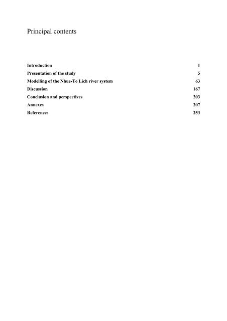
- Page 25 and 26: PART 1: PRESENTATION OF THE STUDY5
- Page 27 and 28: 1. The Nhue-To Lich river basins1.1
- Page 29 and 30: 3.77 m for low and high irrigation,
- Page 31 and 32: 1.2.2. RainfallFigure 1.1.4: Monthl
- Page 33 and 34: Over the whole year, the monthly av
- Page 35 and 36: Figure 1.1.15: Pie chart of land us
- Page 37 and 38: 2. Data base constructionIn order t
- Page 39 and 40: 2.2. Organization of the field surv
- Page 41 and 42: confluence point. The other points
- Page 43 and 44: In summary, the frequency of the ex
- Page 45 and 46: Point Time Level Discharge Cross-se
- Page 47 and 48: conducted independently from the sc
- Page 49 and 50: Figure 1.2.7: DO in on-boat surveyF
- Page 51 and 52: Figure 1.2.9 presents the photos of
- Page 53 and 54: degradable organic fraction in tota
- Page 55 and 56: natural products chemistry led by P
- Page 57 and 58: The analysis of chlorophyll-a is ca
- Page 59 and 60: small comparison between DOC, BOD m
- Page 61 and 62: 3. Hydrology of the Nhue-To Lich ri
- Page 63 and 64: Figure 1.3.3: Gate structure at the
- Page 65 and 66: The rating curve at Cau Den was als
- Page 67 and 68: counted here is constantly distribu
- Page 69 and 70:
4. Water quality of the Nhue-To-Lic
- Page 71 and 72:
Figure 1.4.5: DO extracted from mon
- Page 73 and 74:
the contrary, the low correlation o
- Page 75 and 76:
Figure 1.4.13: PCA of the upstream
- Page 77 and 78:
anthropogenic impact is short at th
- Page 79 and 80:
In conclusion, the seasonal variati
- Page 81 and 82:
NO3 in nitrification process requir
- Page 83 and 84:
PART 2: MODELLING OF THE NHUE-TOLIC
- Page 85 and 86:
IntroductionOne objective of this t
- Page 87 and 88:
definition of the system identifies
- Page 89 and 90:
Y = [(Σ((x c - x m ) 2 /x m,a )/n]
- Page 91 and 92:
3. The validation criteria are form
- Page 93 and 94:
1.2.2. Hydrodynamics and hydraulics
- Page 95 and 96:
AQUASIM's second task is to perform
- Page 97 and 98:
QUAL2 was specifically designed to
- Page 99 and 100:
UK; Wallingford Software 1994); 8 =
- Page 101 and 102:
system will be declared in the next
- Page 103 and 104:
The performance of parameter estima
- Page 105 and 106:
Based on these 3 factors, we have c
- Page 107 and 108:
The lengths of the first, the secon
- Page 109 and 110:
Figure 2.2.2: Rear Thuy Phuong dam
- Page 111 and 112:
2.3.3. Biochemical conceptual schem
- Page 113 and 114:
1973; Yen, 1979; French, 1985). The
- Page 115 and 116:
+ Heterotrophic growth on dissolved
- Page 117 and 118:
The loss of heterotrophic biomass i
- Page 119 and 120:
O 2 /l)P/l)S NH4 : concentration of
- Page 121 and 122:
In contrast, the Nhue river is ofte
- Page 123 and 124:
2.4.2.1.4. Estimation of the kineti
- Page 125 and 126:
In fresh water environment, the equ
- Page 127 and 128:
+ NH 4 exchangeIn this equation, th
- Page 129 and 130:
τ cd : critical shear stress for d
- Page 131 and 132:
The critical shear stress for erosi
- Page 133 and 134:
2.4.2.2.6. Precipitation/dissolutio
- Page 135 and 136:
The table 2.2.9 represents complete
- Page 137 and 138:
3.2. Initial and boundary condition
- Page 139 and 140:
N1TLSpecies Prior simulation After
- Page 141 and 142:
3.3. Simulation prior to calibratio
- Page 143 and 144:
adsorption in our river. The decrea
- Page 145 and 146:
and an intermediate class 2 with
- Page 147 and 148:
3. The half-saturation coefficients
- Page 149 and 150:
negligible factor in the polluted a
- Page 151 and 152:
3.5. Results of the post-calibratio
- Page 153 and 154:
conceptual scheme and in providing
- Page 155 and 156:
case of inundation. We suppose that
- Page 157 and 158:
the inconsistence data employed in
- Page 159 and 160:
4. Simulation of the transient stat
- Page 161 and 162:
water discharge can dilute the diss
- Page 163 and 164:
this modelling period with previous
- Page 165 and 166:
4.4.1.3. Estimation of accumulative
- Page 167 and 168:
4.4.2.2. Boundary conditions for un
- Page 169 and 170:
Figure 2.4.19: Initial condition of
- Page 171 and 172:
The diurnal variation is another tr
- Page 173 and 174:
Figure 2.4.29: Simulated and measur
- Page 175 and 176:
August 1 st to 4 th 2003. Of which
- Page 177 and 178:
The wind speed was predicted from t
- Page 179 and 180:
occurrence is regular whenever rain
- Page 181 and 182:
Figure 2.4.47: Boundary condition o
- Page 183 and 184:
Figure 2.4.55: Simulated and measur
- Page 185 and 186:
Figure 2.4.59: Turbidity at NT1 in
- Page 187 and 188:
PART 3: DISCUSSION167
- Page 189 and 190:
IntroductionIn the previous parts,
- Page 191 and 192:
Figure 3.1.1: Average chlorophyll-a
- Page 193 and 194:
In conclusion, with high nutrient l
- Page 195 and 196:
Dissolved oxygen (g O 2 /m 2 /d) NH
- Page 197 and 198:
- DO balanceFigure 3.1.9: Dissolved
- Page 199 and 200:
- NH 4 balanceFigure 3.1.11: NH 4 b
- Page 201 and 202:
Figure 3.1.14: NH 4 balance in summ
- Page 203 and 204:
Figure 3.1.15: Exponential relation
- Page 205 and 206:
2. Investigations toward restoratio
- Page 207 and 208:
Figure 3.2.3: Simulation based on d
- Page 209 and 210:
The distance of recovery is hardly
- Page 211 and 212:
upstream inflow. It also implies th
- Page 213 and 214:
So far, the wastewater of the Hanoi
- Page 215 and 216:
The simulation results of two varia
- Page 217 and 218:
Figure 3.2.17: DO at NT2 in differe
- Page 219 and 220:
Figure 3.2.21: Evolution of DO at d
- Page 221 and 222:
As shown in simulation results, the
- Page 223 and 224:
Conclusion and perspectivesConclusi
- Page 225 and 226:
processes which were not measured.
- Page 227 and 228:
1. Annex 1: Experimental protocols
- Page 229 and 230:
PO 4P totalRange Method Standardsol
- Page 231 and 232:
- Analytical methods+ BOD: Water sa
- Page 233 and 234:
MgClSO 4HCO 3TraceelementsRange Met
- Page 235 and 236:
2. Annex 2: Estimation of organic m
- Page 237 and 238:
Ratios between heterotrophic bacter
- Page 239 and 240:
- To assess the individual local pa
- Page 241 and 242:
δmabsj=1n∑n i=1sijParameter rank
- Page 243 and 244:
The above definition has a simple i
- Page 245 and 246:
4. Annex 4: Mathematical formulas i
- Page 247 and 248:
⎛∧ ⎜j = ⎜QC⎜⎝iQ ⎞∂C
- Page 249 and 250:
6. Annex 6: Stoichiometric coeffici
- Page 252 and 253:
Subs. ValueUnitaerobic sediment exc
- Page 254 and 255:
kwind⎛= ⎜⎝ 3.6e1−1 225 10
- Page 257 and 258:
DO evolution in Bell Jar experiment
- Page 259 and 260:
Firstly of all, NH 4 and DO behave
- Page 261 and 262:
Results of Bell Jar experiment at T
- Page 263 and 264:
As clearly observed in the figure a
- Page 265 and 266:
10. Annex 10: Parameter estimation
- Page 267 and 268:
and parameter estimation. It is exp
- Page 269 and 270:
First of all, an experimental layou
- Page 271 and 272:
ate of phytoplankton also ranks low
- Page 273 and 274:
ReferencesAalderink R.H., Klaver N.
- Page 275 and 276:
Brown L.C. and Barnwell T.O. (1987)
- Page 277 and 278:
Henze M., Grady C.P.L., Gujer W., M
- Page 279 and 280:
Liss, P.S. and Slater, P.G. (1974)
- Page 281 and 282:
Prieur N. (2001) Dynamique des cont
- Page 283 and 284:
Smith, V. H., Tilman G. D., and Nek
- Page 285:
Zonneveld C. (1998) A cell-based mo