Variable-step preconditioned conjugate gradient method for partial ...

More documents

Recommendations

Info

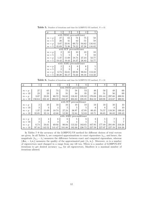
Table 5. Number of iterations and time for LOBPCG-VS method, N = 31 p 1 2 3 4 5 with DIAG preconditioner m = p 27 65 74 75 58 m = 5 26 41 42 51 58 m = p 3.07 23.91 60.72 94.62 116.82 m = 5 45.69 72.36 79.22 97.20 116.82 with ICF preconditioner m = p 2 10 10 10 10 m = 5 5 5 6 7 10 m = p 1.37 11.69 18.74 27.24 52.77 m = 5 19.42 19.43 24.37 26.83 52.77 with AMG preconditioner m = p 2 4 6 6 5 m = 5 2 3 4 4 5 m = p 6.74 24.61 69.92 90.04 113.32 m = 5 40.28 56.17 72.33 88.16 113.32 Table 6. Number of iterations and time for LOBPCG-VS method, N = 31 p 1 2 3 4 5 6 7 8 9 10 with DIAG preconditioner m = p 27 65 74 75 58 53 46 50 49 69 m = 10 23 23 31 31 34 35 35 51 56 69 m = p 3.07 23.91 60.72 94.62 116.82 135.92 170.08 231.44 297.68 490.91 m = 10 150.64 222.42 202.03 233.37 263.83 228.85 264.52 349.98 413.67 490.91 with ICF preconditioner m = p 2 10 10 10 10 10 10 10 10 10 m = 10 3 3 4 5 5 5 6 8 8 10 m = p 1.37 11.69 18.74 27.24 36.97 47.95 60.45 74.57 110.50 109.43 m = 10 32.05 32.14 42.68 52.99 52.84 52.83 63.71 86.65 86.83 109.43 with AMG preconditioner m = p 2 4 6 6 5 6 6 5 7 7 m = 10 2 3 3 4 4 5 5 5 5 7 m = p 6.74 24.61 69.92 90.04 113.32 163.65 167.95 177.49 291.89 316.26 m = 10 97.16 142.52 141.47 181.88 182.30 226.72 227.59 227.07 227.19 316.26 In Tables 7–9 the accuracy of the LOBPCG-VS method for different choices of trial vectors are given. In all Tables λi are computed approximations to exact eigenvalues λh,i, and hence, the magnitude |λh,i − λi| measures the difference between exact and computed eigenvalues, whereas �Avi − λivi� measures the quality of the approximated pair {λi, vi}. Moreover, m is a number of eigenvectors used changed in a range from one till ten, NIters is a number of LOBPCG-EV iterations to get desired accuracy ε0ut for all eigenvectors, MaxIters is a maximal number of iterations allowed. 12
Table 7. Number of iterations for LOBPCG-VS method with DIAG preconditioner, p = m m 1 2 3 4 5 NIters 27 65 74 75 58 |λh,1 − λ1| 0.484 ·10 −5 0.213 ·10 −9 0.355 ·10 −11 0.336 ·10 −5 0.208 ·10 −11 |λh,2 − λ2| - 0.563 ·10 −5 0.153 ·10 −7 0.750 ·10 −10 0.544 ·10 −8 |λh,3 − λ3| - - 0.961 ·10 −5 0.247 ·10 −6 0.103 ·10 −5 |λh,4 − λ4| - - - 0.329 ·10 −5 0.537 ·10 −5 |λh,5 − λ5| - - - - 0.516 ·10 −6 �Av1 − λ1v1� 0.18713 ·10 −2 0.999 ·10 −5 0.155 ·10 −5 0.159 ·10 −2 0.134 ·10 −5 �Av2 − λ2v2� - 0.167 ·10 −2 0.811 ·10 −4 0.679 ·10 −5 0.686 ·10 −4 �Av3 − λ3v3� - - 0.182 ·10 −2 0.397 ·10 −3 0.870 ·10 −3 �Av4 − λ4v4� - - - 0.127 ·10 −2 0.183 ·10 −2 �Av5 − λ5v5� - - - - 0.480 ·10 −3 m 6 7 8 9 10 NIters 53 46 50 49 69 |λh,1 − λ1| 0.288 ·10 −10 0.103 ·10 −9 0.172 ·10 −4 0.222 ·10 −11 0.783 ·10 −17 |λh,2 − λ2| 0.177 ·10 −7 0.161 ·10 −7 0.705 ·10 −10 0.165 ·10 −10 0.568 ·10 −15 |λh,3 − λ3| 0.446 ·10 −6 0.671 ·10 −6 0.556 ·10 −7 0.361 ·10 −8 0.383 ·10 −5 |λh,4 − λ4| 0.525 ·10 −5 0.132 ·10 −5 0.423 ·10 −8 0.410 ·10 −8 0.925 ·10 −14 |λh,5 − λ5| 0.154 ·10 −6 0.390 ·10 −6 0.171 ·10 −4 0.106 ·10 −8 0.208 ·10 −13 |λh,6 − λ6| 0.333 ·10 −5 0.290 ·10 −5 0.382 ·10 −7 0.180 ·10 −7 0.623 ·10 −12 |λh,7 − λ7| - 0.528 ·10 −5 0.715 ·10 −6 0.717 ·10 −7 0.424 ·10 −11 |λh,8 − λ8| - - 0.621 ·10 −5 0.819 ·10 −6 0.353 ·10 −10 |λh,9 − λ9| - - - 0.347 ·10 −4 0.447 ·10 −8 |λh,10 − λ10| - - - - 0.164 ·10 −6 �Av1 − λ1v1� 0.476 ·10 −5 0.904 ·10 −5 0.115 ·10 −2 0.182 ·10 −5 0.272 ·10 −8 �Av2 − λ2v2� 0.115 ·10 −3 0.122 ·10 −3 0.837 ·10 −5 0.391 ·10 −5 0.247 ·10 −7 �Av3 − λ3v3� 0.604 ·10 −3 0.750 ·10 −3 0.206 ·10 −3 0.649 ·10 −4 0.184 ·10 −2 �Av4 − λ4v4� 0.153 ·10 −2 0.102 ·10 −2 0.534 ·10 −4 0.625 ·10 −4 0.958 ·10 −7 �Av5 − λ5v5� 0.238 ·10 −3 0.484 ·10 −3 0.118 ·10 −2 0.332 ·10 −4 0.139 ·10 −6 �Av6 − λ6v6� 0.142 ·10 −2 0.109 ·10 −2 0.156 ·10 −3 0.126 ·10 −3 0.682 ·10 −6 �Av7 − λ7v7� - 0.198 ·10 −2 0.570 ·10 −3 0.214 ·10 −3 0.165 ·10 −5 �Av8 − λ8v8� - - 0.172 ·10 −2 0.755 ·10 −3 0.490 ·10 −5 �Av9 − λ9v9� - - - 0.197 ·10 −2 0.495 ·10 −4 �Av10 − λ10v10� - - - - 0.230 ·10 −3 From the results in Table 7 one can see that the number of iterations is only slightly changed when m is growing. It shows that the theoretical rate of convergence given in Theorem 1 and 2 is not sharp for the block case and give only an upper bound. The accuracy both eigenvalues and eigenvectors is always better when m is growing, but it is improved nonuniformly. Moreover, there are some problems with multiple eigenvalues. Indeed, λ2 = λ3 and one can see that the accuracy for λ3 and v3 is always one or two order of magnitude worse as for λ2 and v2. The present inconsistency between numerical and theoretical results can be explained by the slow convergence behaviour of the variable-step preconditioning method, i.e. we could not reach the desired accuracy εin, and hence, the actual reduction factor q is greater as theoretical one q(εin, λkj , λkj+1) from Theorem 4. 13
Page 1 and 2: Variable-step preconditioned conjug
Page 3 and 4: which is too complicated for unders
Page 5 and 6: Theorem 1 shows that a certain sequ
Page 7 and 8: Algorithm LOBPCG-VS Input: m starti
Page 9 and 10: 6 Numerical results All numerical r
Page 11: Since all results in Table 1 and 2
Page 15 and 16: Table 9. Number of iterations for L
Page 17 and 18: [11] A.V. Knyazev, New estimates fo
Page 19: Appendix B Without loss of generall

Variable-step preconditioned conjugate gradient method for partial ...

Create successful ePaper yourself

Delete template?

Save as template?