Variable-step preconditioned conjugate gradient method for partial ...

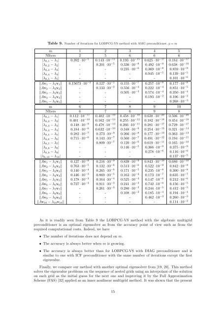
Table 9. Number of iterations for LOBPCG-VS method with AMG preconditioner, p = m
m 1 2 3 4 5
NIters 2 5 6 6 6
|λh,1 − λ1| 0.392 ·10 −5 0.143 ·10 −11 0.193 ·10 −15 0.625 ·10 −17 0.184 ·10 −17
|λh,2 − λ2| - 0.201 ·10 −5 0.336 ·10 −8 0.492 ·10 −9 0.638 ·10 −10
|λh,3 − λ3| - - 0.235 ·10 −6 0.369 ·10 −8 0.859 ·10 −9
|λh,4 − λ4| - - - 0.945 ·10 −5 0.139 ·10 −5
|λh,5 − λ5| - - - - 0.101 ·10 −6
�Av1 − λ1v1� 0.15673 ·10 −2 0.127 ·10 −5 0.155 ·10 −7 0.257 ·10 −8 0.177 ·10 −8
�Av2 − λ2v2� - 0.133 ·10 −2 0.556 ·10 −4 0.222 ·10 −4 0.851 ·10 −5
�Av3 − λ3v3� - - 0.505 ·10 −3 0.574 ·10 −4 0.350 ·10 −4
�Av4 − λ4v4� - - - 0.193 ·10 −2 0.106 ·10 −2
�Av5 − λ5v5� - - - - 0.268 ·10 −3
m 6 7 8 9 10
NIters 6 7 6 9 8
|λh,1 − λ1| 0.112 ·10 −17 0.402 ·10 −19 0.458 ·10 −18 0.638 ·10 −20 0.506 ·10 −20
|λh,2 − λ2| 0.401 ·10 −10 0.162 ·10 −13 0.255 ·10 −12 0.182 ·10 −18 0.454 ·10 −18
|λh,3 − λ3| 0.148 ·10 −9 0.478 ·10 −13 0.266 ·10 −11 0.281 ·10 −17 0.729 ·10 −17
|λh,4 − λ4| 0.184 ·10 −6 0.632 ·10 −10 0.348 ·10 −9 0.254 ·10 −15 0.321 ·10 −14
|λh,5 − λ5| 0.282 ·10 −7 0.273 ·10 −9 0.266 ·10 −8 0.177 ·10 −13 0.363 ·10 −13
|λh,6 − λ6| 0.715 ·10 −6 0.143 ·10 −7 0.560 ·10 −7 0.491 ·10 −12 0.194 ·10 −11
|λh,7 − λ7| - 0.809 ·10 −7 0.120 ·10 −6 0.619 ·10 −11 0.165 ·10 −10
|λh,8 − λ8| - - 0.146 ·10 −5 0.366 ·10 −9 0.375 ·10 −9
|λh,9 − λ9| - - - 0.278 ·10 −6 0.116 ·10 −6
|λh,10 − λ10| - - - - 0.137 ·10 −5
�Av1 − λ1v1� 0.127 ·10 −8 0.216 ·10 −9 0.839 ·10 −9 0.843 ·10 −10 0.680 ·10 −10
�Av2 − λ2v2� 0.763 ·10 −5 0.132 ·10 −6 0.513 ·10 −6 0.522 ·10 −9 0.842 ·10 −9
�Av3 − λ3v3� 0.140 ·10 −4 0.265 ·10 −6 0.171 ·10 −5 0.235 ·10 −8 0.300 ·10 −8
�Av4 − λ4v4� 0.446 ·10 −3 0.869 ·10 −5 0.163 ·10 −4 0.173 ·10 −7 0.635 ·10 −7
�Av5 − λ5v5� 0.178 ·10 −3 0.164 ·10 −4 0.525 ·10 −4 0.147 ·10 −6 0.212 ·10 −6
�Av6 − λ6v6� 0.727 ·10 −3 0.911 ·10 −3 0.241 ·10 −3 0.742 ·10 −6 0.156 ·10 −5
�Av7 − λ7v7� - 0.261 ·10 −3 0.280 ·10 −3 0.244 ·10 −5 0.412 ·10 −5
�Av8 − λ8v8� - - 0.108 ·10 −2 0.185 ·10 −4 0.194 ·10 −4
�Av9 − λ9v9� - - - 0.462 ·10 −3 0.260 ·10 −3
�Av10 − λ10v10� - - - - 0.114 ·10 −2
As it is readily seen from Table 9 the LOBPCG-VS method with the algebraic multigrid
preconditioner is an optimal eigensolver as from the accuracy point of view such as from the
required computational costs. Indeed, we have
• The number of iterations does not depend on m.
• The accuracy is always better when m is growing.
• The accuracy is always better than for LOBPCG-VS with DIAG preconditioner and is
similar to one with ICF preconditioner with the same number of iterations except the first
eigenvalue.
Finally, we compare our method with another optimal eigensolver from [19, 20]. This method
solves the eigenvalue problems on the sequence of nested grids using an interpolant of the solution
on each grid as the initial guess for the next one and improving it by the Full Approximation
Scheme (FAS) [32] applied as an inner nonlinear multigrid method. It was shown that the present
15